A Framework for Short Video Recognition Based on Motion Estimation and Feature Curves on SPD Manifolds

Abstract

Given the prosperity of video media such as TikTok and YouTube, the requirement of short video recognition is becoming more and more urgent. A significant feature of short video is that there are few switches of scenes in short video, and the target (e.g., the face of the key person in the short video) often runs through the short video. This paper presents a new short video recognition algorithm framework that transforms a short video into a family of feature curves on symmetric positive definite (SPD) manifold as the basis of recognition. Thus far, no similar algorithm has been reported. The results of experiments suggest that our method performs better on three changeling databases than seven other related algorithms published in the top issues.

1. Introduction

Video, especially short video, has become the mainstream information medium on the Internet. Facing the huge daily output and segmented production of short videos, however, review and recommendation of short video still highly dependent on tag-based and manual recognition. In order to achieve more intelligent and efficient content audit, short video recognition algorithms are in great demand. Since the first step of recognition is feature extraction, many feature extraction methods based on static image have been established. However, their application to video data still faces great challenges. Meanwhile, Riemannian manifolds have been proven to be robust in extracting video features under different imaging conditions and therefore have been successfully employed in many branches of video recognition, including face recognition and action recognition.

In particular, symmetric positive definite (SPD) matrices are widely used in video representation because of second-order statistical information provided. Moreover, the space of all SPD matrices possessing the Riemannian metric is called SPD manifold [1,2]. In general, existing SPD-based methods for video recognition construct an SPD matrix to represent each video and then take the resulting SPD manifold into account for recognition; for example, modeling video as covariance matrix [3], kernel matrix [4,5], and Gaussian model [6,7].

Moreover, dimensionality reduction (DR) techniques can effectively extract valid information from the original SPD matrix and reduce the calculation cost drastically with regard to the dimension of SPD matrix. One of the DR approaches directly extracts feature vector, which is in the Euclidean space, from the original SPD matrix, taking the notions of Riemannian geometry [8]. Or, to maintain SPD geometry, the bilinear DR [9,10] aims to learn a mapping that transforms the original manifold into a new manifold. This new manifold possesses a lower dimension and a more discriminative metric. Metric learning on SPD manifolds learns a more discriminative function that narrows the similarity between SPD matrices from different categories while expanding the similarity between SPD matrices from the same category. Metric learning on SPD manifold usually projects the original SPD manifolds to their tangent space [11,12], or embeds the SPD manifolds to a subspace of reproducing the kernel Hilbert space (RKHS) [13,14,15]. The tangent space and subspace of RKHS are isomorphic with Euclidean spaces that possess the same dimension.

It is obvious that the SPD-based methods introduced above regard the whole video as an image-set-based SPD matrix but without considering temporal correlation between frame images. Moreover, the experiments of these methods are based on databases composed of segmented video clips. These video clips are actually short videos. Through the benefit of the few transitions in short videos, tracing the trajectories of regions of interest (ROIs) through video is available. Moreover, in order to extract both spatial and temporal features from video, the authors of [16,17] adopted space-time geometric representations of human landmark configurations. Inspired by the work in [16,17], we propose a framework for short video recognition that models the spatiotemporal trajectories of ROIs as a family of feature curves on SPD manifold in this paper. The main steps of our short video recognition framework are as follows:

(1)

According to the practical application, a key frame is extracted from the short video to determine the spatial feature blocks (i.e., ROIs) of the target.

(2)

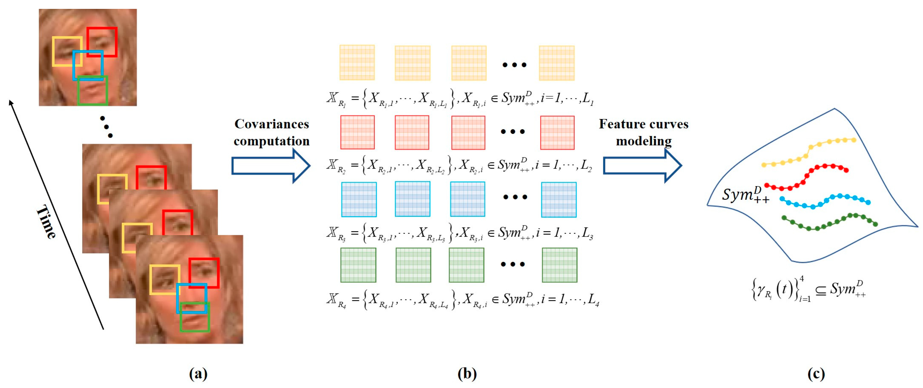
Using motion estimation [18] in video encoding, each ROI in the key frame is traced forward, backward, or two-way to string time series of ROIs through the short video. The resulting family of time series of ROIs represent the temporal and spatial feature of short video.

(3)

Each ROI is transformed into an SPD matrix by regional covariance descriptor (RCD). Hence, the family of time series of ROIs is transformed into a family of time series of SPD matrices. Each obtained time series of SPD matrices is a curve on the SPD manifold. The family of curves is the feature curves of the short video, which is the basis of short video recognition.

(4)

Using the dynamic time warping (DTW) [19] with Riemannian metrics [1,2,20] and divergences [21,22] on the SPD manifold, the similarity measure between curve families on the SPD manifold is established, so as to realize the recognition of short video.

Taking face recognition as an example, the overview of our framework is shown in Figure 1. Thus far, no similar algorithm has been reported. The experiments on three databases show that our framework is superior to seven other related algorithms published in the top issue in recent years. The main contributions of this paper are as follows:

(1)

Proposing a short video recognition framework feasible for different applications, as well as providing optional strategies for stringing time series of ROIs, constructing RCDs, and providing recognition between families of feature curves.

(2)

Different from viewing a video as an image set-based SPD matrix, which ignores the temporal correlation of features across image frames, our framework models each video as a family of feature curves on the SPD manifold, considering both temporal and spatial features of video.

(3)

ROI and motion estimation in video encoding are applied in our framework to reduce computational burden due to redundancy across image frames. Compared with using global frame images, ROIs convey more accurate spatial features. Moreover, tracing ROI with motion estimation can effectively reduce the computation of feature detection.

(4)

Encoding major spatial features by ROI-based covariance descriptors helps to build SPD geometry and provides a discriminant Riemannian metric for recognition.

Figure 1. Overview of the proposed framework. Taking face video as example, the four boxes of red, yellow, blue, and green in (a) show the regions of interest (ROIs) on human face and time series of ROIs stringed through motion estimation. The regional covariance descriptors (RCDs) are computed for each region in (b). Hence, a family of feature curves on symmetric positive definite (SPD) manifold are built in (c).

Figure 1. Overview of the proposed framework. Taking face video as example, the four boxes of red, yellow, blue, and green in (a) show the regions of interest (ROIs) on human face and time series of ROIs stringed through motion estimation. The regional covariance descriptors (RCDs) are computed for each region in (b). Hence, a family of feature curves on symmetric positive definite (SPD) manifold are built in (c).

The programming of this paper is as follows. In Section 2, we present notations and preliminaries. In Section 3, several related works are introduced. Section 4 provides the details of our proposed framework. Section 5 introduces the application of our proposed framework in face recognition from video. Section 6 introduces seven SPD-based video/image set recognition algorithms in recent years as comparison algorithms. Section 7 shows the experimental results on three datasets with seven comparison algorithms. Conclusions are given in Section 8.

2. Preliminaries

In this section, we first provide a notation throughout this paper and then introduce geometry of SPD manifold, including the Riemannian metrics on SPD manifold and divergence of SPD matrices. In addition, we provide an introduction about motion estimation in video compression coding.

2.1. Notation

In this paper, vectors are denoted by lower case letters, e.g., $x$; matrices are represented by upper case letters, e.g., $X$; and the set of matrices are represented by $\mathbb{X}=\left\{X_1,\cdots ,X_N\right\}$. $R^D$ is the Euclidean space. $Sy{m}_{++}^D$ is the SPD manifold, which will be formally defined later. $T_X\left(Sy{m}_{++}^D\right)$ is the tangent space to the SPD manifold at $X\in Sy{m}_{++}^D$. $Gr\left(d,D\right)$ is the Grassmannian manifold, i.e., the set of d-dimensional subspaces of $R^D$. $GL\left(D\right)$ is the general linear group, i.e., the set of all invertible $D\times D$ matrices. $Sy{m}_{+}^D$ is a positive semidefinite cone, i.e., the set of all $D\times D$ positive semidefinite matrices. $\mathscr{H}$ is the reproducing kernel Hilbert space.

2.2. The Geometry of SPD Manifold

The $D\times D$ dimensional matrix $X$ is symmetric and positively definite if $X^T=X$ and the scalar $v^{T}Xv>0$ for any non-zero column vector $v\in R^D$. The space of all $D\times D$ dimensional SPD matrixes is expressed as $Sy{m}_{++}^D$. If $Sy{m}_{++}^D$ is given a Riemannian metric, the space of the SPD matrix becomes a Riemannian manifold. Namely, the SPD manifold is defined as

$$Sy{m}_{++}^D=\left\{X\in R^{D\times D}|X^T=X,v^{T}Xv>0 \mathrm{for} \forall v\in R^D\right\}.$$

(1)

For all $X\in Sy{m}_{++}^D$, its tangent space of symmetric $D\times D$ matrices with logarithm mapping $Lo{g}_X:Sy{m}_{++}^D\to T_X\left(Sy{m}_{++}^D\right)$:

$$T_X\left(Sy{m}_{++}^D\right)=\left\{\Phi |\Phi \in R^{D\times D},{\Phi }^T=\Phi \right\}.$$

(2)

The geometry of SPD manifolds is usually learned through Riemannian metrics $\omega$. The Riemannian metric defines the inner product on tangent space. For any $X\in Sy{m}_{++}^D$ and $\Phi ,\Theta \in T_x\left(Sy{m}_{++}^D\right)$,

$$\omega \left(\Phi ,\Theta \right)={\langle \Phi ,\Theta \rangle }_X.$$

(3)

And the inner product reflects the length of the curve between corresponding points on SPD manifold $Sy{m}_{++}^D$. The curve with the shortest distance is the geodesic between two elements on $Sy{m}_{++}^D$. The length of the geodesic is called the geodesic distance.

The affine invariant Riemannian metric (AIRM) [1] is the most frequently used Riemannian metric. For all $\Phi ,\Theta \in T_x\left(Sy{m}_{++}^D\right)$, the AIRM is defined as

$${\langle \Phi ,\Theta \rangle }_X={\langle X^{-1/2}\Phi X^{-1/2},X^{-1/2}\Theta X^{-1/2}\rangle }_F,$$

(4)

where ${\langle A,B\rangle }_F=tr\left(A{B}^T\right)$ and $X\in Sy{m}_{++}^D$. ${\langle \cdot ,\cdot \rangle }_X$ are an inner product and its smoothing over $Sy{m}_{++}^D$, respectively. The logarithm mapping projecting $X_2\in Sy{m}_{++}^D$ to tangent space $T_{X_1}\left(Sy{m}_{++}^D\right)$ is defined as

$$L{\mathrm{og}}_{X_1}\left(X_2\right)=X_1^{\frac{1}{2}}\log \left(X_1^{-\frac{1}{2}}{X}_2^{}{X}_1^{-\frac{1}{2}}\right)X_1^{\frac{1}{2}}.$$

(5)

For any given pair $X_1,X_2\in Sy{m}_{++}^D$, the unique geodesic [23] induced from AIRM connecting ${\Gamma }_{X_1}^{X_2}\left(0\right)=X_1$ with ${\Gamma }_{X_1}^{X_2}\left(1\right)=X_2$ is given by

$${\Gamma }_{X_1}^{X_2}\left(t\right)=X_1^{\frac{1}{2}}\mathit{exp}\left(t \mathit{log}{X}_1^{-\frac{1}{2}}{X}_2^{}{X}_1^{-\frac{1}{2}}\right)X_1^{\frac{1}{2}},t>0.$$

(6)

The geodesic distance between $X_1,X_2\in Sy{m}_{++}^D$ induced from AIRM is as follows:

$${\delta }_{AIRM}^2\left(X_1,X_2\right)={\Vert \mathit{log}\left(X_1^{-1/2}{X}_2{X}_1^{-1/2}\right)\Vert }_F^2,$$

(7)

where ${\Vert A\Vert }_F^2={\langle A,A\rangle }_F$ is the Frobenius norm of a matrix. The AIRM possesses a property of invariance to affine transformations, i.e., ${\delta }_{AIRM}^2\left(X_1,X_2\right)={\delta }_{AIRM}^2\left(A{X}_1{A}^T,A{X}_2{A}^T\right)$ for $\forall A\in GL\left(D\right)$.

For all $\Phi ,\Theta \in T_x\left(Sy{m}_{++}^D\right)$, the log-Euclidean metric (LEM) [2,20] is defined as

$${\langle \Phi ,\Theta \rangle }_X=\langle D_X\mathit{log}\left(\Phi \right),D_X\mathit{log}\left(\Theta \right)\rangle ,$$

(8)

where $X\in Sy{m}_{++}^D$ and $D_X\mathit{log}\left(\Phi \right)$ denote the directional derivative of $\mathit{log}\left(\Theta \right)$ at $X$. The logarithm mapping projecting $X_2\in Sy{m}_{++}^D$ to tangent space $T_{X_1}\left(Sy{m}_{++}^D\right)$ is defined as

$$Lo{g}_{X_1}\left(X_2\right)=D^{-1}\mathit{log}\left(X_1\right)\left[\mathit{log}\left(X_2\right)-\mathit{log}\left(X_1\right)\right].$$

(9)

Hence, the distance between $X_1,X_2\in Sy{m}_{++}^D$ induced from LEM is as follows:

$${\delta }_{LEM}^2\left(X_1,X_2\right)={\Vert \mathit{log}\left(X_1\right)-\mathit{log}\left(X_2\right)\Vert }_F^2.$$

(10)

2.3. Bregman Divergences

In addition to the distance generated by the Riemannian metric, the divergence of the SPD matrix based on Bregman divergence can also be used as the distance metric of the SPD matrix. For all $X_1,X_2\in Sy{m}_{++}^D$, the Bregman matrix divergence [24] is defined as

$${\delta }_{\varphi }\left(X_1,X_2\right)=\varphi \left(X_1\right)-\varphi \left(X_2\right)-{\langle {\nabla }_{\varphi \left(X_2\right)},X_1-X_2\rangle }_F,$$

(11)

where $\varphi :Sy{m}_{++}^D\to R$ is a strictly convex function, and ${\nabla }_{\varphi \left(X_2\right)}$ is the gradient of $\varphi$ at point $X_2$. Bregman divergence is similar to distance measure, which does not satisfy trigonometric inequality and symmetry. To symmetrize Bregman divergences, different seed functions $\varphi$ are used. Among them, the Stein divergence [21] and Jeffrey divergence [22] play an important role in computer vision.

For any given pair $X_1,X_2\in Sy{m}_{++}^D$, the Stein divergence adopting $\varphi \left(X\right)=-\mathit{log}\mathit{det}\left(X\right)$ and Jensen–Shannon symmetrization is defined as

$${\delta }_S^2\left(X_1,X_2\right)=\mathit{log}\mathit{det}\left(\frac{X_1+X_2}{2}\right)-\frac{1}{2}\mathit{log}\mathit{det}\left(X_1{X}_2\right).$$

(12)

For any given pair $X_1,X_2\in Sy{m}_{++}^D$, the Jeffrey divergence adopting $\varphi \left(X\right)=-\mathit{log}\mathit{det}\left(X\right)$ and direct symmetrization is defined as

$${\delta }_J^2\left(X_1,X_2\right)=\frac{1}{2}tr\left(X_1^{-1}{X}_2\right)+\frac{1}{2}tr\left(X_2^{-1}{X}_1\right)-D,$$

(13)

where $D$ is the dimension of manifold. In the same way as the AIRM, the Stein divergence and Jeffrey divergence are affine invariant.

2.4. Motion Estimation

The similarity between adjacent frames brings inter-frame redundancy. Using motion estimation [18], only the changing parts of adjacent video frames would be encoded to reduce the amount of data and reduce the inter frame redundancy. In motion estimation, a frame image is segmented into $M\times N$ or more commonly used $N\times N$ pixel block. At the matching window of $\left(N+2p\right)\times \left(M+2p\right)$ size, the current block is compared with the corresponding block in the previous frame. This ‘$p$’ referring to pixels adjacent to the ROI is called the search parameter. On the basis of the matching criteria, the best match is found, and the alternative position of the current block is obtained.

There are various matching criteria, including the mean absolute difference (MAD):

$$MAD=\frac{1}{MN}{\displaystyle \sum _{i=1}^M{\displaystyle \sum _{j=1}^N\left|f_k\left(i,j\right)-f_{k-1}\left(i,j\right)\right|}},$$

(14)

mean squared error (MSE):

$$MSE=\frac{1}{MN}{{\displaystyle \sum _{i=1}^M{\displaystyle \sum _{j=1}^N\left[f_k\left(i,j\right)-f_{k-1}\left(i,j\right)\right]}}}^2,$$

(15)

and normalized cross correlation (NCC):

$$NCC=\frac{\frac{1}{MN}{\displaystyle \sum _{i=1}^M{\displaystyle \sum _{j=1}^N\left(f_k\left(i,j\right)-\overline{f_k\left(i,j\right)}\right)\left(f_{k-1}\left(i,j\right)-\overline{f_{k-1}\left(i,j\right)}\right)}}}{\sqrt{\frac{1}{MN}{\displaystyle \sum _{i=1}^M{\displaystyle \sum _{j=1}^N{\left(f_k\left(i,j\right)-\overline{f_k\left(i,j\right)}\right)}^2}}}\sqrt{\frac{1}{MN}{\displaystyle \sum _{i=1}^M{\displaystyle \sum _{j=1}^N{\left(f_{k-1}\left(i,j\right)-\overline{f_{k-1}\left(i,j\right)}\right)}^2}}}},$$

(16)

where $f_k\left(i,j\right)$ are the pixels in the current $M\times N$ block and $f_{k-1}\left(i,j\right)$ are the pixels in the matching block in the frame $k-1$. When MSE or MAD is the smallest, it means that the matching between the two blocks is the best. The difference is that NCC measures the similarity between the two blocks in the range of $\left[-1,1\right]$. The closer the NCC is to 1, the closer the two blocks are to have a linear relationship.

3. Related Works

In this section, we introduce relevant literature that have modeled the temporal evolution of video as curves on the Riemannian manifold. In addition, we also introduce classification and alignment methods of time series.

3.1. Modeling of Video as Curve on Riemannian Manifold

The key point here is to account for the temporal features and spatial features of video simultaneously. Profiting from explicit landmark configurations, several recent works modeled each sequence of facial expressions in video as a curve or a trajectory on Riemannian manifolds. Taheri et al. [25] represented a sequence of faces as a sequence of facial landmarks. Since landmark configuration on each face is a full rank $D\times d$ matrix encoding $d$ dimensional coordinates of $D$ landmarks, a sequence of facial expression can be considered as a curve on the Grassmannian manifold $Gr\left(d,D\right)$ with the neutral face as the starting point. To classify the curves modeled, the linear discriminant analysis (LDA) and multi-class SVM are applied. Taking texture information into consideration, Otberdout et al. [16] encoded deep convolutional neural network features extracted from human faces by covariance descriptors so as to model the temporal revolution of facial expression as trajectory on SPD manifolds.

Besides its role in the field of facial expression recognition, temporal modeling based on landmarks on Riemannian manifolds can extend to action recognition [17,26,27,28,29]. Kacem et al. [17] represents each $D\times d$ landmark matrix of skeleton by a $D\times D$ positive semidefinite Gram matrix. By doing so, the temporal evolution of skeletons is represented by a time series of their corresponding Gram matrices, which can be considered as a trajectory connected by pseudo-geodesics [23] on positive semidefinite cone $Sy{m}_{+}^D$. Devanne et al. [26] used square-root velocity function to construct trajectories in a n-dimensional space representing skeleton sequences. Tanfous et al. [27] represented the landmark configuration sequence as the trajectory in Kendall shape space and encoded the trajectory through the dictionary learned in the sample set to generate Euclidean sparse time series.

However, all these works rely on geometric information from landmarks. These methods not only consume too much to detect landmarks in each frame, but also are not friendly to video without clear landmarks. Moreover, features extracted from pixel-level landmarks are limited. Distinct from works introduced above, in this paper, we focused on modeling curves of ROIs. By determining the pattern of ROIs, different applications of video recognition can be realized, but not only facial expression recognition and action recognition.

3.2. Dynamic Time Warping

The classification methods of time series can be roughly divided into four categories, namely, deep learning (e.g., fully convolutional networks [30]), feature learning method (e.g., time series forest [31]), ensemble methods (e.g., elastic ensemble [32]), and distance learning methods [19,33,34,35,36] with dynamic time warping (DTW) as a development basis.

DTW [19] was originally used in the field of speech recognition, elongating or shortening (compresses) the unknown speech until it is consistent with the length of the reference template. In this process, the time axis of the unknown speech will be distorted or bent so that it can correspond to the standard pattern. This is given two time series $T_1=\left\{a_1,\cdots ,a_{L_1}\right\}$ and $T_2=\left\{b_1,\cdots ,b_{L_2}\right\}$ with lengths of $L_1$ and $L_2$, respectively. A pair of warping paths $\beta =\left({\beta }_1,{\beta }_2\right)$ between $T_1$ and $T_2$ need to meet the following constraints:

$$1={\beta }_1\left(1\right)\le \cdots \le {\beta }_1\left(q\right)=L_1,$$

(17)

$$1={\beta }_2\left(1\right)\le \cdots \le {\beta }_2\left(q\right)=L_2,$$

(18)

$$q\le \mathit{max}\left(L_1,L_2\right)\le L_1+L_2-1.$$

(19)

The optimal path between $T_1$ and $T_2$ is given by

$${\beta }^{*}=\mathit{arg} \underset{\beta \in \Gamma }{\mathit{min}}{\displaystyle \sum _{i=1}^{\left|\beta \right|}\delta \left(T_1{}_{{\beta }_1\left(i\right)},T_{2{\beta }_2\left(i\right)}\right)} ,$$

(20)

where $\Gamma$ is the set of all possible paths and $\delta \left(\cdot ,\cdot \right)$ is a distance metric. The DTW distance is given by

$${\delta }_{DTW}\left(T_1,T_2\right)={\displaystyle \sum _{i=1}^{\left|\beta *\right|}\delta \left(T_1{}_{{\beta }_1^{*}\left(i\right)},T_2{}_{{\beta }_2^{*}\left(i\right)}\right)}.$$

(21)

To sum up, searching for an optimal DTW path ${\beta }^{*}$ is equivalent to finding the optimal solution from all possible warping paths according to minimizing the cumulative distance cost. The recurrence of cumulative distance matrix $\Pi$ with $\Pi \left(0,0\right)=0$ in DTW can be written as

$$\Pi \left(i,j\right)=\delta (a_i,b_j)+\mathit{min}\left\{\Pi \left(i-1,j-1\right),\Pi \left(i-1,j\right),\Pi \left(i,j-1\right)\right\}.$$

(22)

Developed from DTW, the 1NN-DTW model [19,33], which is the combination of 1NN classifier and DTW, variant DDDTW [34], which is based on derivative distance, and constructing kernel function using DTW distance [35,36] are widely used in time series classification. Utilizing DTW distance instead of Euclidean distance for calculating Gaussian RBF kernel, Bahlmann et al. proposed the Gaussian DTW (GDTW) kernel [35]. However, since DTW distance is not symmetric, the GDTW kernel is also not a symmetric kernel. To overcome this limitation, global alignment kernels (GAK) [36] used in [16] need to calculate all the alignments, despite the huge computational cost.

4. A Framework for Feature Curves on SPD Manifold

In this section, we provide the formulation of short video recognition firstly, then present our framework, which represents short video as a family of feature curves on the SPD manifold. Specifically, our framework involves three parts: stringing time series of ROIs based on motion estimation, feature curve modeling with RCDs, and the classification methods of feature curves.

4.1. Formulation of Short Video Recognition

Video recognition is to identify the corresponding label of a query video $V_{query}$ based on a number of sample videos $\left\{V_1,\cdots ,V_n\right\}$ labeled with $\left\{l_1^V,\cdots ,l_n^V\right\}$, which covers face recognition, scene classification, action recognition, and other different application directions. For example, the recognition of surveillance video in the field of the public is to match a query video $V_{query}$ against the video library obtained by the monitoring system. The target to be recognized in the video can be the person, car, or even license plate involved in the case.

This paper focuses on short video recognition. Short videos are now popular in social media with their high-frequency output and strong participation. Hence, video media have high requirements for content audit, information screening, and content recommendation. It is necessary to promote the research of short video recognition. To extract features for recognition, static images are normally described in terms of feature vectors, and videos are regarded as image sets. However, image set ignores the temporal feature of video. Spatial features in video dynamically change in the time dimension, and adjacent frames share similar spatial features. Different from long video, such as movies, the transition or conversion in short video between paragraphs and scenes are minor, which means the significant spatial features, i.e., ROI, may run through the whole short video. To extract spatial-temporal features from short videos, we proposed a framework focusing on the short video recognition model spatiotemporal trajectory of ROI in video as a family of feature curves on the SPD manifold.

4.2. Stringing Time Series of ROIs Based on Motion Estimation

Given a k-frames video $\mathbb{F}=\left\{F_1,\cdots ,F_k\right\}$, where $F_i$ is the image matrix, the spatial features of video are reflected within the frame image of a video. Our proposed framework takes the ROIs of the frame image as the major spatial feature of video. ROI is originally a concept in video encoding. In video encoding, the image quality of non-concerned regions can be sacrificed, and only high-resolution coding can be carried out for key regions, i.e., ROI, to meet the requirements of users’ high-definition video monitoring, while saving network bandwidth, processing time, and video storage space. ROI can be square, round, irregular shape, and so on. In our framework, we first extract a key frame from video, then determine a group of ROIs as a pattern. The ROI possesses semantic features and varies according to specific applications. As an algorithm framework, the solution of ROI selection and ROI detection are open. Meanwhile, the weight and number of ROIs can be adjusted to optimize the algorithm.

The temporal features of video are reflected in the temporal correlation between video frames. Given a pattern of $m$ ROIs ${\left\{RO{I}_i\right\}}_{i=1}^m$, our proposed framework takes the $m$ corresponding time series of ROIs as the spatiotemporal feature of video. Moreover, we use the motion estimation method in video compression coding to trace ROIs. Tracing can be forward, backward, or bidirectional, depending on the position of key frames in the frame sequence. Taking backward tracing as an example, we introduced a specific strategy for stringing time series of ROIs in the following, including the continuous frame extraction strategy and inter-frame extraction strategy.

Let $RO{I}_{i,1}$ represent the i-th ROI in the key frame $F_s\left(1\le s\le k\right)$. For the continuous frame extraction strategy, we take $F_s$ as starting frame for motion estimation and trace the region closest to $RO{I}_{i,1}$ in the next frame $F_{s+1}\left(s\le s+1\le k\right)$ as $RO{I}_{i,2}$. The difference between regions can be calculated by Equations (14)–(16). Then, frame $F_{s+1}$ becomes the new starting frame for next motion estimation, and so on. Each ROI traced is preserved in a time series of ROIs.

However, the ROIs between adjacent frames may be too similar in some smoothly changing videos and preserving ROIs per frame will cause data redundancy. To tackle this problem, we employed an inter-frame extraction strategy. This strategy still traces ROIs per frame, but if the differences between the traced ROI and $RO{I}_{i,1}$ in $F_s$ is below a certain lower limit $\tau$, the traced ROI is not preserved and the starting frame is kept at $F_s$. Only when the differences between the traced ROI in $F_{s+\eta }$ and $RO{I}_{i,1}$ exceed $\tau$ can the traced ROI be strung into the time series as $RO{I}_{i,2}$; then, the starting frame is replaced by $F_{s+\eta }$ for next motion estimation.

Since both strategies will face the distortion of the prediction result due to the accumulation of error caused by each estimation, our proposed framework stops motion estimation in the ending frame $F_e$ where the error accumulates to an upper limit $\mu$. Thus far, we call it a cycle of motion estimation. After a cycle, we go back to the space domain to detect the ROIs in $\left\{F_{e+1},\cdots ,F_k\right\}$ and redefine the starting frame to repeat a new cycle of motion estimation. By looping the cycle until the end of the video to find all the i-th ROIs on the video timeline, we can construct a time series of the i-th ROIs $ℝ\mathbb{O}{\mathbb{I}}_i=\left\{RO{I}_{i,1},\cdots ,RO{I}_{{i,L}_i}\right\}\left(1\le i\le m\right)$, where $L_i$ is the length of the i-th time series. Therefore, the whole video can be represented by a family of time series of ROIs ${\left\{ℝ\mathbb{O}{\mathbb{I}}_i\right\}}_{i=1}^m={\left\{RO{I}_{i,1},\cdots ,RO{I}_{{i,L}_i}\right\}}_{i=1}^m$, where $m$ represents the number of ROIs in the pattern.

It should be noted that the length $L_i$, upper limits $\mu$, lower limit $\tau$, starting frame $F_s$ and ending frame $F_e$ of each time series can be different. Moreover, the most important factor is by stringing time series of ROIs, our proposed framework combines spatial-temporal features of short videos and transforms task of short video recognition to the recognition between families of time series of ROIs.

4.3. Features Curves on SPD Manifold

Although ROI is a semantic feature region in a frame image, such a feature region is directly composed of image pixels. From the perspective of image recognition, such features are original and rough. Our proposed framework uses a regional covariance descriptor to extract the SPD feature matrix from ROI, so as to transform a family of time series of ROIs into a family of feature curves on the Riemannian manifold. The specific methods are as follows:

For a square ROI $ROI=\left[r_1,r_2,\cdots ,r_d\right]\in R^{D\times d}$, we can simply compute the corresponding RCD by

$$C=\frac{1}{d}{\displaystyle \sum _{i=1}^d\left(r_i-\mu \right)}{\left(r_i-\mu \right)}^T,$$

(23)

where $C\in R^{D\times D}$, $\mu =\frac{1}{d}{\displaystyle \sum _{i=1}^d{r}_i}$.

When the ROI is no longer square, or the size is not uniform and the shape is irregular, we use each pixel of the ROI to generate a feature vector to calculate the covariance matrix. For a ROI with $\lambda$ pixels, each pixel generates a D-dimensional vector. The ROI can be represented as $\left\{v_1,\cdots ,v_{\lambda }\right\}\in R^{D\times \lambda }$, and the corresponding RCD is given by

$$C=\frac{1}{\lambda }{\displaystyle \sum _{i=1}^{\lambda }\left(v_i-{\mu }_v\right)}{\left(v_i-{\mu }_v\right)}^T,$$

(24)

where $C\in R^{D\times D}$, ${\mu }_v=\frac{1}{\lambda }{\displaystyle \sum _{i=1}^{\lambda }{v}_i}$. The method of generating feature vectors is open and can vary with different applications. For example, each pixel can generate a nine-dimensional feature vector, which is composed of RGB values and the first order gradients of RGB values in X and Y directions, respectively. By doing so, no matter how different the shape and size of ROI are, the size of the SPD feature matrix generated by RCD is certainly $9\times 9$. In this way, all the resulting curves are on the SPD manifold shared the same dimension, avoiding the influence of sizes of original ROIs.

Following [3], to avoid the singularity, we adjusted the original RCD as $C\ast =C+\xi I$, where $I$ is an identity matrix and $\xi$ is ${10}^{-3}\times tr\left(C\right)$. Then, we followed the information geometry theory [37] to transform the Gaussian model $\mathcal{N}\left(\mu ,C*\right)$ into a $\left(D+1\right)\times \left(D+1\right)$ dimensional SPD matrix as the final RCD:

$$\mathcal{N}\left(\mu ,C*\right)\sim X=\left[\begin{array}{cc}C*+\mu {\mu }^T& \mu \\ {\mu }^T& 1\end{array}\right],$$

(25)

which means the space of $D$-dimensional Gaussian models has been embedded into the SPD manifold $Sy{m}_{++}^{D+1}$. By doing so, one $RO{I}_{i,j}$ becomes an SPD matrix $X_{i,j}$, and a family of time series of ROIs ${\left\{ℝ\mathbb{O}{\mathbb{I}}_i\right\}}_{i=1}^m={\left\{RO{I}_{i,1},\cdots ,RO{I}_{{i,L}_i}\right\}}_{i=1}^m$ are transformed as a family of time series of their embedding SPD matrices ${\left\{{\mathbb{X}}_{R_i}\right\}}_{i=1}^m={\left\{X_{R_i,1},\cdots ,X_{R_i{,L}_i}|X_{i,j}\in {\mathit{Sym}}_{++}^{D+1}\right\}}_{i=1}^m$.

Consider that the geometry of RCD generated from ROI is a point on SPD manifold. A time series of SPD matrices $\mathbb{X}=\left\{X_1,\cdots ,X_N\right\}$ can be defined as a feature curve ${\gamma \left(t\right)}_{0\le t\le N-1}$ on the SPD manifold that passes through all SPD matrices belonging to $\mathbb{X}$ in sequence from $\gamma \left(0\right)=X_1$ to $\gamma \left(N-1\right)=X_N$. Among them, two adjacent SPD matrices are connected by geodesics:

$$C_{\gamma \left(t\right)\to \gamma (t+1)}\leftarrow {\Gamma }_{X_{t+1}}^{X_{t+2}}, t=0,\cdots ,N-2,$$

(26)

where ${\Gamma }_{X_{t+1}}^{X_{t+2}}\left(T\right)=X_{t+1}^{\frac{1}{2}}\mathit{exp}\left(T \mathit{log}{X}_{t+1}^{-\frac{1}{2}}{X}_{t+2}^{}{X}_{t+1}^{-\frac{1}{2}}\right)X_{t+1}^{\frac{1}{2}},0<T\le 1$. In other words, the feature curve representing a time series of ROIs is spliced by multiple geodesics one by one.

Using this strategy, each time series of ROI can be modeled as a curve on the SPD manifold:

$$ℝ\mathbb{O}{\mathbb{I}}_i=\left\{RO{I}_{i,1},\cdots ,RO{I}_{{i,L}_i}\right\}\Rightarrow {\mathbb{X}}_{R_i}=\left\{X_{R_i,1},\cdots ,X_{R_i{,L}_i}\right\}\Rightarrow {\gamma }_{R_i}\left(t\right).$$

(27)

Thus, a short video can be modeled as a family of curves on the SPD manifold:

$${\left\{ℝ\mathbb{O}{\mathbb{I}}_i\right\}}_{i=1}^m={\left\{RO{I}_{i,1},\cdots ,RO{I}_{{i,L}_i}\right\}}_{i=1}^m\Rightarrow {\left\{{\mathbb{X}}_{R_i}\right\}}_{i=1}^m={\left\{X_{R_i,1},\cdots ,X_{R_i{,L}_i}\right\}}_{i=1}^m\Rightarrow {\left\{{\gamma }_{R_i}\right\}}_{i=1}^m,$$

(28)

where the SPD manifold is proven to be a Riemannian manifold and this family of curves is the family of spatial-temporal feature curves of the video. Algorithm 1 summarizes the steps of computing the family of feature curves.

Algorithm 1 Computing a Family of Feature Curves ${\left\{{\gamma }_{R_i}\left(t\right)\right\}}_{i=1}^m$ on ${\mathit{Sym}}_{++}^{D+1}$

Input: A family of time series of ROIs ${\left\{ℝ\mathbb{O}{\mathbb{I}}_i\right\}}_{i=1}^m={\left\{RO{I}_{i,1},\cdots ,RO{I}_{{i,L}_i}\right\}}_{i=1}^m$ from video Output: A family of feature Curves ${\left\{{\gamma }_{R_i}\left(t\right)\right\}}_{i=1}^m$ /* Compute the SPD matrices of ROIs */ for $i\leftarrow 1$ to $m$    for $j\leftarrow 1{ \mathrm{to} L}_i$ do      $X_{R_i,j}\leftarrow \left[\begin{array}{cc}{C}_{{}_{i,j}}^{*}+{\mu }_{i,j}{\mu }_{i,j}^T& {\mu }_{i,j}\\ {\mu }_{i,j}{\mu }_{i,j}^T& 1\end{array}\right]$    end    /* Compute the geodesic between SPD matrices */    ${\gamma }_{R_i}\left(0\right)\leftarrow X_{R_i,1}$    for $t\leftarrow 0{ \mathrm{to} L}_i-2$ do      $C_{\gamma \left(t\right)\to \gamma (t+1)}\leftarrow {\Gamma }_{X_{t+1}}^{X_{t+2}}$ as Equation (26)    end  end Return A Family of feature Curves ${\left\{{\gamma }_{R_i}\left(t\right)\right\}}_{i=1}^m$

4.4. Rcognition between Famlies of Features Curves

In our proposed method, time series of ROIs are extracted from short video. The comparison of similarity between short videos is transformed into the comparison between families of time series. The length of two time series may not be equal. Moreover, different frame rate, variable durations, and arbitrary starting/ending intensities of video also bring about obstacles. To tackle this problem, we adopted dynamic time warping (DTW) to find an alignment between the two videos.

DTW needs to define appropriate metrics for recognition. As we introduced in Section 4.3, the time series of ROIs are transformed as feature curves in SPD manifolds, which introduces discriminative Riemannian metrics and divergence. Given two feature curves ${\gamma }_1\left(t\right)$ and ${\gamma }_2\left(t\right)$ concatenated by $L_1$ and $L_2$ SPD matrices, respectively, and a pair of warping paths $\beta =\left({\beta }_1,{\beta }_2\right)$ between ${\gamma }_1\left(t\right)$ and ${\gamma }_2\left(t\right)$, similar to the optimal path between time series introduced in Section 3.2, the optimal path in the set of all possible paths $\Gamma$ between two feature curves ${\gamma }_1\left(t\right)$ and ${\gamma }_2\left(t\right)$ is

$${\beta }^{*}=\mathit{arg} \underset{\beta \in \Gamma }{\mathit{min}}{\displaystyle \sum _{i=1}^q\delta \left({\gamma }_1\left({\beta }_1\left(i\right)\right),{\gamma }_2\left({\beta }_2\left(i\right)\right)\right)} ,$$

(29)

where $\delta \left(\cdot ,\cdot \right)$ can be defined as Riemannian metrics/divergence in SPD manifold. Similarity measure between two feature curves ${\gamma }_1\left(t\right)$ and ${\gamma }_2\left(t\right)$ under the optimal path can be defines as

$${\delta }_{DTW}\left({\gamma }_1,{\gamma }_2\right)=\frac{1}{q}{\displaystyle \sum _{i=1}^q\delta \left({\gamma }_1\left({\beta }_1^{\ast }\left(i\right)\right),{\gamma }_2\left({\beta }_2^{\ast }\left(i\right)\right)\right)} .$$

(30)

Then, the similarity measure between two video needs to fuse information provided by each curve of its curve family. The classification strategy can also be divided into two types. One is an overall classification strategy that is suitable for situations where the number of ROIs $m$ in a pattern is smaller. Given a family of feature curves ${\left\{{\gamma }_{R_i}^{query}\left(t\right)\right\}}_{i=1}^m$ extracted from query video $V_{query}$ and sample families of feature curves ${\left\{{\left\{{\gamma }_{R_i}^j\left(t\right)\right\}}_{i=1}^m\right\}}_{j=1}^n$ from sample videos $\left\{V_1,\cdots ,V_n\right\}$, the i-th feature curve ${\gamma }_{R_i}^{query}\left(t\right)\left(1\le i\le m\right)$ in $V_{query}$ is independently compared with all the i-th feature curves ${\left\{\left\{{\gamma }_{R_i}^j\left(t\right)\right\}\right\}}_{j=1}^n\left(1\le i\le m\right)$ in sample videos. This approach extends to each feature curve of $V_{query}$ to obtain the $m\times n$ similarity measure matrix $\Psi$ using DTW distance. The average similarity measure $\frac{1}{m}{\displaystyle \sum _{i=1}^m{\Psi }_{i,j}}\left(1\le j\le n\right)$ of all feature curves from $V_{query}$ represents the similarity measure between query video and sample videos. Taking the KNN classifier as an example, the steps of overall classification method are shown in Algorithm 2.

Algorithm 2 Classification of a Family of Feature Curves ${\left\{{\left\{{\gamma }_{R_i}^j\left(t\right)\right\}}_{i=1}^m\right\}}_{j=1}^n$ on SPD Manifold with Overall Classification Strategy.

Input: $n$ sample families of feature curves ${\left\{{\left\{{\gamma }_{R_i}^j\left(t\right)\right\}}_{i=1}^m,l_j^V\right\}}_{j=1}^n$ with their corresponding labels of each family, a family of feature curves ${\left\{{\gamma }_{R_i}^{query}\left(t\right)\right\}}_{i=1}^m$ of query video $V_{query}$. Output: Predicted label $l_{}^{query}$ of $V_{query}$ /* Compute DTW distances among sample and query feature curves */   for $i\leftarrow 1$ to $m$    for $j\leftarrow 1$ to $n$ do      $\Psi \left(i,j\right)={\delta }_{DTW}\left({\gamma }_{R_i}^{query}\left(t\right),{\gamma }_{R_i}^j\left(t\right)\right)$     end   end /* Compute average DTW distance matrix $\psi$*/   for $k\leftarrow 1$ to $m$ do    $\psi \left(1,k\right)=\frac{1}{m}{\displaystyle \sum _{i=1}^m{\Psi }_{i,k}}$  end /* Testing phase */  $l_{}^{query}\leftarrow$ KNN classifier using average DTW distance matrix $\psi$ Return Predicted label $l_{}^{query}$ of $V_{query}$

The other is the pre-classification strategy suitable for the number of ROIs $m$ in the pattern being larger. Each feature curve of query video $V_{query}$ is pre-classified independently according to each row of similarity measure matrix $\Psi$. On the basis of the law of large numbers [38], the label with the highest frequency among $\left\{l_1^{query},\cdots ,l_m^{query}\right\}$ is regarded as the label of the query video $V_{query}$. Taking the KNN classifier as an example, the steps of the pre-classification method are shown in Algorithm 3.

Algorithm 3 Classification of a Family of Feature Curves ${\left\{{\left\{{\gamma }_{R_i}^j\left(t\right)\right\}}_{i=1}^m\right\}}_{j=1}^n$ on SPD Manifold with Pre-classification Strategy

Input: $n$ sample families of feature curves ${\left\{{\left\{{\gamma }_{R_i}^j\left(t\right)\right\}}_{i=1}^m,l_j^V\right\}}_{j=1}^n$ with their corresponding labels of each family, a family of feature curves ${\left\{{\gamma }_{R_i}^{query}\left(t\right)\right\}}_{i=1}^m$ of query video $V_{query}$. Output: Predicted label $l_{}^{query}$ of query video $V_{query}$ /* Compute distances among sample and query feature curves */  for $i\leftarrow 1$ to $m$    for $j\leftarrow 1$ to $n$ do      $\Psi \left(i,j\right)={\delta }_{DTW}\left({\gamma }_{R_i}^{query}\left(t\right),{\gamma }_{R_i}^j\left(t\right)\right)$     end   end /* Testing phase */   for $k\leftarrow 1$ to $m$ do     $l_k^{query}\leftarrow$ KNN classifier using the k-th row of distance matrix $\Psi$   end   Return Mode of $\left\{l_1^{query},\cdots ,l_m^{query}\right\}$ as predicted label $l_{}^{query}$ of $V_{query}$

In summary, our proposed framework focuses on short video recognition. The few transitions of short videos help to trace the coherent trajectory of ROI with motion estimation. Moreover, stringing time series of ROIs extracts both spatial and temporal features from short video. Furthermore, modeling time series of ROIs as feature curves on the SPD manifold via RCDs introduces the Riemannian geometry. Finally, our framework provides different strategies for stringing time series of ROIs, constructing RCDs, and classifying between families of curves, improving the universality and stability of our framework.

5. Application to Face Recognition

For face recognition in short video, where video $\mathbb{F}=\left\{F_1,\cdots ,F_k\right\}$ can be considered as a sequence of face images, we take the first frame with clear facial features as the key frame and define four square ROIs ${\left\{RO{I}_i\right\}}_{i=1}^4$ located in the four regions around the two eyes, nose, and mouth as a pattern (see Figure 1a). Using the continuous frame extraction strategy to trace ROI backward, we can string four time series of ROIs ${\left\{ℝ\mathbb{O}{\mathbb{I}}_i\right\}}_{i=1}^4$, where $ℝ\mathbb{O}{\mathbb{I}}_i=\left\{RO{I}_{i,1},\cdots ,RO{I}_{i,r_i}\right\}\left(1\le i\le 4\right)$, with embedding SPD matrices ${\left\{{\mathbb{X}}_{R_i}\right\}}_{i=1}^4$ employing Equations (23) and (25). At the same time, in order to combine the global spatial features, we also take the global face $G_1$ in the key frame as the starting point, and link the next two nearest face images in time. For the time series of global spatial features $\left\{G_1,G_2,G_3\right\}$, we have time series of their embedding SPD matrices ${\mathbb{X}}_G=\left\{X_G{}_{{}_1},X_{G_2},X_{G_3}\right\}$. Then, we extend time series of ROIs and global faces extracted from one short video to a family of feature curves $\left\{{\gamma }_G,{\left\{{\gamma }_{R_i}\right\}}_{i=1}^4\right\}$ on the SPD manifold.

We basically set the weight of the four ROIs and the whole face as equal and we adopted a pre-classification strategy with KNN-DTW to classify feature curves in the SPD manifold. Given that a query video consists of a family of five feature curves $\left\{{\gamma }_G^{query},{\left\{{\gamma }_{R_i}^{query}\right\}}_{i=1}^4\right\}$ and training curves ${\left\{\left\{{\gamma }_G^j,{\left\{{\gamma }_{R_i}^j\right\}}_{i=1}^4\right\},l_j^V\right\}}_{j=1}^n$ from sample videos $\left\{V_1,\cdots ,V_n\right\}$ with their associated labels, taking ${\delta }_{DTW}$ as a similarity measure in KNN classifier, each feature curves in $\left\{{\gamma }_G^{query},{\left\{{\gamma }_{R_i}^{query}\right\}}_{i=1}^4\right\}$ is pre-classified independently. For one query curve ${\gamma }^{query}$, we found out the K training curves closest to the query curve and defined the set of K training curves as $N_{K\left(\gamma \right)}$. Solving the label of query curve ${\gamma }^{query}$,

$$l^{query}=\underset{l}{\mathit{max}} {\displaystyle \sum _{\gamma \in N_{K\left(\gamma \right)}}I\left(l,l_i^V\right)} i=1,\cdots ,K,$$

(31)

where $I\left(l,l_i\right)=\{\begin{array}{c}1, \mathrm{if} l=l_i^V\\ 0, \mathrm{if} l\ne l_i^V\end{array}$, $l_i^V$ is the label of K closest curves $\gamma \in N_{K\left(\gamma \right)}$. Then, the final decision is based on $\left\{l_G^{query},{\left\{l_{R_i}^{query}\right\}}_{i=1}^4\right\}$ with the law of large number.

6. Comparison Algorithms

To prove the availability of our framework, we utilized seven related SPD-based image set/video classification methods for comparison, including two covariance descriptor learning methods: Riemannian covariance descriptors (RieCovDs) [39] and approximate infinite-dimensional covariance descriptors (AidCovDs) [40]; metric learning methods: cross Euclidean-to-Riemannian metric learning (CERML) [41]; and four dimensionality reduction methods: log-Euclidean metric learning (LEML) [42], SPD manifold learning (SPDML) [43], SPD similarity learning (SPDSL) [44], and discriminative analysis for SPD matrices on lie groups (DALG) [45].

6.1. RieCovDs

Given an image set includes $n$ images, RieCovDs divides each image into $m$ partially overlapping regions, that is, the image set is divided into $m$ region sets, and each region set contains $n$ regions. RieCovDs modelling each region belong to the image set with a Gaussian model. For a region set, the Gaussian model set is mapped to a SPD matrix set $\mathbb{X}=\left\{X_1,\cdots ,X_n|X_i=\left[\begin{array}{cc}{C}_i+{\mu }_i{\mu }_i^T& {\mu }_i\\ {\mu }_i^T& 1\end{array}\right]\right\}\subseteq Sy{m}_{++}^D$, where ${\mu }_i$ is mean vector and $C_i$ is covariance matrix. Finally, for each SPD matrix belonging to the image set, RieCovDs calculates a Riemannian local difference vector (RieLDV) [46]:

$$\zeta \left(X_p,E\left(\mathbb{X}\right)\right)=\delta \left(X_p,E\left(\mathbb{X}\right)\right)\frac{{\nabla }_{E\left(\mathbb{X}\right)}{\delta }^2\left(X_p,E\left(\mathbb{X}\right)\right)}{\Vert {\nabla }_{E\left(\mathbb{X}\right)}{\delta }^2\left(X_p,E\left(\mathbb{X}\right)\right)\Vert },p=1,\cdots ,n.$$

(32)

Moreover, the generate Riemannian covariance descriptor

$$Co{v}_{ij}=\frac{1}{n-1}{\displaystyle \sum _{p=1}^n\zeta {\left(X_{i,p},E\left({\mathbb{X}}_i\right)\right)}^T}\zeta {\left(X_{j,p},E\left({\mathbb{X}}_j\right)\right)}^{T}i,j=1,\cdots ,m$$

(33)

between $m$ region sets represents this image set for recognition.

6.2. AidCovDs

AidCovDs proposes a framework representing image sets with approximate infinite-dimensional covariance descriptors (CovDs) based on Riemannian kernel and the Nyström method [47,48]. Given an image set includes $n$ images, AidCovDs first calculates a covariance matrix of SIFT or Gabor features of each image as $\mathbb{X}=\left\{X_1,\cdots ,X_n\right\}\subseteq Sy{m}_{++}^D$. The infinite-dimensional CovDs in RKHS for $\mathbb{X}$ is given by

$$C_{\mathscr{H}}=\phi \left(\mathbb{X}\right)J_n{J}_n^T\phi {\left(\mathbb{X}\right)}^T.$$

(34)

where $J_n=n^{-\frac{3}{2}}\left(n{I}_n-1_n{1}_n^T\right)$, $1_n$ is a column vector of $n$ ones, $\phi \left(\mathbb{X}\right)=\phi \left[\phi \left(X_1\right),\cdots ,\phi \left(X_n\right)\right]$, and $\phi :Sy{m}_{++}^D\to \mathscr{H}$ is a Riemannian kernel mapping.

Considering a training set $\mathbb{Y}=\left\{Y_1,\cdots ,Y_m\right\}\subseteq Sy{m}_{++}^D$, the approximation of Riemannian kernel matrix $K_{\mathbb{Y}}={\left[k_{\mathbb{Y}}\left(Y_i,Y_j\right)\right]}_{m\times m}\in R^{m\times m}$ of the training set can be written as $K_{\mathbb{Y}}\cong Z^{T}Z=V{E}^{1/2}{E}^{1/2}{V}^T$, where $Z=E^{1/2}{V}^T\in R^{d\times m}$, with $E$ being the diagonal matrix of top $d$ eigenvalues of $K_{\mathbb{Y}}$ and $V$ being the matrix of corresponding eigenvectors. On the basis of the Nyström method, the approximation of $\phi \left(\mathbb{X}\right)$ in RKHS is $Z\left(\mathbb{X}\right)=\left[Z\left(X_1\right),\cdots ,Z\left(X_n\right)\right]\in R^{d\times n}$, where $Z\left(X_i\right)=E^{-\frac{1}{2}}{V}^T\left(k_{\mathbb{Y}}\left(X_i,Y_1\right),\cdots ,k_{\mathbb{Y}}\left(X_i,Y_m\right)\right)\in R^d$. The approximate infinite-dimensional CovDs in RKHS for an image set can be written as

$$C_Z=Z\left(\mathbb{X}\right)J_n{J}_n^{T}Z{\left(\mathbb{X}\right)}^T.$$

(35)

6.3. CERML

Given $n$ videos, CERML fuses both Euclidean data (i.e., feature means) $X=\left\{x_1,\cdots ,x_n\right\}\subseteq R^D$ and the Riemannian representations (i.e., SPD matrices) $\mathbb{Y}=\left\{Y_1,\cdots ,Y_n\right\}\subseteq Sy{m}_{++}^D$ from videos. Data are transformed from the original Euclidean space and Riemannian space into RKHS via two transformation matrices $W_x\in R^{n\times d},W_y\in R^{n\times d}$. Transformed data in RKHS can be defined as $X^R=\left\{x_1^R,\cdots ,x_n^R|x_i^R{=W}_x^T{K}_{iCol}^x\right\}\subseteq R^d$ and $Y^R=\left\{y_1^R,\cdots ,y_n^R|y_i^R{=W}_y^T{K}_{iCol}^y\right\}\subseteq R^d$, where $K_{iCol}^x\in R^{n\times n}$ and $K_{iCol}^y\in R^{n\times n}$ are the i-th column of RBF kernel of $X=\left\{x_1,\cdots ,x_n\right\}\subseteq R^D$ and $\mathbb{Y}=\left\{Y_1,\cdots ,Y_n\right\}\subseteq Sy{m}_{++}^D$, respectively.

The first constraint is to minimize the distances between data with the same label, and maximize distances between data with different labels:

$$D_1\left(W_x,W_y\right)={\displaystyle \sum _{j=1}^n{\displaystyle \sum _{i=1}^n{a}_{ij}{\Vert x_i^R-y_j^R\Vert }^2}}, a_{ij}=\{\begin{array}{cc}1& l_i^x=l_j^y\\ -1& others\end{array}.$$

(36)

The second constraint aims to keep Euclidean and Riemannian geometric relations in RKHS:

$$D_{21}\left(W_x\right)={\displaystyle \sum _{i=1}^n{\displaystyle \sum _{j=1}^n{b}_{ij}{\Vert x_i^R-x_j^R\Vert }^2}}, b_{ij}=\{\begin{array}{cc}{w}_{ij}^x& l_i^x=l_j^x\&{\Lambda }_1\left(x_i,x_j\right)\\ -w_{ij}^x& l_i^x\ne l_j^x\&{\Lambda }_2\left(x_i,x_j\right)\\ 0& others\end{array},$$

(37)

$$D_{22}\left(W_y\right)={\displaystyle \sum _{i=1}^n{\displaystyle \sum _{j=1}^n{c}_{ij}{\Vert y_i^R-y_j^R\Vert }^2}}, c_{ij}=\{\begin{array}{cc}{w}_{ij}^y& l_i^y=l_j^y\&{\Lambda }_1\left(y_i,y_j\right)\\ -w_{ij}^y& l_i^y\ne l_j^y\&{\Lambda }_2\left(y_i,y_j\right)\\ 0& others\end{array},$$

(38)

where ${\Lambda }_1,{\Lambda }_2$ are neighborhood number. Then, the objective function with balancing parameters ${\lambda }_1>0,{\lambda }_2>0$ can be written as

$$\begin{array}{c}\underset{W_x,W_y}{\mathit{min}}{\lambda }_1{D}_1\left(W_x,W_y\right)+{\lambda }_2\left(D_{21}\left(W_x\right)+D_{22}\left(W_y\right)\right)D_{21}\left(W_x\right)\left(W_y\right)\\ +{\lambda }_3{\Vert W_x{K}^x\Vert }^2+{\lambda }_3{\Vert W_y{K}^y\Vert }^2\\ Subject{ \mathrm{to} W}_x^T{K}^x{W}_x=I_d; W_y^T{K}^y{W}_y=I_d\end{array}$$

(39)

6.4. LEML

Given $n$ videos and their corresponding SPD matrices $\mathbb{X}=\left\{X_1,\cdots ,X_n\right\}\subseteq S{\mathrm{ym}}_{++}^D$, let $F:Sy{m}_{+}^D\to Sy{m}_{+}^d\left(d\le D\right)$ be a mapping between manifolds, $X\in Sy{m}_{+}^D$ be the high-dimensional SPD matrix, and $F\left(X\right)\in Sy{m}_{+}^d$ be the lower-dimensional matrix. LEML aims to learn a tangent mapping $DF\left(X\right):T_X\left(Sy{m}_{++}^D\right)\to T_{F\left(X\right)}\left(Sy{m}_{++}^d\right)$, where $T_X\left(Sy{m}_{++}^D\right)$ is the tangent space of $Sy{m}_{+}^D$ and $T_{F\left(X\right)}\left(Sy{m}_{++}^d\right)$ is the tangent space of $Sy{m}_{+}^d$. LEML uses a transformation matrix $W\in R^{D\times d}$ to define tangent mapping as $DF\left(\mathit{log}\left(X\right)\right)=W^T\mathit{log}\left(X\right)W$. The geodesic distance $D_{le}^Q\left(T_i,T_j\right)=tr\left(Q\left(T_i-T_j\right)\left(T_i-T_j\right)\right)$ on the new SPD manifold $Sy{m}_{+}^d$ is obtained by substituting W into the logarithmic Euclidean distance on $Sy{m}_{+}^D$, where $Q=W{W}^{T}W{W}^T$, $T_i=\mathit{log}\left(X_i\right)$. LEML defines how points are similar if $D_{le}\left(T_i,T_j\right)\le u$ and dissimilar if $D_{le}\left(T_i,T_j\right)\ge l$, where $D_{le}\left(\cdot ,\cdot \right)$ is geodesic distance, $u$ is the upper limit, and $l$ is the lower limit.

Finally, the objective function is given by

$$\begin{array}{l}\underset{Q,V}{\mathit{min}}{ D}_{\mathit{LogDet}}\left(Q,Q_0\right)+\eta D_{\mathit{LogDet}}\left(diag\left(V\right),diag\left(V_0\right)\right)\\ subject \mathrm{to} {\delta }_{ij}{D}_{le}^Q\left(Q_i,Q_j\right)\le {\xi }_{ij}\end{array}$$

(40)

where $D_{ld}$ is the LogDet divergence, $Q_0$ is an initialization of $Q$, $D_{ld}\left(Q,Q_0\right)=tr\left(Q{Q}_0{}^{-1}\right)-\mathit{log}\mathit{det}\left(Q{Q}_0{}^{-1}\right)-d$ is a vector of slack variables, and $D_{LogDet}\left(Q,Q_0\right)=tr\left(Q{Q}_0{}^{-1}\right)-\mathit{log}\mathit{det}\left(Q{Q}_0{}^{-1}\right)-D$. If the pair of samples come from the same class, ${\delta }_{ij}=1$; otherwise, ${\delta }_{ij}=-1$, where $\xi$ is a vector of slack variables.

6.5. SPDML

Given $n$ videos and their corresponding SPD matrices, $\mathbb{X}=\left\{X_1,\cdots ,X_n\right\}\subseteq S{\mathrm{ym}}_{++}^D$ with labels $\left\{l_1,\cdots ,l_n\right\}$. SPDSL aims to learn a DR mapping $F:Sy{m}_{++}^D\to Sy{m}_{++}^d\left(d<D\right)$ between manifolds with full rank matrix $W\in R^{D\times d}$.

On the new manifold, the data points belonging to the same class should be as close as possible, and the points belonging to different classes should be as far away as possible. SPDML make use of notions of within-class similarity $g_w\left(\cdot ,\cdot \right)$ and between-class similarity $g_b\left(\cdot ,\cdot \right)$:

$$g_w\left(X_i,X_j\right)=\{\begin{array}{c}1,\\ 0,\end{array}\begin{array}{c}{X}_i\in N_w\left(X_j\right)or X_j\in N_w\left(X_i\right)\\ else\end{array},$$

(41)

$$g_b\left(X_i,X_j\right)=\{\begin{array}{c}1,\\ 0,\end{array}\begin{array}{c}{X}_i\in N_b\left(X_j\right)or X_j\in N_b\left(X_i\right)\\ else\end{array},$$

(42)

where $N\left(X_i\right)$ is the collection of neighbors of $X_i$, $N_w\left(X_i\right)$ is the collection of neighbors belonging to the same class with $X_i$, and $N_b\left(X_i\right)$ is the collection of neighbors belonging to the different classes with $X_i$. The affinity function is defined as $\alpha \left(X_i,X_j\right)=g_w\left(X_i,X_j\right)-g_b\left(X_i,X_j\right)$. Moreover, the loss function is $L\left(W\right)={\displaystyle \sum _{\begin{array}{l}i,j=1\\ i\ne j\end{array}}^n\alpha \left(X_i,X_j\right)\delta \left(W^T{X}_{i}W,W^T{X}_{j}W\right)}$, where $\delta$ is a distance metric on SPD manifold. To perform dimensionality reduction, the objective function is given by

$$\begin{array}{l}\underset{W\in R^{D\times d}}{\mathit{min}} L\left(W\right)\\ s.t.W^{T}W=I_d\end{array}$$

(43)

6.6. SPDSL

Given $n$ videos and their corresponding SPD matrices $\mathbb{X}=\left\{X_1,\cdots ,X_n\right\}\subseteq S{\mathrm{ym}}_{++}^D$ with labels $\left\{l_1,\cdots ,l_n\right\}$, where $l_i=\left[0,\cdots ,1,\cdots ,0\right]\in R^c$, and where the k-th element is 1, indicating that $X_i$ belongs to the k-th class of c total classes, inspired by SPDML, SPDSL adopts the same full rank matrix $W\in R^{D\times d}$ to define the dimensionality reduction mapping, within-class similarity $g_w\left(\cdot ,\cdot \right)$, and between-class similarity $g_b\left(\cdot ,\cdot \right)$ as SPDML.

Utilizing the supervised criterion of centered kernel target alignment [49,50], the objective function of SPDSL is given by

$$\begin{array}{c}\underset{W\in R^{D\times d}}{\mathit{min}} J\left(W\right)=\frac{{\langle UG\circ k\left(W\right)U,G\circ \left(L{L}^T\right)\rangle }_F}{{\Vert UG\circ k\left(W\right)U\Vert }_F}\\ s.t.W^{T}W=I_d\end{array}$$

(44)

where $\circ$ denotes the Hadamard product, $G=g_w+g_b$, $U=I_n-\frac{1_n{1}_n^T}{n}$, $L={\left[l_1,\cdots ,l_n\right]}^T$,$k_{ij}\left(W\right)=\exp \left(-\alpha {\delta }^2\left(F\left(X_i\right),F\left(X_j\right)\right)\right)$, $\alpha =\frac{1}{{\sigma }^2}$, and $\sigma$ is set to the mean distance of pairs in the training set.

6.7. DALG

DALG aims to learn a mapping that transforms a high-dimensional Lie group (LG) into a more discriminative, low-dimensional one. $\mathbb{X}=\left\{X_1,\cdots ,X_n\right\}\subseteq S{\mathrm{ym}}_{++}^D$ and $\mathbb{Y}=\left\{Y_1,\cdots ,Y_n\right\}\subseteq S{\mathrm{ym}}_{++}^d \left(d<D\right)$ are points on two LGs. $\overline{\mathbb{X}}=\left\{{\overline{X}}_1,\cdots ,{\overline{X}}_n\right\}\subseteq T_{I_D}\left(S{\mathrm{ym}}_{++}^D\right)$ and $\overline{\mathbb{Y}}=\left\{{\overline{Y}}_1,\cdots ,{\overline{Y}}_n\right\}\subseteq T_{I_d}\left(S{\mathrm{ym}}_{++}^d \right)$ are their corresponding Lie algebras in the unit tangent space mapped by logarithmic mapping. Then, DALG defines the transformation $DF\left(X\right):T_{I_D}\left(Sy{m}_{++}^D\right)\to T_{I_d}\left(Sy{m}_{++}^d\right)$ between unit tangent spaces as $DF\left(X\right):{\overline{Y}}_i=W^T{X¯}_{i}W, i=1,\cdots ,n$ with matrix $W\in R^{D\times d}$. On the basis of the exponential and logarithmic mappings between the LGs and their unit tangent space, transformation $F:Sy{m}_{++}^D\to Sy{m}_{++}^d$ is given by

$$F:Y_i=\mathit{exp}\left(W^T\mathit{log}\left(X_i\right)W\right).$$

(45)

To maximize the similarity between points belonging to the same class and minimizing similarity between points from different classes in low-dimensional LG, optimized $W$ is as follows:

$$\underset{W\in R^{D\times d}}{\mathit{min}}{ d}_1={\displaystyle \sum _{i,j}{\delta }_{LEM}^2\left(Y_i,Y_j\right)}{g}_w^{}\left(Y_i,Y_j\right),$$

(46)

$$\underset{W\in R^{D\times d}}{\mathit{max}}{ d}_2={\displaystyle \sum _{i,j}{\delta }_{LEM}^2\left(Y_i,Y_j\right)}{g}_b^{}\left(Y_i,Y_j\right),$$

(47)

where $g_w\left(\cdot ,\cdot \right)$ and $g_b\left(\cdot ,\cdot \right)$ are shown in Equations (41) and (42). Combining both constraints, the overall objective function is

$$\underset{W\in R^{D\times d}}{\mathit{min}} \left(d_1-d_2\right).$$

(48)

6.8. Summary

In all the comparison algorithms introduced above, each video is regarded as an image set, and then the whole is represented by one SPD matrix without considering frame-to-frame correlation. Geometrically, a video is represented as a point on the SPD manifold. However, our proposed framework is proposed for short video. In our framework, each short video is represented as a family of feature curves on the SPD manifold connected by geodesic.

7. Experimental Studies

7.1. Database

The YouTube Celebrities (YTC) database [51] contains a large series of videos on YouTube of 47 celebrities. Each individual has three different long videos, and each long video is segmented into several video clips. In all, there are 1910 clips in the YTC database. Some examples are shown in Figure 2. Since all videos are encoded in MPEG4 at a 25 fps rate with low resolution, the noise and poor imaging leads to the much more challenging recognition task.

We extracted gray-scale features (pixel values) of the face detected in each frame and resized it to 48 × 48. Then, histogram equalization was used for each face image. We conducted 10 cross-validation experiments and selected 20 individuals each time. Each person had six stochastically selected videos in the gallery/training set and three in the probes/testing set in an experiment.

ICT-BBT [52] contains large-scale video collections parsed from the whole first season of the TV Big Bang Theory (BBT). The BBT is a situation comedy, in which most scenes are shot in bright rooms (see Figure 3 for example).

Moreover, the ICT-PB [52] is parsed from the TV show Prison Break (PB). Differently, the shooting scenes of the ICT-PB (see Figure 4 for example) are changeable, which results in large changes in lighting conditions and more facial obstructions such as shadows and railings. The frame sequence in each video clip is cut and resized into an image set with a size of 150 × 150 for each image. The same as the YTC database, the size of each face is unified into 48 × 48 and a histogram equalization is utilized for each face image. For each character, both the gallery/training set and the probes/testing set are composed of 10 randomly selected videos. We repeated the experiment 10 times and finally averaged the accuracy.

7.2. Method Setting

In our experiments, the sizes of ROIs were unified as a square of $16\times 16$, and the search parameter was set to 7 pixels. Since MAD does not require multiplication, we took it as the matching criteria. With a full search algorithm, all the $16\times 16$ size regions in the searching window were compared to find the best matching one. The difference value needed to be calculated $15\times 15$ times. Then, we needed to control the cumulative error

$$\frac{1}{256}{\displaystyle \sum _{i=1}^{16}{\displaystyle \sum _{j=1}^{16}\left|f_{s+\eta }\left(i,j\right)-f_s\left(i,j\right)\right|}}\le \mu .$$

(49)

Once the cumulative error exceeds the upper limit $\mu$, motion estimation will not continue. Moreover, the setting standard of upper limit $\mu$ is based on making sure the number of ROIs in most cycles is less than 15. We only ran one cycle of motion estimation for each video.

To be fair, the parameters in comparison algorithms were set according to the original literature. For RieCovDs, CovDs was calculated by IE-RieLDV-G. The sliding window was $16\times 16$, and the step size was 8 in the horizontal direction and vertical direction, $\alpha =1$ and $\beta =0.5$. For AidCovDs, the features were extracted using SIFT, and target dimensionality D = 40. For CERML, ${\lambda }_1$ was set to 0.01, ${\lambda }_2$ was set to 0.1, $k_1$ was set to 1, $k_2$ was set to 20, ${\sigma }_s$ was the mean distance of training data, and the iteration number was set to 20. For LEML, the parameters $\eta$ and ζ were set as 10 and 0.1, respectively. For SPDML and SPDSL, the upper limit of the number of iterations was set to 50, $v_w$ was the minimum number of samples in one class, and $v_b$ was set by cross-validation. In DALG, $v_w$ and $v_b$ were set as 5 and 20, respectively. For the DR methods, the reduced dimensionality was searched in {20, 30, 40, 50, 60, 70, 80, 90}, and only the best results are shown. Except for the fact that CERML, DALG, and LEML are based on the LEM according to the original works, other comparison algorithms adopted two best performing metrics/divergences.

7.3. Result and Analysis

In this section, we show the experimental comparison between different metrics/divergences within our proposed methods, as well as a comparison of our proposed methods and seven SPD-based comparison algorithms.

Since the feature curves we proposed were based on SPD geometry, the choice of metric/divergence in the SPD manifold, which derived the distance matric in DTW, was especially important. Hence, the AIRM, the LEM introduced in Section 2.2, and the Stein and Jeffrey divergences introduced in Section 2.3 combined with the KNN classifier were applied for the comparative experiments.

Table 1. Recognition result on our proposed method with different metrics/divergences.

Method	Database
	YTC [51]	ICT-BBT [52]	ICT-PB [52]
Ours—Jeffrey	44.50%	65.40%	36.83%
Ours—LEM	62.67%	73.20%	48.60%
Ours—Stein	79.00%	86.80%	71.17%
Ours—AIRM	82.33%	87.80%	68.20%

shows the average accuracies using these four metrics/divergences on the SPD manifold. It is obvious that our method with AIRM achieved the highest recognition accuracies on two databases. It should be noted that the AIRM defines a true geodesic distance. Although the LEM was confirmed to be much more efficient than the AIRM in [21], the LEM did not perform well in our proposed method. This might have been the case because the LEM is not an affine invariant. In addition, the LEM does not really reflect the geometric relationship between two points on an SPD manifold.

Moreover, as we introduced in Section 5, we utilized global spatial features (global faces) as the companion to regional spatial features (ROIs). To prove the improvement made by the global spatial features, we compared three situations in our method, namely, regional spatial features (ROIs) only, global spatial features (global faces) only, and the combination of both. As shown in

Table 2. Recognition results with global spatial features and regional spatial features.

Method	Spatial Features		Database
		YTC [51]	ICT-BBT [52]	ICT-PB [52]
Ours—Jeffrey	Regional	36.33%	57.60%	37.50%
	Global	38.33%	67.80%	22.50%
	Combination	44.50%	65.40%	36.83%
Ours—LEM	Regional	50.33%	64.00%	40.67%
	Global	67.33%	79.60%	47.33%
	Combination	62.67%	73.20%	48.60%
Ours—Stein	Regional	73.00%	76.80%	61.83%
	Global	76.00%	92.60%	65.67%
	Combination	79.00%	86.80%	71.17%
Ours—AIRM	Regional	69.50%	75.00%	59.83%
	Global	76.83%	82.00%	62.50%
	Combination	82.33%	87.80%	68.20%

, extracting regional spatial features only and global spatial features only from short videos underperformed in most cases. However, the combination of ROIs and global faces provided more plentiful information and achieved better accuracy than the first two.

The face recognition tests compared with seven SPD-based algorithms on three internet video face databases are summarized in

Table 3. Recognition results of comparison algorithms.

Method	Database
	YTC [51]	ICT-BBT [52]	ICT-PB [52]
RieCovDs—AIRM [39]	69.33%	66.65%	58.33%
RieCovDs—LEM [39]	69.63%	68.60%	56.67%
AidCovDs—AIRM [40]	73.94%	54.90%	61.67%
AidCovDs—LEM [40]	77.12%	61.10%	57.67%
LEML [42]	74.00%	78.20%	49.33%
SPDML—AIRM [43]	74.67%	78.20%	52.00%
SPDML—Jeffery [43]	75.00%	79.20%	52.33%
SPDSL—LEM [44]	78.33%	75.20%	55.31%
SPDSL—AIRM [44]	80.50%	72.40%	57.50%
DALG [45]	78.67%	86.89%	56.83%
CERML [41]	82.63%	85.00%	66.77%
Ours—Stein	79.00%	86.80%	71.17%
Ours—AIRM	82.33%	87.80%	68.20%

. As can be seen from Table 3, our framework with AIRM performed best on both ICT-BBT and ICT-PB databases and highly approached CREML on the YTC database. The DR methods LEML, SPDML and SPDSL showed similar performance, maybe because set-based SPD matrix representations encode approximate information of global variations of videos. In contrast, the DALG, the CERML, and our proposed method were generally outperformed by the other SPD-based video recognition methods on the both databases. This may have been because the DALG utilized the geometry of LGs, which provides high-order information, and the CERML fuses the Euclidean representation and Riemannian representation from videos while our proposed method fuses both major spatial features and temporal features of video.

However, the accuracy sharply decreased in the ICT-PB database, which may have been due to complex imaging conditions and facial occlusion. Only the CERML, the AidCovDs, and our proposed method performed most consistently. This further demonstrates the effectiveness and robustness of fusing temporal and spatial features by temporal modeling of ROIs in our proposed method. Moreover, focusing more on ROIs but not global information helps in reducing interference from facial obstructions. By controlling the cumulative error of motion estimation, ROIs will be skipped in time when encountering facial obstructions. Although RieCovDs also extract features from image regions, the position and numbers of regions is unchangeable, ignoring the dynamic change of the recognition target in the video. Moreover, although RieCovDs is based on image regions, it actually still extracts global information from frame images with regions covering the whole picture.

8. Conclusions and Future Work

In this paper, we propose a short video recognition framework that models temporal evolution of ROIs in short video as a family of feature curves on the SPD manifold, which fuses spatial and temporal features of video. In this framework, the time series of ROIs are traced by motion estimation, which effectively saves vast computing cost compared with feature detection per frame and provides a degree of information filtering. Moreover, by characterizing each ROI with the RCD, an effective transformation from original video recognition to family of feature curves on SPD manifold recognition is established. Finally, the Riemannian metrics and divergences on the resulting SPD manifold can derive appropriate distance in DTW to define similarity measures between feature curves. Our extensive comparative experiments show that the proposed framework achieves advanced and effective results on three challenging video-based face databases.

For future work, combined with feature detection methods, the study of how to expand the proposed framework to different short video recognition tasks would be interesting. Moreover, on the basis of the geometry of the Riemannian manifold, it is necessary to explore the novel time series recognition method.

References

1. Pennec, X.; Fillard, P.; Ayache, N. A Riemannian Framework for Tensor Computing. Int. J. Comput. Vis. 2006, 66, 41–66. [Google Scholar] [CrossRef] [Green Version]
2. Arsigny, V.; Fillard, P.; Pennec, X.; Ayache, N. Log-Euclidean metrics for fast and simple calculus on diffusion tensors. Magn. Reason. Med. 2006, 56, 411–421. [Google Scholar] [CrossRef] [PubMed]
3. Wang, R.; Guo, H.; Davis, L.S.; Dai, Q. Covariance discriminative learning: A natural and efficient approach to image set classification. In Proceedings of the 2012 IEEE Conference on Computer Vision and Pattern Recognition, Providence, RI, USA, 16–21 June 2012. [Google Scholar] [CrossRef]
4. Vemulapalli, R.; Pillai, J.; Chellappa, R. Kernel Learning for Extrinsic Classification of Manifold Features. In Proceedings of the 2013 IEEE Conference on Computer Vision and Pattern Recognition, Portland, OR, USA, 23–28 June 2013. [Google Scholar]
5. Harandi, M.T.; Salzmann, M. Riemannian coding and dictionary learning: Kernels to the rescue. In Proceedings of the 2015 IEEE Conference on Computer Vision and Pattern Recognition, Boston, MA, USA, 7–12 June 2015. [Google Scholar]
6. Huang, Z.; Wang, R.; Shan, S.; Chen, X. Face recognition on large-scale video in the wild with hybrid Euclidean-and-Riemannian metric learning. Pattern. Recognit. 2015, 48, 3113–3124. [Google Scholar] [CrossRef]
7. Wang, W.; Wang, R.; Huang, Z.; Shan, S.; Chen, X. Discriminant Analysis on Riemannian Manifold of Gaussian Distributions for Face Recognition with Image Sets. IEEE Trans. Image Process. 2018, 27, 151–163. [Google Scholar] [CrossRef]
8. Goh, A.; Vidal, R. Clustering and dimensionality reduction on Riemannian manifolds. In Proceedings of the 2012 IEEE Conference on Computer Vision and Pattern Recognition, Anchorage, AK, USA, 23–28 June 2008. [Google Scholar] [CrossRef]
9. Horev, I.; Yger, F.; Sugiyama, M. Geometry-aware principal component analysis for symmetric positive definite matrices. Mach. Learn. 2017, 106, 493–522. [Google Scholar] [CrossRef] [Green Version]
10. Xie, X.; Yu, Z.L.; Gu, Z.; Li, Y. Classification of symmetric positive definite matrices based on bilinear isometric Riemannian embedding. Pattern. Recognit. 2019, 87, 94–105. [Google Scholar] [CrossRef]
11. Tuzel, O.; Porikli, F.; Meer, P. Pedestrian detection via classification on Riemannian manifolds. IEEE Trans. Pattern. Anal. Mach. 2008, 30, 1713–1727. [Google Scholar] [CrossRef]
12. Tosato, D.; Farenzena, M.; Cristani, M.; Spera, M.; Murino, V. Multi-class classification on Riemannian manifolds for video surveillance. In Proceedings of the 2010 European Conference on Computer Vision, Crete, Greece, 5–11 September 2010. [Google Scholar] [CrossRef]
13. Li, P.; Wang, Q.; Zuo, W.; Zhang, L. Log-Euclidean Kernels for Sparse Representation and Dictionary Learning. In Proceedings of the 2013 IEEE International Conference on Computer Vision, Sydney, Australia, 1–8 December 2013. [Google Scholar] [CrossRef] [Green Version]
14. Minh, H.Q. Infinite-dimensional Log-Determinant divergences between positive definite Hilbert–Schmidt operators. Positivity 2020, 24, 631–662. [Google Scholar] [CrossRef] [Green Version]
15. Jayasumana, S.; Hartley, R.; Salzmann, M.; Li, H.; Harandi, M. Kernel methods on Riemannian manifolds with Gaussian RBF kernels. IEEE Trans. Pattern. Anal. Mach. Intell. 2015, 37, 2464–2477. [Google Scholar] [CrossRef] [Green Version]
16. Otberdout, N.; Kacem, A.; Daoudi, M.; Ballihi, L.; Berretti, S. Automatic Analysis of Facial Expressions Based on Deep Covariance Trajectories. IEEE Trans. Neural Netw. Learn. Syst. 2020, 31, 3892–3905. [Google Scholar] [CrossRef] [Green Version]
17. Kacem, A.; Daoudi, M.; Amor, B.; Berretti, S.; Alvarez-Paiva, J.C. A Novel Geometric Framework on Gram Matrix Trajectories for Human Behavior Understanding. IEEE Trans. Pattern. Anal. Mach. Intell. 2020, 42, 1–14. [Google Scholar] [CrossRef] [PubMed] [Green Version]
18. Kundo, A. Modified block matching algorithm for fast block motion estimation. In Proceedings of the 2010 International Conference on Signal and Image Processing, Chennai, India, 15–17 December 2010. [Google Scholar] [CrossRef]
19. Berndt, D.J. Using dynamic time warping to find patterns in time series. AAAI Workshop Knowl. Discov. Databases 1994, 10, 359–370. [Google Scholar]
20. Arsigny, V.; Fillard, P.; Pennec, X.; Ayache, N. Geometric Means in a Novel Vector Space Structure on Symmetric Positive-Definite Matrices. SIAM J. Matrix Anal. Appl. 2007, 29, 328–347. [Google Scholar] [CrossRef] [Green Version]
21. Cherian, A.; Sra, S.; Banerjee, A.; Papanikolopoulos, N. Jensen-Bregman logdet divergence with application to efficient similarity search for covariance matrices. IEEE Trans. Pattern. Anal. Mach. Intell. 2013, 35, 2161–2174. [Google Scholar] [CrossRef] [PubMed] [Green Version]
22. Wang, Z.; Vemuri, B.C. An affine invariant tensor dissimilarity measure and its applications to tensor-valued image segmentation. In Proceedings of the 2004 IEEE Conference on Computer Vision and Pattern Recognition, Washington, DC, USA, 27 June–2 July 2004. [Google Scholar] [CrossRef]
23. Bonnabel, S.; Sepulchre, R. Riemannian Metric and Geometric Mean for Positive Semidefinite Matrices of Fixed Rank. SIAM J. Matrix Anal. Appl. 2009, 31, 1055–1070. [Google Scholar] [CrossRef] [Green Version]
24. Kulis, B.; Sustik, M.A.; Dhillon, I.S. Low-rank kernel learning with Bregman matrix divergences. J. Mach. Learn. Res. 2009, 10, 341–376. [Google Scholar]
25. Taheri, S.; Turaga, P.; Chellapa, R. Towards view-invariant expression analysis using analytic shape manifolds. In Proceedings of the 2011 IEEE International Conference on Automatic Face and Gesture Recognition (FG), Santa Barbara, CA, USA, 21–25 March 2011. [Google Scholar] [CrossRef] [Green Version]
26. Devanne, M.; Wannous, H.; Berretti, S.; Pala, P.; Daoudi, M.; Bimbo, A. 3-D human action recognition by shape analysis of motion trajectories on Riemannian manifold. IEEE Trans. Cybern. 2015, 45, 1340–1352. [Google Scholar] [CrossRef] [Green Version]
27. Tanfous, A.B.; Drira, H.; Amor, B.B. Sparse Coding of Shape Trajectories for Facial Expression and Action Recognition. IEEE Trans. Pattern. Anal. Mach. Intell. 2020, 42, 2594–2607. [Google Scholar] [CrossRef] [Green Version]
28. Chakraborty, R.; Singh, V. A geometric framework for statistical analysis of trajectories with distinct temporal spans. In Proceedings of the 2017 IEEE International Conference on Computer Vision, Venice, Italy, 22–29 October 2017. [Google Scholar] [CrossRef]
29. Sanin, A.; Sanderson, C.; Harandi, M.; Lovell, B.C. Spatiotemporal covariance descriptors for action and gesture recognition. In Proceedings of the 2013 IEEE Workshop on Applications of Computer Vision, Clearwater Beach, FL, USA, 15–17 January 2013. [Google Scholar] [CrossRef] [Green Version]
30. Wang, Z.; Yan, W.; Oates, T. Time series classification from scratch with deep neural networks: A strong baseline. In Proceedings of the 2017 International Joint Conference on Neural Networks, Anchorage, AK, USA, 14–19 May 2017. [Google Scholar] [CrossRef] [Green Version]
31. Deng, H.; Runger, G.; Tuv, E.; Vladimir, M. A time series forest for classification and feature extraction. Inf. Sci. 2013, 239, 142–153. [Google Scholar] [CrossRef] [Green Version]
32. Lines, J.; Bagnall, A. Time series classification with ensembles of elastic distance measures. Data Min. Knowl. Discov. 2014, 29, 565–592. [Google Scholar] [CrossRef]
33. Ding, H.; Trajcevski, G.; Scheuermann, P.; Wang, X.; Keogh, E. Querying and mining of time series data: Experimental comparison of representations and distance measures. VLDB Endow. 2008, 1, 1542–1552. [Google Scholar] [CrossRef] [Green Version]
34. Górecki, T.; Łuczak, M. Using derivatives in time series classification. Data Min. Knowl. Discov. 2012, 26, 310–331. [Google Scholar] [CrossRef] [Green Version]
35. Bahlmann, C.; Haasdonk, B.; Burkhardt, H. Online handwriting recognition with support vector machines a kernel approach. In Proceedings of the Eighth International Workshop on Frontiers in Handwriting Recognition, Niagra-on-the-Lake, ON, Canada, 6–8 August 2002. [Google Scholar] [CrossRef]
36. Cuturi, M. Fast global alignment kernels. In Proceedings of the 28th International Conference on Machine Learning, Bellevue, WA, USA, 28 June–2 July 2011. [Google Scholar]
37. Amari, S.; Nagaoka, H. Methods of Information Geometry; Oxford University Press: New York, NY, USA, 2009. [Google Scholar]
38. Wasserman, L. All of Statistics: A Concise Course in Statistical Inference; Springer: New York, NY, USA, 2013. [Google Scholar]
39. Chen, K.; Ren, J.; Wu, X.; Kittler, J. Covariance descriptors on a Gaussian manifold and their application to image set classification. Pattern. Recognit. 2020, 107, 107463. [Google Scholar] [CrossRef]
40. Chen, K.; Wu, X.; Wang, R.; Kittler, J. Riemannian kernel based Nyström method for approximate infinite-dimensional covariance descriptors with application to image set classification. In Proceedings of the 24th International Conference on Pattern Recognition, Beijing, China, 20–24 August 2018. [Google Scholar] [CrossRef] [Green Version]
41. Huang, Z.; Wang, R.; Shan, S.; Van Gool, L.; Chen, X. Cross Euclidean-to-Riemannian Metric Learning with Application to Face Recognition from Video. IEEE Trans. Pattern. Anal. Mach. Intell. 2018, 40, 2827–2840. [Google Scholar] [CrossRef] [PubMed] [Green Version]
42. Huang, Z.; Wang, R.; Shan, S.; Li, X.; Chen, X. Log-Euclidean metric learning on symmetric positive definite manifold with application to image set classification. In Proceedings of the 32nd International Conference on Machine Learning, Lille, France, 6–11 July 2015. [Google Scholar]
43. Harandi, M.; Salzmann, M.; Hartley, R. Dimensionality Reduction on SPD Manifolds: The Emergence of Geometry-Aware Methods. IEEE Trans. Pattern. Anal. Mach. Intell. 2018, 40, 48–62. [Google Scholar] [CrossRef] [PubMed] [Green Version]
44. Huang, Z.; Wang, R.; Li, X.; Liu, W.; Shan, S.; Van Gool, L.; Chen, X. Geometry-Aware Similarity Learning on SPD Manifolds for Visual Recognition. IEEE Trans. Circuits Syst. Video Technol. 2018, 28, 2513–2523. [Google Scholar] [CrossRef] [Green Version]
45. Xu, C.; Lu, C.; Gao, J.; Zheng, W.; Wang, T.; Yan, S. Discriminative Analysis for Symmetric Positive Definite Matrices on Lie Groups. IEEE Trans. Circuits Syst. Video Technol. 2015, 25, 1576–1585. [Google Scholar] [CrossRef]
46. Faraki, M.; Harandi, M.; Porikli, F. A Comprehensive Look at Coding Techniques on Riemannian Manifolds. IEEE Trans. Neural Netw. Learn. Syst. 2018, 29, 5701–5712. [Google Scholar] [CrossRef]
47. Faraki, M.; Harandi, M.; Porikli, F. Approximate infinite-dimensional Region Covariance Descriptors for image classification. In Proceedings of the 2015 IEEE International Conference on Acoustics, Speech and Signal Processing, South Brisbane, Australia, 19–24 April 2015. [Google Scholar] [CrossRef]
48. Zhang, L.; Li, H. Incremental Nyström Low-Rank Decomposition for Dynamic Learning. In Proceedings of the Ninth International Conference on Machine Learning and Applications, Washington, DC, USA, 12–14 December 2010. [Google Scholar] [CrossRef]
49. Cristianini, N.; Shawe-Taylor, J.; Elisseeff, A.; Kandola, J.S. On kernel target alignment. In Proceedings of the 2001 Conference and Workshop on Neural Information Processing Systems, Vancouver, BC, Canada, 3–8 December 2001. [Google Scholar]
50. Cortes, C.; Mohri, M.; Rostamizadeh, A. Algorithms for learning kernels based on centered alignment. J. Mach. Learn. Res. 2012, 13, 795–828. [Google Scholar] [CrossRef]
51. Kim, M.; Kumar, S.; Pavlovic, V.; Rowley, H. Face tracking and recognition with visual constraints in real-world videos. In Proceedings of the 2008 IEEE Conference on Computer Vision and Pattern Recognition, Anchorage, AK, USA, 23–28 June 2008. [Google Scholar] [CrossRef] [Green Version]
52. Li, Y.; Wang, R.; Shan, S.; Chen, X. Hierarchical hybrid statistic-based video binary code and its application to face retrieval in TV-series. In Proceedings of the 2015 IEEE International Conference and Workshops on Automatic Face and Gesture Recognition, Ljubljana, Slovenia, 4–8 May 2015. [Google Scholar] [CrossRef]
Figure 2. Samples from YCT. (ac) Three unique long videos of one individual in the YTC database [51].
Applsci 12 04669 g002
Figure 3. Samples from ICT-BBT [52].
Applsci 12 04669 g003
Figure 4. Samples from ICT-PB [52].
Applsci 12 04669 g004