An Explicit Finite Element Method for Saturated Soil Dynamic Problems and Its Application to Seismic Liquefaction Analysis

Abstract

An explicit finite element method is proposed to solve the u-p-formed dynamic equation of saturated porous media. In this method, a special discretization is implemented to discretize the global computational domain into local node systems of the individual nodes, and the dynamic equation of each local node system corresponding to each node is discretized by the completely explicit integration method in the time domain. By cycling through all the nodes, the dynamic responses of the global computational domain are obtained. In addition, a viscoelastic artificial boundary is added in the method. In numerical examples, the proposed FEM is verified by the good agreements between the results obtained from the proposed method and the analytical and numerical solutions of existing methods, respectively. After being embedded in OpenSees software, the proposed method is implemented into analysis of the seismic responses of liquefiable site.

1. Introduction

Fluid-saturated porous media is a widespread saturated soil, which is a combination of soil skeleton and fluid filled in the pores. The porous media theory and computational schemes have an important influence in geomechanics. Specifically, porous media analyses govern the physical behavior of cohesive soils consolidation and failure [1,2,3,4] and cohesionless soils [5,6] response when subjected to static and dynamic loading. The mechanical properties of the pore fluid and the fluid–solid couple interaction due to the relative movement between the pore fluid and the soil skeleton [7,8] will both directly affect the overall mechanical properties of the saturated porous media; in particular, the saturated sand is prone to liquefaction under dynamic loading [9]. Previous seismic investigations all indicated that ground failure and lateral large deformation due to soil liquefaction are the main causes of damage to the structure [10,11,12,13,14,15,16,17].

The macroscopic mechanical properties of saturated porous media are much more complex than single-phase media, so it is necessary to establish the equations to describe the mechanical behavior of the soil skeleton and pore water, respectively, and to consider the fluid–solid coupling interaction. In 1956, Biot [18] proposed a wave propagation theory of saturated porous media based on a quasi-static consolidation model, considering the inertial effects of the soil skeleton and pore fluid [19]. On that basis, Zienkiewicz et al. [20] rewrote the equations by using different simplifying assumptions, such as the u-U-p, u-U, u-p, and u-w models. Among them, the u-p formulation is a mixed equation of the vector displacement u and the scalar pore pressure p. Compared with the full vector formulation of the dynamic equation (e.g., u-U), the u-p equation has fewer degree of freedom and can be directly solved for the fluid pressure variables without the need of secondary calculations. It is suitable for describing the dynamic problems of saturated porous media under low-frequency loading.

Usually, the dynamic equations of saturated porous media can be solved by the analytical method only under a few special boundary conditions and load forms [21]. Therefore, numerical methods represented by finite element method (FEM) are the main methods for solving the dynamic problems of two-phase media. In the time domain, the integration methods can be categorized into implicit methods and explicit methods, such as the Newmark method [22], the Wilson-θ method [23], the generalized-α method [24,25], and the central difference method. The u-U and u-w formulation are often solved by using the staggered explicit–explicit [26,27], explicit–implicit [28,29] and implicit–implicit [28] methods. However, the implicit–implicit or explicit–implicit scheme is basically used to solve the u-p formulation of saturated porous media. This is because in the u-p formulation, the fluid phase equation is formally a diffusion equation in terms of pore pressure p and is usually solved by an implicit integration method. For example, Park [30] and Zienkiewicz et al. [31] established unconditionally stable staggered implicit–implicit solution procedures for the u-p dynamic equations of two-phase media. Huang and Zienkiewicz [32] improved the Zienkiewicz method by introducing a pore pressure correction method, which obtains both displacement and pore pressure through the estimated-corrected value calculation. Since the u-p formulation is a mixed form of dynamic equations, using the same order of shape functions of displacement and pore pressure would lead to instability of the results. To overcome this problem, Zienkiewicz et al. [33] divided the calculation of acceleration in one time step into two parts before spatial discretization, and proposed an explicit–implicit algorithm for the case of zero permeability assumption to effectively avoid the instability of the mixed formulations calculation. By introducing a parameter δ, Huang et al. [34] gave an implicit–implicit algorithm of the u-p formulation under zero permeability assumption, resulting in computational stability. Pastor et al. [35] proposed a fractional step algorithm based on velocity and pore pressure, allowing the shape functions of the same order for both displacement and pore pressure. To reduce computation and ensure computational stability in a relatively large time step, an iterative stabilized fractional algorithm [36] and an iterative pressure-stabilized fractional step algorithm [37] were proposed successively based on the algorithm of Pastor et al. Park and Tak [38] proposed an FEM-based stable algorithm that combines multiple time steps, remeshing, and subiteration. Soares et al. [39] divided the soil into solid and fluid subdomains and established an uncoupled model for each subdomain and solved each model separately. The dynamic equilibrium equation of the solid phase was calculated using the implicit Newmark method. For the liquid phase, a wave equation of pore pressure in scalar form was established by using its equilibrium equation and the fluid continuity equation, and it was calculated using the explicit Green–Newmark method. The coupling interaction between solid–fluid two phases, which had not yet been considered due to the use of uncoupled models, was achieved by applying interface forces on the two subdomains. This algorithm was finally proved unconditionally stable. By diagonalizing both mass and fluid compressibility matrices, Xu et al. [40] proposed a fully explicit iterative integration method with high efficiency. Considering the low computational efficiency of using constant time step in the temporal computation of the FEM, Tang et al. [41] used the mixed error of soil displacement and pore pressure as a criterion for adjusting the time step, and proposed an adaptive time-stepping method for calculating the fluid–solid coupling interaction or liquefaction problems based on the FEM-FDM method.

In this paper, an explicit FEM for solving the u-p equation of saturated porous media is proposed. In the space domain, a spatial discretization is employed that divides the whole computational domain into local node systems for all nodes, i.e., the dynamic responses of any node are related only to its surrounding nodes. In the time domain, combined with a fully explicit integration method for the u-p equation [40], the displacement and pore pressure responses of the soil in any time step are directly calculated using the results from the previous two time steps. In addition, the proposed method is combined with the viscoelastic local artificial boundary [42] to establish an effective FEM with decoupling characteristics for solving the wave problem of saturated porous media. In the end, two examples are verified the proposed method, and the method is embedded into OpenSees software to analyze the seismic liquefaction of the saturated sand.

2. Wave Equations of Saturated Porous Media in u-p Form

Zienkiewicz et al. [20] proposed the u-p formulation for fluid-saturated porous media, with the following governing equations:

$${\mathit{L}}^T\mathit{D}\mathit{L}\mathit{u}-\alpha \mathbf{\nabla }p-\rho \ddot{\mathit{u}}=\mathbf{0}$$

(1)

$${\mathbf{\nabla }}^T\dot{\mathit{u}}-{\mathbf{\nabla }}^T\overline{k}\mathbf{\nabla }p+\frac{1}{Q_b}\dot{p}=\mathbf{0}$$

(2)

where u is the displacement of solid-phase soil skeleton, p is the pore pressure, α is the compressibility coefficient of soil skeleton, ρ is the density of two-phase media, $\overline{k}$ is the dynamic permeability coefficient, and $Q_b$ is the compressibility coefficient of pore fluid. In two-dimensional case, ${\mathbf{\nabla }}^T=\left[\begin{array}{cc}\raisebox{1ex}{$\partial $}\!\left/ \!\raisebox{-1ex}{$\partial x$}\right.& \raisebox{1ex}{$\partial $}\!\left/ \!\raisebox{-1ex}{$\partial y$}\right.\end{array}\right]$; $\mathit{D}=\left[\begin{array}{ccc}\lambda +2G& \lambda & 0\\ \lambda & \lambda +2G& 0\\ 0& 0& G\end{array}\right]$, and ${\mathit{L}}^T=\left[\begin{array}{c}\begin{array}{ccc}\raisebox{1ex}{$\partial $}\!\left/ \!\raisebox{-1ex}{$\partial x$}\right.& 0& \raisebox{1ex}{$\partial $}\!\left/ \!\raisebox{-1ex}{$\partial y$}\right.\end{array}\\ \begin{array}{ccc}0& \raisebox{1ex}{$\partial $}\!\left/ \!\raisebox{-1ex}{$\partial y$}\right.& \raisebox{1ex}{$\partial $}\!\left/ \!\raisebox{-1ex}{$\partial x$}\right.\end{array}\end{array}\right]$, where λ and G are the Lame constants of the soil skeleton.

3. Explicit Finite Element Method for the u-p Formulation

Taking the two-dimensional (2D) plane strain problem of saturated porous media as an example, the entire computational domain Ω is discretized into a plane domain represented by 2D four-node elements. The shape functions of u, p, f_u, and f_q at any point in element e are defined as follows:

$$\{\begin{array}{ll}{\mathit{u}}^e={\mathit{N}}_u{\mathit{u}}_e;& p^e={\mathit{N}}_p{\mathit{p}}_e\\ {\mathit{f}}_u^e={\mathit{N}}_u{\mathit{f}}_{ue};& f_q^e={\mathit{N}}_p{\mathit{f}}_{qe}\end{array}$$

(3)

where ${\mathit{N}}_u$ and ${\mathit{N}}_p$ are the shape functions of displacement and pore pressure in element e, as shown in Equation (4), ${\mathit{u}}^e$ and $p^e$ are the displacements and pore pressures inside the element e, respectively, ${\mathit{f}}_u^e$ and $f_q^e$ are the external forces and flow rates inside the element e, and ${\mathit{u}}_e$, ${\mathit{p}}_e$, ${\mathit{f}}_{ue}$, and ${\mathit{f}}_{qe}$ are the nodal displacements, pore pressures, external forces, and flow rates, respectively, in element e, as shown in Equation (5).

$$\{\begin{array}{l}{\mathit{N}}_u=\left[\begin{array}{cccc}{\mathit{N}}_{u1}& {\mathit{N}}_{u2}& {\mathit{N}}_{u3}& {\mathit{N}}_{u4}\end{array}\right]; {\mathit{N}}_{ui}=\left[\begin{array}{cc}{N}_{uix}& 0\\ 0& N_{uiy}\end{array}\right], (i=1,2,3,4)\\ {\mathit{N}}_p=\left[\begin{array}{cccc}{N}_{p1}& N_{p2}& N_{p3}& N_{p4}\end{array}\right]\end{array}$$

(4)

$$\{\begin{array}{l}{\mathit{u}}_e^T=[{\mathit{u}}_1^T,{\mathit{u}}_2^T,{\mathit{u}}_3^T,{\mathit{u}}_4^T];\hspace{1em}{\mathit{u}}_i^T=[u_{ix},u_{iy}],(i=1,2,3,4) \\ {\mathit{p}}_e^T=[p_1^T,p_2^T,p_3^T,p_4^T] \\ {\mathit{f}}_{ue}^T=[{\mathit{f}}_{u1}^T,{\mathit{f}}_{u2}^T,{\mathit{f}}_{u3}^T,{\mathit{f}}_{u4}^T]; {\mathit{f}}_{ui}^T=[f_{ux},f_{uy}],(i=1,2,3,4) \\ {\mathit{f}}_{qe}^T=[f_{q1}^T,f_{q2}^T,f_{q3}^T,f_{q4}^T] \end{array}$$

(5)

Finite element discretization of Equations (1) and (2) is performed using the Galerkin method [43] to obtain the following Galerkin weak form of the u-p equation:

$${\displaystyle \mathbf{\sum }_e{\displaystyle \underset{{\mathsf{\Omega }}_e}{\mathbf{\iint }}\left[{\mathit{N}}_u^T{\mathit{L}}^T\mathit{D}\mathit{L}{\mathit{N}}_u{\mathit{u}}_e-{\mathit{N}}_u^T\mathbf{\nabla }{\mathit{N}}_p{\mathit{p}}_e+\rho {\mathit{N}}_u^T{\mathit{N}}_u{\ddot{\mathit{u}}}_e\right]}}d\mathsf{\Omega }={\displaystyle \mathbf{\sum }_e{\displaystyle \underset{{\mathsf{\Gamma }}_e}{\mathbf{\oint }}{\mathit{N}}_u^T{\mathit{f}}_{ue}d\mathsf{\Gamma }}}$$

(6)

$${\displaystyle \mathbf{\sum }_e{\displaystyle \underset{{\mathsf{\Omega }}_e}{\mathbf{\iint }}\left[{\left(\mathbf{\nabla }{\mathit{N}}_p\right)}^T{\mathit{N}}_u{\dot{\mathit{u}}}_e+ \overline{k}{\left(\mathbf{\nabla }{\mathit{N}}_p\right)}^T\left(\mathbf{\nabla }{\mathit{N}}_p\right){\mathit{p}}_e+\frac{1}{\mathit{Q}}{\mathit{N}}_p^T{\mathit{N}}_p{\dot{\mathit{p}}}_e\right]}}d\mathsf{\Omega }=-{\displaystyle \mathbf{\sum }_e{\displaystyle \underset{{\mathsf{\Gamma }}_e}{\mathbf{\oint }}{\mathit{N}}_p^T{\mathit{f}}_{qe}d\mathsf{\Gamma }}}$$

(7)

where ${\mathsf{\Omega }}_e$ is the computational domain of any element and ${\mathsf{\Gamma }}_e$ is the domain boundary of this element.

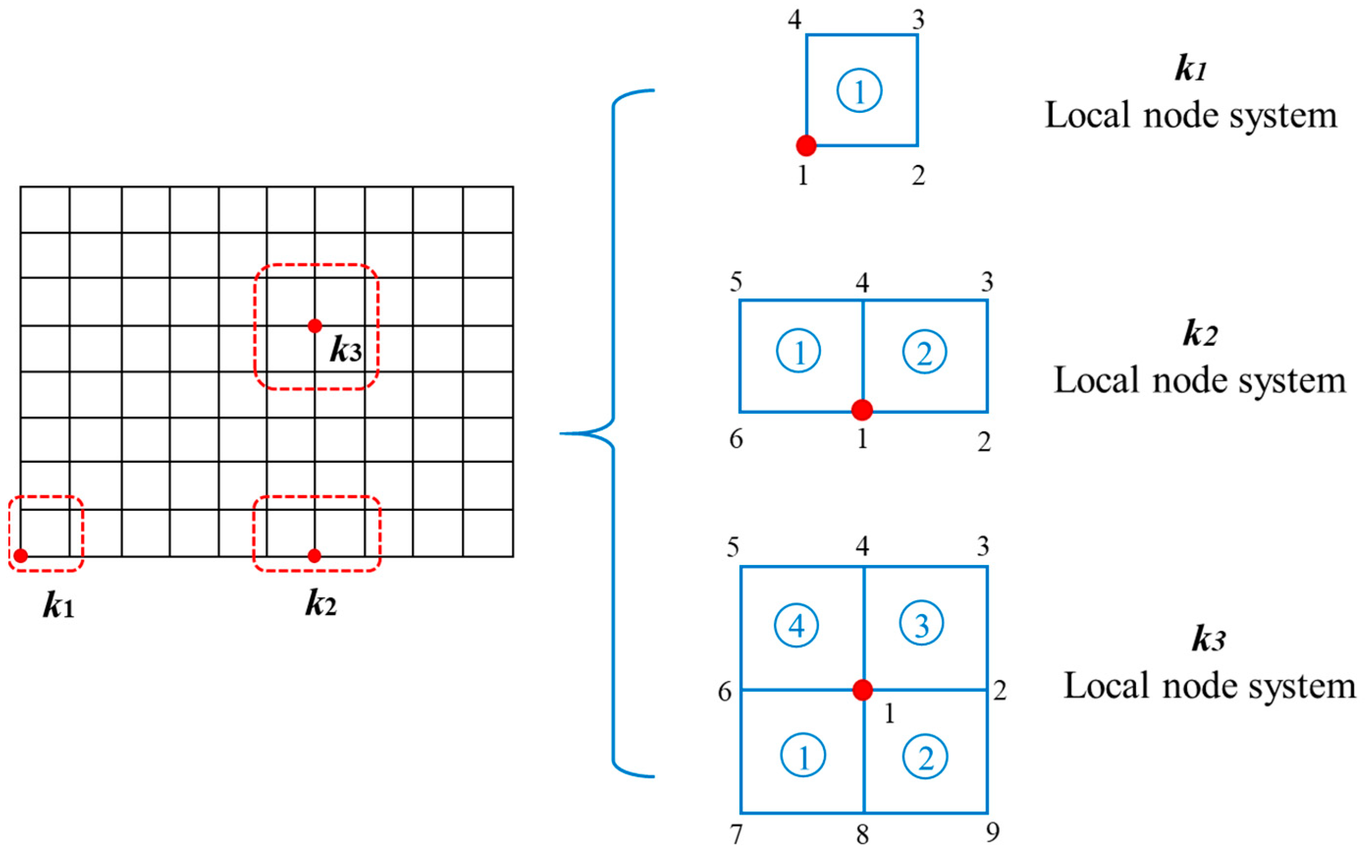
3.1. Spatial Discretization

The dynamic responses of node k only are associated with the responses of the neighboring nodes. On that basis, taking the 2D plane strain problem as an example, the whole computational domain is discretized into local node systems for all nodes [44], as shown in Figure 1. For node k₁ at the corner of the computational domain, the four nodes of element 1 adjacent to node k are renumbered as nodes 1 to 4; similarly, for the node k₂ on the boundary and the node k₃ located inside the computational domain, the local node systems are renumbered by the method shown in Figure 1. In the computational domain, for the local node system composed of any node, an individual finite element equation of the local node system is constructed and is computed in time domain. The dynamic responses for the whole computational domain are obtained by cycling all the nodes.

According to Figure 1, it is assumed that there are n adjacent elements for node k, and each element has four nodes. Based on Equations (6) and (7), the finite element equations of the local node system of node k are expressed as follows:

$${\displaystyle \sum _{L=1}^n{\displaystyle \sum _{j=1}^4{\mathit{M}}_{kj}^L{\ddot{\mathit{u}}}_j^L}}+{\displaystyle \sum _{L=1}^n{\displaystyle \sum _{j=1}^4{\mathit{K}}_{kj}^L{\mathit{u}}_j^L}}-{\displaystyle \sum _{L=1}^n{\displaystyle \sum _{j=1}^4{\mathit{Q}}_{kj}^L{p}_j^L}}={\displaystyle \sum _{L=1}^n{\mathit{f}}_{k,u}^L}$$

(8)

$${\displaystyle \sum _{L=1}^n{\displaystyle \sum _{j=1}^4{S}_{kj}^L{\dot{p}}_j^L}}+{\displaystyle \sum _{L=1}^n{\displaystyle \sum _{j=1}^4{H}_{kj}^L{p}_j^L}}+{\displaystyle \sum _{L=1}^n{\displaystyle \sum _{j=1}^4{\left({\mathit{Q}}_{kj}^L\right)}^T{\dot{\mathit{u}}}_j^L}}={\displaystyle \sum _{L=1}^n{f}_{k,q}^L}$$

(9)

where L represents the influence of the adjacent element L on node k, and j = 1–4 represent the influence of the four nodes of the element L on node k. The matrices in the above equations are defined as follows:

$$\begin{array}{cc}\begin{array}{l}{\mathit{M}}_{ij}^L={\displaystyle {\int }_{-1}^1{\displaystyle {\int }_{-1}^1\rho {\mathit{N}}_{ui}{\mathit{N}}_{uj}}}\left|J\right|d\xi d\eta \\ {\mathit{K}}_{ij}^L={\displaystyle {\int }_{-1}^1{\displaystyle {\int }_{-1}^1{\mathit{N}}_{ui}^T{\mathit{L}}^T\mathit{D}\mathit{L}{\mathit{N}}_{uj}}}\left|J\right|d\xi d\eta \\ {\mathit{Q}}_{ij}^L={\displaystyle {\int }_{-1}^1{\displaystyle {\int }_{-1}^1{\mathit{N}}_{ui}^T\nabla N_{pj}}}\left|J\right|d\xi d\eta \\ H_{ij}^L={\displaystyle {\int }_{-1}^1{\displaystyle {\int }_{-1}^1{\left(\nabla N_{pi}\right)}^T \overline{k}\left(\nabla N_{pj}\right)}}\left|J\right|d\xi d\eta \end{array}& \begin{array}{l}{S}_{ij}^L={\displaystyle {\int }_{-1}^1{\displaystyle {\int }_{-1}^1{N}_{pi}^T\frac{1}{Q_b}{N}_{pj}}}\left|J\right|d\xi d\eta \\ {\mathit{f}}_{i,u}^L={\displaystyle {\int }_{{\mathsf{\Gamma }}^L}{\mathit{N}}_u^T}{\mathit{T}}_{s}dr\\ f_{i,q}^L=-{\displaystyle {\int }_{{\mathsf{\Gamma }}^L}{N}_{\mathrm{p}}^T}{q}_{s}dr\end{array}\end{array}$$

(10)

where M is the mass matrix of saturated porous media, K is the stiffness matrix of the solid phase, Q is the coupling matrix, S is the compressibility matrix of the fluid phase, H is the permeability matrix of the fluid phase, f_u and f_q are the external load of and the flow rate, respectively, T_s is the distributed force on the boundary of element L in the x and y directions, and q_s is the flow rate perpendicular to the boundary of element L.

In fact, Equations (8) and (9) are an alternative expression of Equations (6) and (7). Equations (6) and (7) are the global equations established by assembling the coefficient matrices of the global computational domain. In comparison, Equations (8) and (9) are the equations established for the local node system. The dynamic responses of the whole domain are obtained by cycling all nodes in the computational domain and solving the equation of local node system of each node. Therefore, for the dynamic problem with large degree of freedom, the dimension of equation of the local node system is very small and computational efficiency is higher.

3.2. Explicit Integration Method in Time Domain

To increase the computational efficiency, the finite element Equations (8) and (9) are computed using the explicit integration method [40] in time domain. The equations of the local node system of node k at the t + 1 time step can be expressed as:

$${\mathit{u}}_k^{t+1}=2{\mathit{u}}_k^t-{\mathit{u}}_k^{t-1}+\mathsf{\Delta }{t}^2\frac{1}{{\mathit{M}}_{dk}}{\displaystyle \sum _{L=1}^n{\mathit{f}}_{k,u}^{L,t}}+\mathsf{\Delta }{t}^2\frac{1}{{\mathit{M}}_{dk}}{\displaystyle \sum _{L=1}^n{\displaystyle \sum _{j=1}^4{\mathit{Q}}_{kj}^L{p}_j^{L,t}}}-\mathsf{\Delta }{t}^2\frac{1}{{\mathit{M}}_{dk}}{\displaystyle \sum _{L=1}^n{\displaystyle \sum _{j=1}^4{\mathit{K}}_{kj}^L{\mathit{u}}_j^{L,t}}}$$

(11)

$$p_k^{t+1}=p_k^t+\mathsf{\Delta }t\frac{1}{S_{dk}}{\displaystyle \sum _{L=1}^n{f}_{k,q}^{L,t}}-\frac{1}{S_{dk}}{\displaystyle \sum _{L=1}^n{\displaystyle \sum _{j=1}^4{\left({\mathit{Q}}_{kj}^L\right)}^T}}\left({\mathit{u}}_j^t-{\mathit{u}}_j^{t-1}\right)-\mathsf{\Delta }t\frac{1}{S_{dk}}{\displaystyle \sum _{L=1}^n{\displaystyle \sum _{j=1}^4{H}_{kj}^L{p}_j^{L,t}}}$$

(12)

where the lumped mass matrix ${\mathit{M}}_{dk}^e$ and the lumped fluid compressibility matrix ${\mathit{S}}_{dk}^e$ of element e are processed by the same diagonalization method [40], as shown in Equations (13) and (14).

$${\left({\mathit{M}}_{dk}^e\right)}_{ij}=\{\begin{array}{c}a{\left({\mathit{M}}_k^e\right)}_{ii}=a{\displaystyle \underset{V^e}{\int }{\rho }^e{\mathit{N}}_i^T{\mathit{N}}_{i}d{V}^e} (j=i)\\ 0 (j\ne i)\end{array} , {\displaystyle \sum _{i=1}^{n_e}{\left({\mathit{M}}_{dk}^e\right)}_{ii}}=a{\displaystyle \sum _{i=1}^{n_e}{\left({\mathit{M}}_k^e\right)}_{ii}}=W^e{\mathit{I}}_d={\rho }^e{A}^e{\mathit{I}}_d$$

(13)

$${\left({\mathit{S}}_{dk}^e\right)}_{ij}=\{\begin{array}{c}b{\left({\mathit{S}}_k^e\right)}_{ii}=b{\displaystyle \underset{V^e}{\int }\frac{1}{Q_b^e}{\mathit{N}}_i^T{\mathit{N}}_{i}d{V}^e (j=i)}\\ 0 (j\ne i)\end{array} , {\displaystyle \sum _{i=1}^{n_e}{\left({\mathit{S}}_{dk}^e\right)}_{ii}}=b{\displaystyle \sum _{i=1}^{n_e}{\left({\mathit{S}}_k^e\right)}_{ii}}=V^e{\mathit{I}}_d=\frac{1}{Q_b}{A}^e{\mathit{I}}_d$$

(14)

where ${\mathit{M}}_k^e$ and ${\mathit{S}}_k^e$ are the consistent mass matrix and the consistent fluid compressibility matrix of element e, a and b are corresponding scaling coefficients, W^e and V^e are the mass and compressive deformation of element e, respectively, A^e is the area of element e, and I_d is unit matrix.

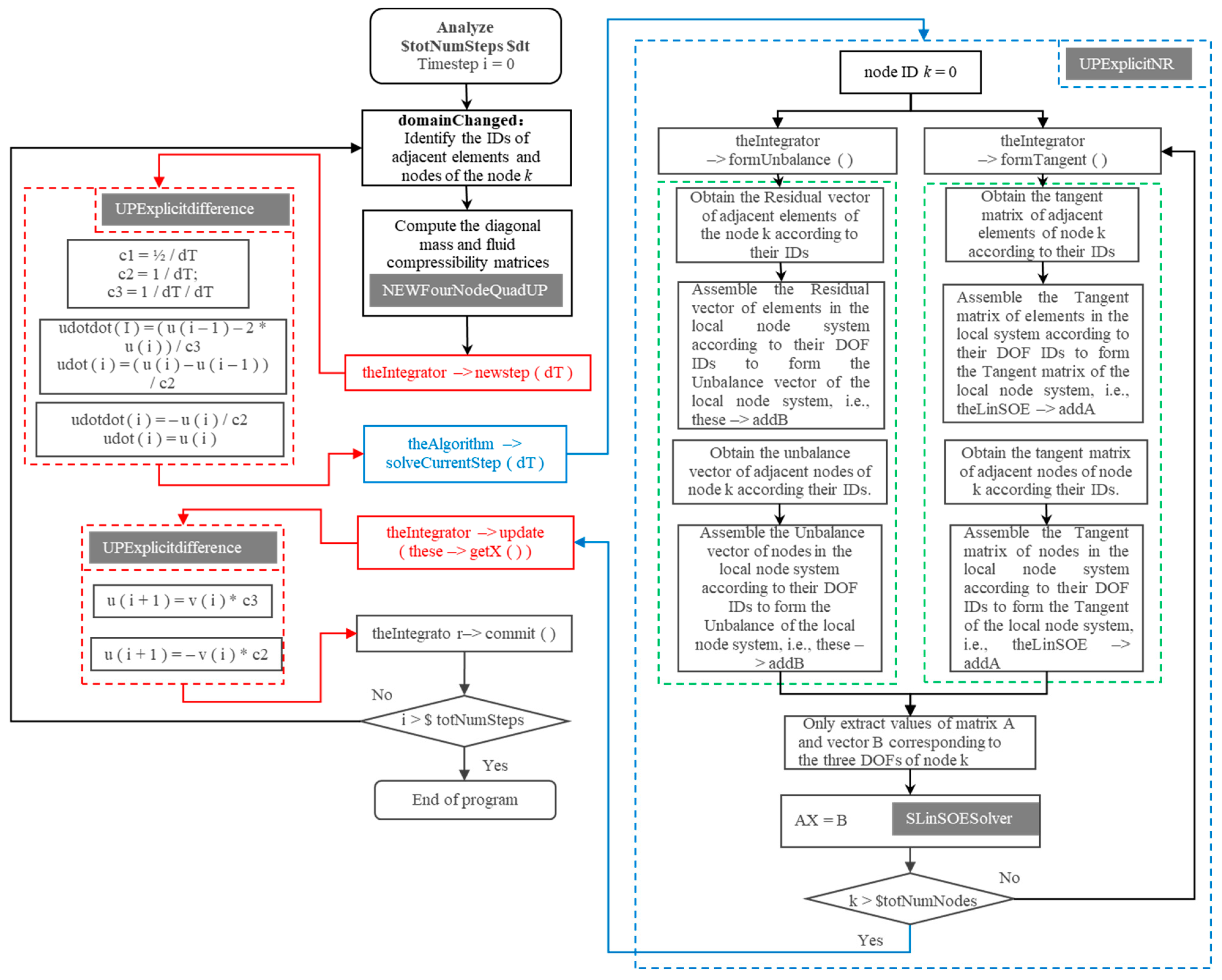
4. Implementation of the Explicit Finite Element Method in OpenSees

The FEM been embedded in the open-source OpenSees software. The calculation does not require solving simultaneous equations but rather solving three uncoupled equations corresponding to the three DOFs (u_kx, u_ky, p) of the node. The dynamic equations AX = B [45,46] can be computed in OpenSees by selecting a suitable algorithm and integrator. The explicit temporal integration method UPExplicitdifference, the algorithm UPExplicitNR, and the equation solver ExplicitLinSOESolver are also added, respectively, and FourNodeQuadUP element for diagonalizing the mass matrix M and fluid compressibility matrix S of elements are added in the software.

The equivalent equations of Equations (11) and (12) are expressed as follows:

$${\tilde{\mathit{K}}}_k {\tilde{\mathit{v}}}_k^{t+1}{}_{} ={\tilde{\mathit{F}}}_k$$

(15)

where

$${\tilde{\mathit{F}}}_k={\mathit{F}}_k-{\mathit{R}}_k-{\overline{\mathit{M}}}_k{\ddot{\tilde{\mathit{v}}}}_{}^t{}_{} -{\overline{\mathit{C}}}_k{\dot{\tilde{\mathit{v}}}}_{}^t{}_{}$$

(16)

$${\tilde{\mathit{K}}}_k=\left[\begin{array}{cc}{\mathit{M}}_{dk}& \mathbf{0}\\ \mathbf{0}& -S_{dk}\end{array}\right],{\overline{\mathit{C}}}_k=\left[\begin{array}{cc}\mathbf{0}& -{\mathit{Q}}_k\\ -{\mathit{Q}}_k^T& -H_k\end{array}\right],{\mathit{F}}_k=\left\{\begin{array}{c}{\mathit{f}}_{uk}^t\\ -f_{qk}^t\end{array}\right\}$$

(17)

$${\tilde{\mathit{v}}}_k^{t+1}{}_{} =\left\{\begin{array}{c}\frac{{\mathit{u}}_k^{t+1} }{\mathsf{\Delta }{t}^2}\\ \frac{p_k^{t+1}}{\mathsf{\Delta }t}\end{array}\right\},{\dot{\tilde{\mathit{v}}}}_{}^t{}_{} =\left\{\begin{array}{c}\frac{{\mathit{u}}_{}^t-{\mathit{u}}_{}^{t-1}}{\mathsf{\Delta }t}\\ p_{}^t\end{array}\right\},{\ddot{\tilde{\mathit{v}}}}_{}^t{}_{} =\left\{\begin{array}{c}\frac{{\mathit{u}}_{}^{t-1}-2{\mathit{u}}_{}^t}{\mathsf{\Delta }{t}^2}\\ -\frac{p_{}^t}{\mathsf{\Delta }t}\end{array}\right\}$$

(18)

where $\tilde{\mathit{K}}$ in Equation (15) is a diagonal matrix. The dynamic responses of node k are calculated by only the three equations corresponding to the three DOFs (u_xk, u_yk, p_k) in Equation (15):

$$\{\begin{array}{c}{M}_{dk,x} {\tilde{v}}_{k,x}^{t+1}{}_{} ={\tilde{F}}_{k,x}\\ M_{dk,y} {\tilde{v}}_{k,y}^{t+1}{}_{} ={\tilde{F}}_{k,y}\\ -S_{dk} {\tilde{v}}_{k,p}^{t+1}{}_{} ={\tilde{F}}_{k,p}\end{array}$$

(19)

Equation (19) is the equivalent form to Equations (11) and (12). The displacements and pore pressure of the node k at time t + 1 are obtained by Equation (19).

$$\left\{\begin{array}{c}{u}_{k,x}^{t+1} \\ u_{k,y}^{t+1} \\ p_k^{t+1}\end{array}\right\}=\left\{\begin{array}{c}\mathsf{\Delta }{t}^2\cdot {\tilde{v}}_{k,x}^{t+1}{}_{} \\ \mathsf{\Delta }{t}^2\cdot {\tilde{v}}_{k,y}^{t+1}{}_{} \\ \mathsf{\Delta }t\cdot {\tilde{v}}_{k,p}^{t+1}{}_{} \end{array}\right\}$$

(20)

The dynamic responses of the global domain at any time can be obtained by solving of Equation (19) of all nodes. The computational flowchart of the proposed explicit FEM in OpenSees is shown in Figure 2. In space domain, the proposed algorithm UPExplicitNR is used to construct individual finite element equation of the local node system, and results of the whole system are obtained by cycling all the nodes based on UPExplicitNR. In time domain, the explicit temporal integration method UPExplicitdifference is used to compute the results in every time step.

The proposed algorithm has a much lower computational efficiency than implicit methods for problems with a small DOFs. However, for the problems with a large DOFs or strong nonlinear problems, the proposed method does not require the solving of simultaneous equations, only computing three decoupled equations for each node, and no nonlinear iterative computation is performed within a suitable time step. Therefore, the efficiency of the proposed method is improved significantly, and the computational memory is saved.

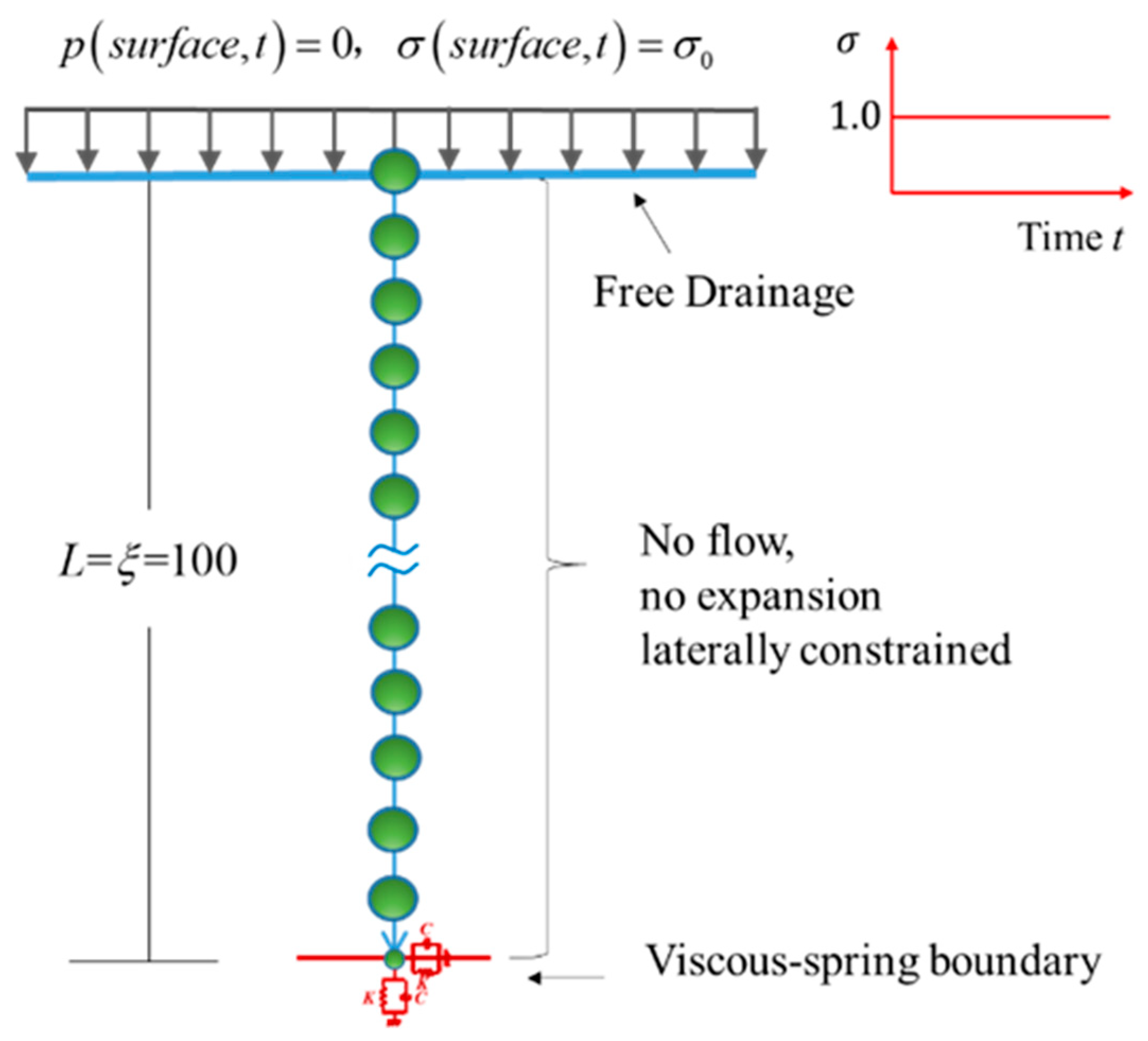
5. Viscoelastic Artificial Boundary

For the problems of wave propagation in saturated porous media, a viscoelastic artificial boundary for the u-p equations is adopted. It is expressed as follows:

$${\mathit{f}}_{uBl}=-{\mathit{K}}_{Bl}^{\infty }{\mathit{u}}_{Bl}-{\mathit{C}}_{Bl}^{\infty }{\dot{\mathit{u}}}_{Bl}-{\mathit{Q}}_{Bl}^{\infty }{p}_{Bl}$$

(21)

$$f_{qBl}=H_{Bl}^{\infty }{p}_{Bl}+S_{Bl}^{\infty }{\dot{p}}_{Bl}$$

(22)

where ∞ denotes the exterior domain, Bl is the node l on the boundary, ${\mathit{f}}_{uBl}^{}$ and $f_{qBl}^{}$ are the stress and flow velocity of the node l on the boundary, respectively, and ${\mathit{u}}_{Bl}^{}$ and $p_{Bl}^{}$ are the displacement and pore pressure of the node l on the boundary, respectively. The coefficients in the above equations are expressed as follows:

$$\begin{gathered} {\mathit{K}}_{Bl}^{\infty }={\mathit{W}}^T{L}_l\left[\begin{array}{cc}{K}_{BN}^{\infty }& 0\\ 0& K_{BT}^{\infty }\end{array}\right]\mathit{W}; {\mathit{C}}_{Bl}^{\infty }={\mathit{W}}^T{L}_l\left[\begin{array}{cc}{C}_{BN}^{\infty }& 0\\ 0& C_{BT}^{\infty }\end{array}\right]\mathit{W}; \\ {\mathit{Q}}_{Bl}^{\infty }={\mathit{W}}^T{L}_l\left[\begin{array}{c}{Q}_B^{\infty }\\ 0\end{array}\right] \end{gathered}$$

(23)

$$H_{Bl}^{\infty }=L_l{H}_B^{\infty }{S}_{Bl}^{\infty }=L_l{S}_B^{\infty }$$

(24)

where L_l is the length corresponding to node l on the boundary, and W is the coordinate transformation matrix for transforming the local coordinates to the global coordinates. The parameters in the above equations are specifically

$$\mathit{W}=\left[\begin{array}{cc}{l}_{rx}& l_{ry}\\ l_{\perp x}& l_{\perp y}\end{array}\right]$$

(25)

$$K_{BN}^{\infty }=\frac{\lambda +2G}{2r\left(1+A\right)}; K_{BT}^{\infty }=\frac{G}{2r\left(1+A\right)}$$

(26)

$$C_{BN}^{\infty }=B\rho C_{P1}^r; C_{BT}^{\infty }=B\rho C_S^r$$

(27)

$$Q_B^{\infty }=\alpha ; H_B^{\infty }=\frac{\overline{k}}{2r\left(1+A\right)}; S_B^{\infty }=\frac{\overline{k}}{C_{P1}^r}$$

(28)

In Equation (25), $l_{rx}=\cos (r,x)$ is the cosine of the angle between the positive direction of the local r axis and the positive direction of the global x-axis. Other parameters in Equation (25) are defined similarly to l_xy. A = 0.8 and B = 1.1.

The artificial boundary condition as shown in Equations (21) and (22) actually changes only the diagonal values of the coefficient matrix corresponding to boundary nodes in local node system. Assume that there are m nodes on the boundary in the local node system of node k. Equations (21) and (22) are substituted into Equations (8) and (9) to obtain the finite element equations considering the viscoelastic artificial boundary:

$${\mathit{M}}_{dk}^{}{\ddot{\mathit{u}}}_k+{\displaystyle \sum _{l=1}^m{\mathit{C}}_{Bl}^{\infty }{\dot{\mathit{u}}}_{Bl}}+\left({\displaystyle \sum _{L=1}^n{\displaystyle \sum _{j=1}^4{\mathit{K}}_{kj}^L{\mathit{u}}_j^L+{\displaystyle \sum _{l=1}^m{K}_{Bl}^{\infty }{u}_{Bl}}}}\right)-\left({\displaystyle \sum _{L=1}^n{\displaystyle \sum _{j=1}^4{\mathit{Q}}_{kj}^L{p}_j^L-{\displaystyle \sum _{l=1}^m{\mathit{Q}}_{Bl}^{\infty }{p}_{Bl}}}}\right)={\displaystyle \sum _{L=1}^n{\mathit{f}}_{k,u}^L}$$

(29)

$$\left(S_{dk}^{}{\dot{p}}_k^{}+{\displaystyle \sum _{l=1}^m{S}_{Bl}^{\infty }{\dot{p}}_{Bl}}\right)+\left({\displaystyle \sum _{L=1}^n{\displaystyle \sum _{j=1}^4{H}_{kj}^L{p}_j^L}}+{\displaystyle \sum _{l=1}^m{H}_{Bl}^{\infty }{p}_{Bl}}\right)+{\displaystyle \sum _{L=1}^n{\displaystyle \sum _{j=1}^4{\left({\mathit{Q}}_{kj}^L\right)}^T{\dot{\mathit{u}}}_j^L}}={\displaystyle \sum _{L=1}^n{f}_{k,q}^L}$$

(30)

Compared to Equation (8), Equation (29) has an additional damping term and can be solved by an explicit integration method [47], and the equations of the local node system of node k at the t + 1 time step can be expressed as:

$$\begin{array}{l}{\mathit{u}}_k^{t+1}={\mathit{u}}_k^t+\frac{\mathsf{\Delta }{t}^2}{2}\frac{1}{{\mathit{M}}_{dk}}{\displaystyle \sum _{L=1}^n{\mathit{f}}_{k,u}^{L,t}}+\frac{\mathsf{\Delta }{t}^2}{2}\frac{1}{{\mathit{M}}_{dk}}\left({\displaystyle \sum _{L=1}^n{\displaystyle \sum _{j=1}^4{\mathit{Q}}_{kj}^L{p}_j^L-{\displaystyle \sum _{l=1}^m{\mathit{Q}}_{Bl}^{\infty }{p}_{Bl}}}}\right)-\frac{\mathsf{\Delta }{t}^2}{2}\frac{1}{{\mathit{M}}_{dk}}\left({\displaystyle \sum _{L=1}^n{\displaystyle \sum _{j=1}^4{\mathit{K}}_{kj}^L{\mathit{u}}_j^L+{\displaystyle \sum _{l=1}^m{\mathit{K}}_{Bl}^{\infty }{\mathit{u}}_{Bl}}}}\right)\\ +\frac{\mathsf{\Delta }t}{2}\frac{1}{{\mathit{M}}_{dk}}{\displaystyle \sum _{l=1}^m{\mathit{C}}_{Bl}^{\infty }{\mathit{u}}_{Bl}^t}-\frac{\mathsf{\Delta }t}{2}\frac{1}{{\mathit{M}}_{dk}}{\displaystyle \sum _{l=1}^m{\mathit{C}}_{Bl}^{\infty }{\mathit{u}}_{Bl}^{t-1}}-\mathsf{\Delta }{t}^2\frac{1}{{\mathit{M}}_{dk}}{\displaystyle \sum _{l=1}^m{\mathit{C}}_{Bl}^{\infty }{\dot{\mathit{u}}}_{Bl}^t}+\mathsf{\Delta }t{\dot{\mathit{u}}}_{Bk}^t\end{array}$$

(31)

$$p_k^{t+1}=p_k^t+\frac{\mathsf{\Delta }t}{S_{dk}+S_{Bk}^{\infty }}{\displaystyle \sum _{L=1}^n{f}_{k,q}^{L,t}}-\frac{1}{S_d+S_{Bk}^{\infty }}{\displaystyle \sum _{L=1}^n{\displaystyle \sum _{j=1}^4{\left({\mathit{Q}}_{kj}^L\right)}^T}}\left({\mathit{u}}_j^t-{\mathit{u}}_j^{t-1}\right)-\frac{\mathsf{\Delta }t}{S_d+S_{Bk}^{\infty }}\left({\displaystyle \sum _{L=1}^n{\displaystyle \sum _{j=1}^4{H}_{kj}^L{p}_j^L}}+{\displaystyle \sum _{l=1}^m{H}_{Bl}^{\infty }{p}_{Bl}}\right)$$

(32)

where, the subscript Bk of ${\dot{\mathit{u}}}_{Bk}^t$ and $S_{Bk}^{\infty }$ represents the corresponding value when the target node k is also the node on the boundary.

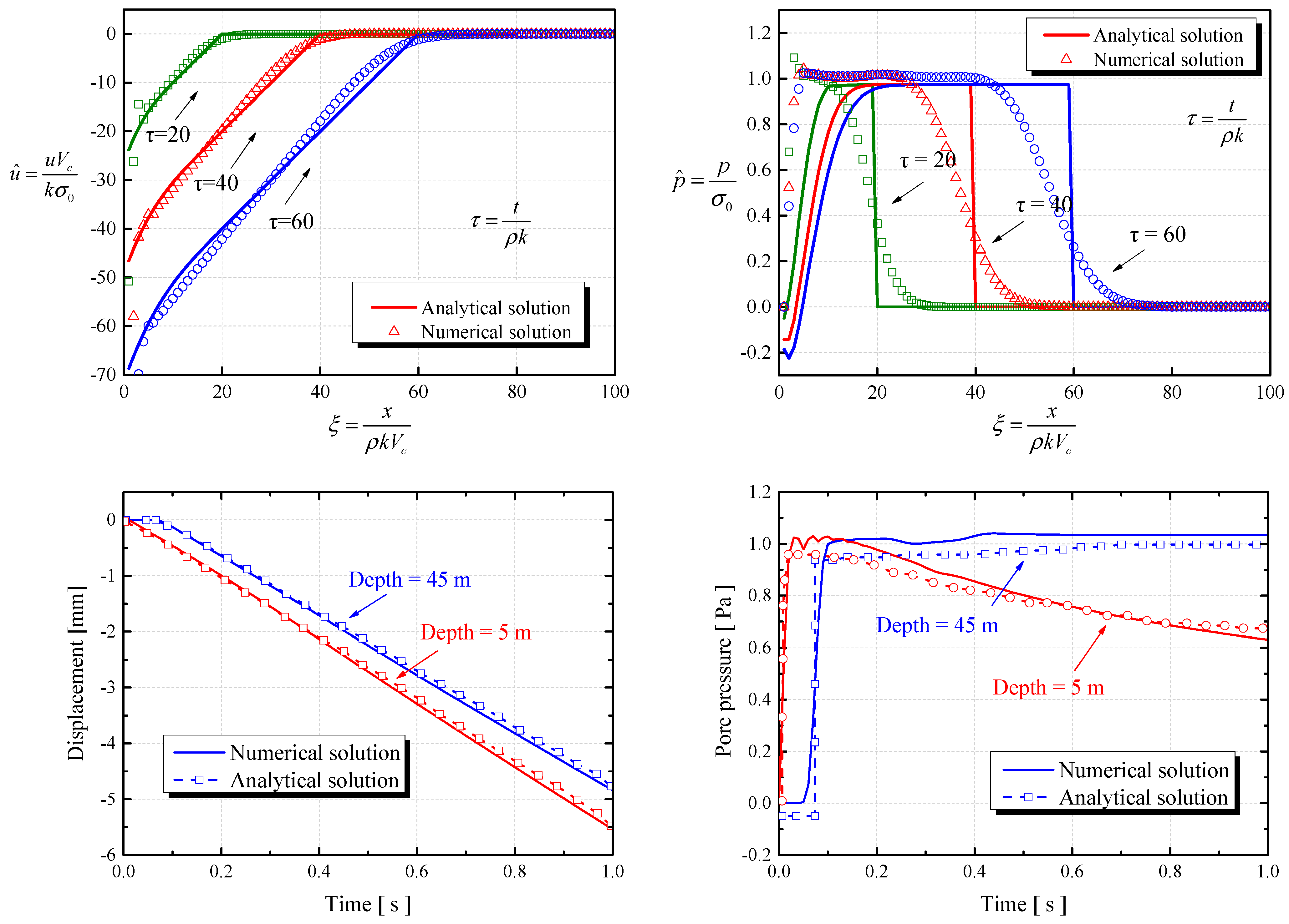
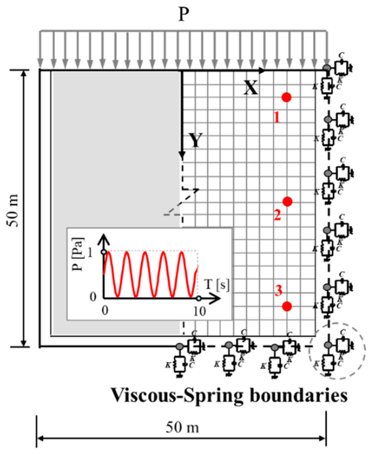
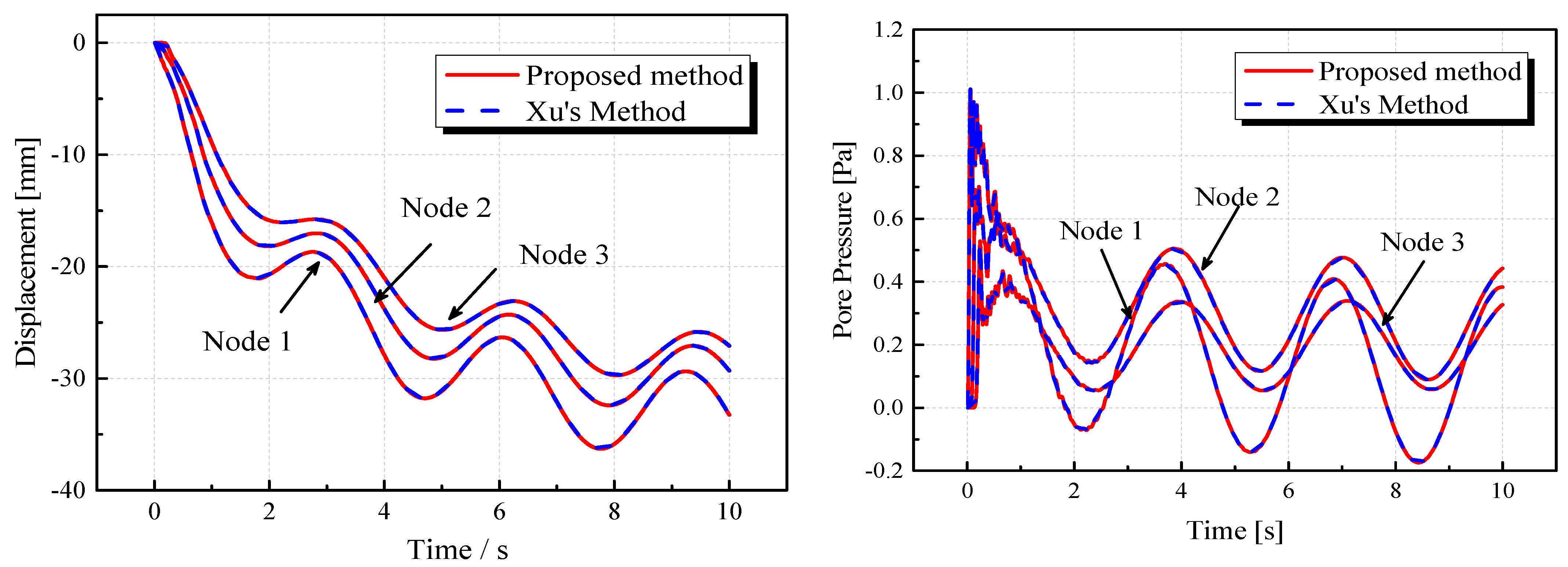
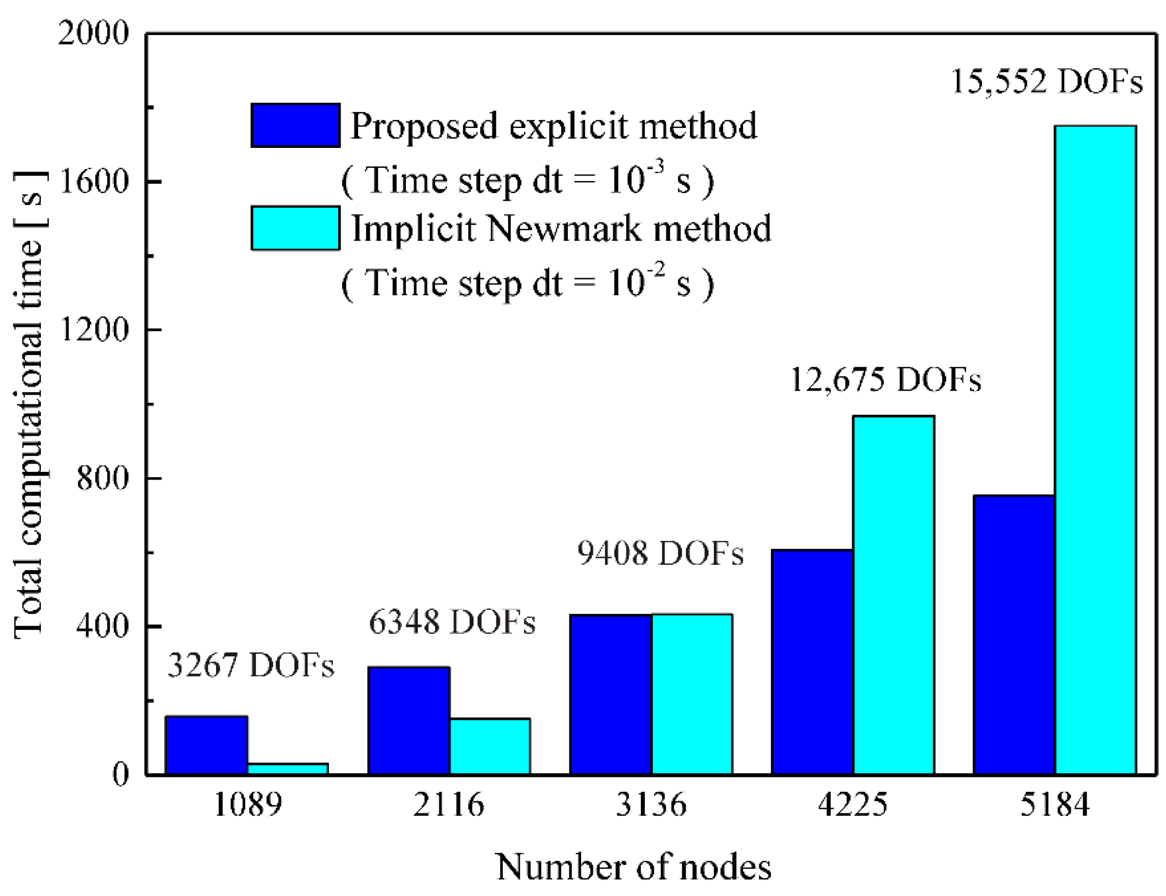
6. Validation of Method and Comparison of Computational Efficiency

Example 1.

The computational model for a one-dimensional (1D) semi-infinite domain of saturated porous media is shown in Figure 3. The left and right sides of the model are impermeable boundaries, and their horizontal displacement is fixed. The bottom of the model is assigned a viscoelastic artificial boundary, and the top surface of the model is a free drainage boundary applied with a constant uniform load of 1.0 Pa. The material parameters of the model listed in

Table 1. Parameters of linear elastic saturated soil.

Basic Material Parameters
Parameter	Value
ES	3000 Pa		Young’s modulus
ρ	0.306 kg/m3		Density of two-phase media
ρf	0.2977 kg/m3		Density of fluid-phase
n	0.333		Porosity
ν	0.2		Poisson’s ratio
$\overline{k}$	0.004883 m3s/kg		Dynamic permeability coefficient
λ	833.3 Pa		Lame’s constants of the soil skeleton
G	1250 Pa		Shear modulus
Variable material parameters considered in the example
Parameter Parameters	No. 1	No. 2
Kf	0.3999 × 105 Pa	0.6106 × 105 Pa	Bulk modulus of pore fluid
Ks	∞	0.5005 × 104 Pa	Bulk modulus of soil skeleton
Qb	0.1201 × 106 Pa	0.1385 × 105 Pa	Compressibility coefficient of pore fluid
Wave propagation velocity in saturated soil
Parameter	Actual wave velocity
	No. 1	No. 2
Cp	635.12 m/s	176.15 m/s	P wave velocity
Cs	63.92 m/s	89.69 m/s	S wave velocity

[21,48] as Material No. 1 are taken from the reference [21,48]. The analytical solutions, as the reference solutions, for the 1D problem of saturated porous media proposed by Simon et al. [21].

In Figure 4, the numerical solutions and analytical solutions are compared at three dimensionless time parameter τ = 20, 40, and 60, respectively. The numerical solutions of the displacement and pore pressure of the 1D soil column are in relatively good agreement with the analytical solutions. In addition, the numerical and analytical solutions of the displacement and pore pressure dynamic time-history responses at nodes 5 m and 45 m from the center of the load are compared in Figure 4, which shows consistency between the two results. The comparison results verify the accuracy of proposed method.

Example 2.

Computational efficiency is compared in this example. A 2D computational model with size of 50 m × 50 m is shown in Figure 5. The top surface of the model is set as a drainage boundary and is subjected to a uniformly distributed sinusoidal load, and each of the other three sides are set as artificial boundaries. Three target nodes (1, 2, and 3) are selected for analysis. The material properties are listed in Table 1 as Material No. 2. Xu’s method and Newmark method are used to compare the responses and computational efficiency with the proposed method, respectively.

Figure 6 shows the displacement and pore pressure time-history curves of the target nodes. The red and blue curves in the figure represent the results obtained from the proposed method and the Xu’s method [40], respectively. The results of the two methods have a good consistence. The consistency further validates the proposed method.

By refining grids of the model in Figure 5, the total computational times of the proposed method and Newmark [31] method are compared in Figure 7. The model is discretized into approximately 1000, 2000, 3000, 4000, and 5000 nodes, respectively. Comparison of the computation time of the two algorithms show that when the model has a relatively small number of nodes, the implicit Newmark method leads to much less computation time than the proposed method, because it is unconditionally stable and allows a relatively large time step. However, as the number of nodes increases to approximately 3000, the total computation time of the two methods is basically similar, and the computational efficiency of the proposed method is significantly improved. When the number of nodes increases to approximately 4000, the computational efficiency of the proposed explicit method is far higher than the implicit Newmark method, and such an advantage becomes more significant as the number of nodes continues to increase.

7. Analysis of Nonlinear Problems

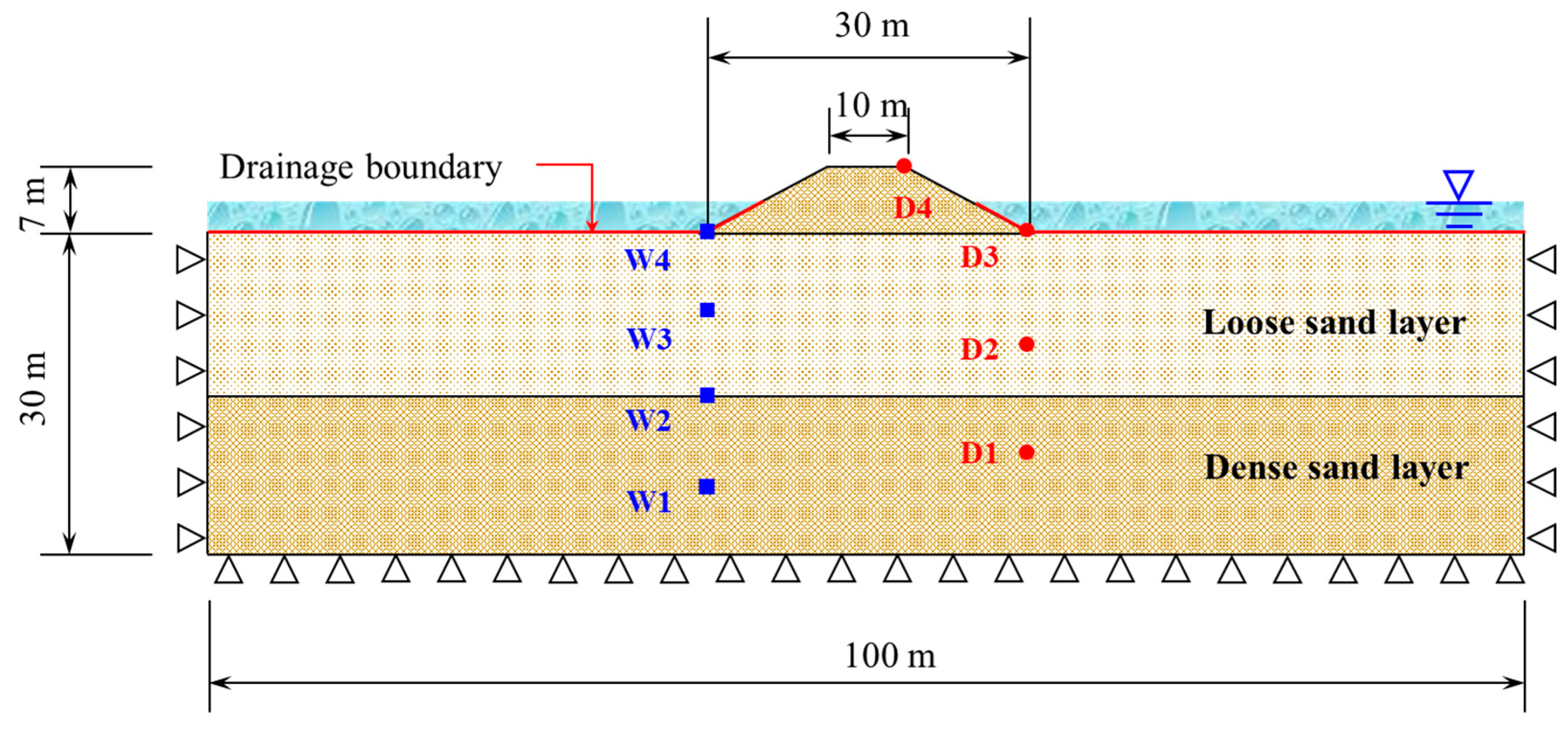
7.1. Finite Element Model

Figure 8 shows the 2D model of a liquefiable site, which is composed of a 15 m dense sand layer, a 15 m liquefiable loose sand layer, and an 8 m-dense sand embankment from bottom to top. The seawater has a depth of 2 m. The top surface of the model is set as a drainage boundary. To simplify the model, the horizontal and vertical displacements at the bottom of the model are fixed, and the horizontal displacements of the left and right side boundaries are also fixed.

The Wolong station seismic record of the Wenchuan earthquake is selected as the input motion. It has a peak acceleration of 0.3 g. The acceleration time history curve is shown in Figure 9. Attention is fixed on the numerical results at 6.2 s, 16.6 s, and 30 s, respectively.

The saturated soils are simulated using the quadrilateral plane strain element element quadUP [49,50]. The parameters of soil elements are listed in

Table 2. Soil element parameters.

	Loose Sand Layer	Dense Sand Layer
Element thickness	1.0 m	1.0 m
Vertical gravitational acceleration	−9.81 m/s2	−9.81 m/s2
Liquid-phase undrained bulk modulus	4.4 × 106 kPa	7.3 × 106 kPa
Horizontal permeability coefficient	1 × 10−4 m/s	1 × 10−5 m/s
Vertical permeability coefficient	1 × 10−4 m/s	1 × 10−5 m/s

. Each node of the element has three DOFs, corresponding to horizontal displacement, vertical displacement, and pore pressure, respectively. In view of using a 2D plane strain model to simulate a 3D problem, the out of plane thickness of the model is set to be 1.0 m. The constitutive model of saturated soil chooses the PressureDependMutiYield02 (PDMY) command [51,52], with the material parameters [49] listed in

Table 3. Material parameters of the model.

Parameters	Loose Sand Layer	Dense Sand Layer
$\mathrm{Density} \rho$	1.7 ton/m3	1.9 ton/m3
$\mathrm{Reference} \mathrm{shear} \mathrm{modulus} G_r$	3.57 × 104 kPa	2.59 × 104 kPa
$\mathrm{Reference} \mathrm{bulk} \mathrm{modulus} B_r$	8 × 104 kPa	6 × 104 kPa
$\mathrm{Friction} \mathrm{angle} \varphi$	33.5	31
$\mathrm{Octahedral} \mathrm{peak} \mathrm{shear} \mathrm{strain} {\gamma }_{\max }$	0.1	0.1
Pressure coefficient n	0.5	0.5
$\mathrm{Dilatancy} \mathrm{angle} {\varphi }_{PT}$	25.5	31
$\mathrm{Shear} \mathrm{contraction} \mathrm{coefficient} c_1$	0.045	0.087
$\mathrm{Shear} \mathrm{contraction} \mathrm{coefficient} c_3$	0.15	0.18
$\mathrm{Dilatancy} \mathrm{coefficient} d_1$	0.06	0.0
$\mathrm{Dilatancy} \mathrm{coefficient} d_3$	0.15	0.0
Number of yield surface	20	20
$\mathrm{Shear} \mathrm{contraction} \mathrm{coefficient} c_2$	5	5
$\mathrm{Dilatancy} \mathrm{coefficient} d_2$	3	3
$\mathrm{Liquefaction} \mathrm{coefficient} l_1$	1 kPa	1 kPa
$\mathrm{Liquefaction} \mathrm{coefficient} l_2$	0.0	0.0
Initial void ratio e	0.6	0.6
Cs 1	0.9	0.9
Cs2	0.02	0.02
Cs 3	0.7	0.7
Standard pressure	101	101

.

7.2. Numerical Results and Analysis

The seismic responses of the saturated porous media are analyzed by the proposed method and the implicit Newmark method, respectively. Figure 10 shows the time history curves of horizontal and vertical displacements at measuring points D1–D4. The horizontal displacement and vertical displacement at each measuring point gradually increase with time and gradually decrease with burial depth, and reach the maximum of 0.1 m and 0.12 m, respectively, at the top of the embankment. In addition, the time history curves of both horizontal and vertical displacement show the stepwise increase in amplitude, respectively, at 6.2 s and 16.6 s.

Figure 11 shows the excess pore pressure time history curves at measuring points W1–W4. These curves exhibit basically the same variation trends, and their peaks occur at basically consistent time points. The amplitude of pore pressure at each measuring point gradually increases with the increase in the burial depth. The excess pore pressure of the dense sand layer reaches a maximum value of 75 kPa.

Moreover, Figure 10 and Figure 11 compare the results of the proposed method and the implicit Newmark method. The comparison shows that the numerical results of each measuring point obtained by the two methods agree well, indicating the correctness of the proposed method.

To observe the overall lateral deformation and settlement of the site, Figure 12 shows the contour plots of horizontal displacement of the site at 6.2 s, 16.6 s, and 30.0 s, as well as the contour plots of vertical displacement at 30 s. The deformation in the figure is magnified 30 times. As can be seen from the figure, the horizontal displacement at the nodes on the left and right sides of the embankment is the largest; the embankment gradually collapses under the earthquake, causing the embankment soil to move toward both sides, with the maximum horizontal and vertical displacements reaching 0.13 m and 0.19 m, respectively, at 30 s.

Figure 13 shows the contour plots of pore pressure ratios of the ground soil. The loose sand layer near the drainage boundary liquefies at 6.2 s and 16.6 s. As the decrease in the input acceleration, the pore water is drained upwards, and the soil particles are redistributed. The soil tends to a stable state.

Figure 12 and Figure 13 also compare the contour plots of displacement and pore pressure ratio computed by the proposed method and the implicit Newmark implicit method, respectively. The soil deformation patterns obtained by the two methods are similar, and the magnitudes of displacement and pore pressure computed by the two methods are basically consistent, further validating the correctness of the proposed method.

8. Conclusions

An explicit FEM for solving the dynamic responses of saturated porous media is proposed based on the u-p formulation. In spatial domain, the global system is divided into the local node systems of all nodes, which means that the responses of each node only are related to the responses of the surrounding nodes. In time domain, the local node system of each node can be discretized by a completed explicit integration method, and further be simplify into three independent equations corresponding to each DOF of the node. The dimension of FE equations of each local node system is small and is solved fast. By cycling through all the nodes, the dynamic responses of the global computational domain can be obtained. In this way, the proposed method has the high efficiency for solving larger DOFs problem and strong nonlinear problem of the fluid-saturated porous media. Moreover, a viscoelastic artificial boundary is added to the method, and changes only the diagonal values of the coefficient matrix corresponding to boundary nodes and does not change the form of each coefficient matrix corresponding to each local node system. Additionally, the proposed method is validated by comparing with the analytical and numerical solutions of existing methods, and it has high computational efficiency. In the end, the application to the seismic responses of liquefiable site indicates that the proposed method is an effective method for solving the dynamic problems of saturated porous media.

In this method, a complete explicit integration method with only first-order accuracy is chosen. However, based on the same spatial discretization, other suitable integration methods with high order accuracy can also be used in the FE method, such as the integration method used in the viscoelastic artificial boundary section. In addition, the computational efficiency of the proposed method only is verified by comparing with implicit Newmark method. The generality of the proposed needs to be confirmed for various types of analyses and comparisons.

References

1. Houmadi, Y.; Benmoussa, M.Y.C.; Cherifi, W.N.E.H.; Rahal, D.D. Probabilistic analysis of consolidation problems using subset simulation. Comput. Geotech. 2020, 124, 103612. [Google Scholar] [CrossRef]
2. Savvides, A.A.; Papadrakakis, M. A probabilistic assessment for porous consolidation of clays. SN Appl. Sci. 2020, 2, 2115. [Google Scholar] [CrossRef]
3. Ahmed, A.; Soubra, A.H. Probabilistic analysis of strip footings resting on a spatially random soil using subset simulation approach. Georisk Assess. Manag. Risk Eng. Syst. Geohazards 2012, 6, 188–201. [Google Scholar] [CrossRef] [Green Version]
4. Savvides, A.A.; Papadrakakis, M. A computational study on the uncertainty quantification of failure of clays with a modified Cam-Clay yield criterion. SN Appl. Sci. 2021, 3, 659. [Google Scholar] [CrossRef]
5. Mercado, V.; Ochoa-Cornejo, F.; Astroza, R.; El-Sekelly, W.; Abdoun, T.; Pastén, C.; Pastén, F. Uncertainty quantification and propagation in the modeling of liquefiable sands. Soil Dyn. Earthq. Eng. 2019, 123, 217–229. [Google Scholar] [CrossRef]
6. Najjar, S.S.; Sadek, S.; Alcovero, A. Quantification of model uncertainty in shear strength predictions for fiber-reinforced sand. J. Geotech. Geoenviron. Eng. 2013, 139, 116–133. [Google Scholar] [CrossRef]
7. Zienkiewicz, O.C.; Chan, A.H.C.; Pastor, M.; Paul, D.K.; Shiomi, T. Static and dynamic behaviour of soils: A rational approach to quantitative solutions. I. Fully saturated problems. Proc. R. Soc. Lond. A Math. Phys. Eng. Sci. R. Soc. 1990, 429, 285–309. [Google Scholar]
8. Zienkiewicz, O.C.; Taylor, R.L. The Finite Element Method; McGraw-Hill: London, UK, 1977. [Google Scholar]
9. Marcuson, W.F. Definition of terms related to liquefaction. J. Geotech. Eng. Div. 1978, 104, 1197–1200. [Google Scholar]
10. Tang, L. Study on p-y Curve Models for Pile-Soil Dynamic Interactions in Liquefied Ground; Harbin Institute of Technology: Harbin, China, 2010. (In Chinese) [Google Scholar]
11. Mori, S.; Namuta, A.; Miwa, S. Feature of liquefaction damage during the 1993 Hokkaido Nanseioki earthquake. In Proceedings of the 29th Annual Conference of Japanese Society of Soil Mechanics and Foundation Engineering, New Delhi, India, June 1994; pp. 1005–1008. [Google Scholar]
12. Cao, Z.; Hou, L.; Yuan, X.; Sun, R.; Wang, W.; Chen, L. Characteristics of liquefaction-induced damages during Wenchuan Ms 8.0 earthquake. Rock Soil Mech. 2010, 31, 3549–3555, (In Chinese with English Abstract). [Google Scholar]
13. Cao, Z.; Youd, T.L.; Yuan, X. Gravelly soils that liquefied during 2008 Wenchuan, China earthquake, Ms = 8.0. Soil Dyn. Earthq. Eng. 2011, 31, 1132–1143. [Google Scholar] [CrossRef]
14. Huang, Y.; Jiang, X.M. Field-observed phenomena of seismic liquefaction and subsidence during the 2008 Wenchuan earthquake. Nat. Hazards 2010, 54, 839–850. [Google Scholar] [CrossRef]
15. Ishihara, K.; Yasuda, S.; Yoshida, Y. Liquefaction-induced flow failure of embankment and residual strength of silty sand. Soils Found 1990, 30, 69–80. [Google Scholar] [CrossRef] [Green Version]
16. Hamada, M.; Sato, H.; Kawakami, T. A consideration of the mechanism for liquefaction-related large ground displacement. In Proceedings of the Fifth U.S.–Japan Workshop on Earthquake Resistant Design of Lifeline Facilities and Countermeasures Against Soil Liquefaction, Salt Lake City, UT, USA, 29 September–1 October 1994; pp. 217–232. [Google Scholar]
17. Finn, W.D.L.; Fujita, N. Piles in liquefiable soils: Seismic analysis and design issues. Soil Dyn. Earthq. Eng. 2002, 22, 731–742. [Google Scholar] [CrossRef]
18. Biot, M.A. General solutions of the Equations of elasticity and consolidation for a porous material. Appl. Mech. 1956, 23, 91–96. [Google Scholar] [CrossRef]
19. Biot, M.A. Theory of propagation of elastic waves in a fluid-saturated porous solid. I. Low-frequency range. Acoust. Soc. Am. 1956, 28, 168–178. [Google Scholar] [CrossRef]
20. Zienkiewicz, O.C.; Chang, C.T.; Bettess, P. Drained, undrained, consolidating, and dynamic behavior assumptions in soils: Limits of validity. Geotechnique 1980, 30, 385–395. [Google Scholar] [CrossRef]
21. Simon, B.R.; Zienkiewicz, O.C.; Paul, D.K. An analytical solution for the transient response of saturated porous elastic solids. Numer. Anal. Methods Geomech. 1984, 8, 381–398. [Google Scholar] [CrossRef]
22. Newmark, N.M. A method of computation for structural dynamics. J. Eng. Mech. Div. 1959, 85, 67–94. [Google Scholar] [CrossRef]
23. Wilson, E.L.; Farhoomand, I.; Bathe, K.J. Nonlinear dynamic analysis of complex structures. Earthq. Eng. Struct. Dyn. 1972, 1, 241–252. [Google Scholar] [CrossRef]
24. Chung, J.; Hulbert, G.M. A time integration algorithm for structural dynamics with improved numerical dissipation. Gen.-Method J. Appl. Mech. 1993, 60, 371–375. [Google Scholar] [CrossRef]
25. Kontoe, S.; Zdravkovic, L.; Potts, D.M. An assessment of time integration schemes for dynamic geotechnical problems. Comput. Geotech. 2008, 35, 253–264. [Google Scholar] [CrossRef] [Green Version]
26. Zhao, C.; Li, W.; Wang, J. An explicit finite element method for Biot dynamic formulation in fluid-saturated porous media and its application to a rigid foundation. J. Sound Vib. 2005, 282, 1169–1181. [Google Scholar] [CrossRef]
27. Wang, J.; Zhang, C.; Du, X. An explicit integration scheme for solving dynamic problems of solid and porous media. J. Earthq. Eng. 2008, 12, 293–311. [Google Scholar] [CrossRef]
28. Simon, B.R.; Wu, J.S.S.; Zienkiewicz, O.C.; Paul, D.K. Evaluation of u-w and u-π finite element methods for the dynamic response of saturated porous media using one-dimensional models. Int. J. Numer. Anal. Methods Geomech. 1986, 10, 461–482. [Google Scholar] [CrossRef]
29. Prevost, J.H. Wave propagation in fluid-saturated porous media: An efficient finite element procedure. Soil Dyn. Earthq. Eng. 1985, 4, 183–201. [Google Scholar] [CrossRef]
30. Park, K.C. Stabilization of partitioned solution procedure for pore fluid-soil interaction analysis. Int. J. Numer. Methods Eng. 1983, 19, 1669–1673. [Google Scholar] [CrossRef]
31. Zienkiewicz, O.C.; Paul, D.K.; Chan, A.H.C. Unconditionally stable staggered solution procedure for soil-pore fluid interaction problems. Int. J. Numer. Methods Eng. 1988, 26, 1039–1055. [Google Scholar] [CrossRef]
32. Huang, M.S.; Zienkiewicz, O.C. New unconditionally stable staggered solution procedures for coupled soil-pore fluid dynamic problems. Int. J. Numer. Methods Eng. 1998, 45, 1029–1052. [Google Scholar] [CrossRef]
33. Zienkiewicz, O.C.; Huang, M.S.; Wu, J.; Wu, S.M. A new algorithm for the coupled soil-pore fluid problem. Shock. Vib. 1993, 1, 3–14. [Google Scholar] [CrossRef]
34. Huang, M.S.; Wu, S.M.; Zienkiewicz, O.C. Incompressible or nearly incompressible soil dynamic behavior—A new staggered algorithm to circumvent restrictions of mixed formulation. Soil Dyn. Earthq. Eng. 2001, 21, 169–179. [Google Scholar] [CrossRef]
35. Pastor, M.; Li, T.; Liu, X.; Zienkiewicz, O.C.; Quecedo, M. A fractional step algorithm allowing equal order of interpolation for coupled analysis of saturated soil problems. Mech. Cohesive-Frict. Mater. 2000, 5, 511–534. [Google Scholar] [CrossRef]
36. Li, X.K.; Han, X.H.; Pastor, M. An iterative stabilized fractional step algorithm for finite element analysis soil dynamics. Comput. Methods Appl. Mech. Eng. 2003, 192, 3845–3859. [Google Scholar] [CrossRef]
37. Li, X.K.; Zhang, X.; Han, X.L.; Sheng, D.C. An iterative pressure-stabilized fractional step algorithm in saturated soil dynamics. Int. J. Numer. Anal. Methods Geomech. 2010, 34, 733–753. [Google Scholar] [CrossRef]
38. Teahyo, P.; Moonho, T. A new coupled analysis for nearly incompressible and inpermeable saturated porous media on mixed finite element method: I. Proposed method. KSCE J. Civ. Eng. 2010, 14, 7–16. [Google Scholar]
39. Soares, D.; Rodrigues, G.G.; Gonçalves, K.A. An efficient multi-time-step implicit-explicit method to analyze solid-fluid coupled systems discretized by unconditionally stable time-domain finite element procedures. Comput. Struct. 2010, 88, 387–394. [Google Scholar] [CrossRef]
40. Xu, C.S.; Song, J.; Du, X.L.; Zhong, Z.L. A completely explicit finite element method for solving dynamic u-p Equations of fluid-saturated porous media. Soil Dyn. Earthq. Eng. 2017, 97, 364–376. [Google Scholar] [CrossRef]
41. Tang, X.W.; Zhang, X.W.; Uzuoka, R. Novel adaptive time stepping method and its application to soil seismic liquefaction analysis. Soil Dyn. Earthq. Eng. 2015, 71, 100–113. [Google Scholar] [CrossRef]
42. Xu, C.S.; Song, J.; Du, X.L.; Zhao, M. A local artificial-boundary condition for simulating transient wave radiation in fluid-saturated porous media of infinite domains. Int. J. Numer. Methods Eng. 2017, 112, 529–552. [Google Scholar] [CrossRef]
43. Zienkiewicz, O.C.; Chan, A.H.C.; Pastor, M.; Schrefler, B.A.; Shiomi, T. Computational Geomechanics; Wiley: Chichester, UK, 1999. [Google Scholar]
44. Zhao, C.; Li, W.; Wang, J. An explicit finite element method for dynamic analysis in fluid saturated porous medium-elastic single-phase medium-ideal fluid medium coupled systems and its application. J. Sound Vib. 2005, 282, 1155–1168. [Google Scholar] [CrossRef]
45. Mazzoni, S.; McKenna, F.; Scott, M.H.; Fenves, G.L. OpenSees Command Language Manual. Pacific Earthquake Engineering Research Center; University of California: Berkeley, CA, USA, 2007. [Google Scholar]
46. McKenna, F.T. Object-Oriented Finite Element Programming: Frameworks for Analysis, Algorithms and Parallel Computing; University of California: Berkeley, CA, USA, 1997. [Google Scholar]
47. Du, X.L.; Wang, J.T. An explicit difference formulation of dynamic response calculation of elastic structure with damping. Eng. Mech. 2000, 17, 37–43. [Google Scholar]
48. Akiyoshi, T.; Fuchida, K.; Fang, H.L. Absorbing boundary conditions for dynamic analysis of fluid-saturated porous media. Soil Dyn. Earthq. Eng. 1994, 13, 387–397. [Google Scholar] [CrossRef]
49. Yang, Z.; Lu, J.; Elgamal, A. OpenSees Soil Models and Solid-Fluid Fully Coupled Elements User’s Manual; University of California: San Diego, CA, USA, 2008. [Google Scholar]
50. Yang, Z.H.; Elgamal, A. Command Manual and User Reference for OpenSees Soil Models and Fully Coupled Element Developed; University of California: San Diego, CA, USA, 2003. [Google Scholar]
51. Elgamal, A.; Yang, Z.H.; Parra, E.; Ragheb, A. Modeling of cyclic mobility in saturated cohesionless soils. Int. J. Plast. 2003, 19, 883–905. [Google Scholar] [CrossRef]
52. Yang, Z.; Elgamal, A. Numerical Modeling of Earthquake Site Response Including Dilation and Liquefaction; Columbia University: New York, NY, USA, 2000. [Google Scholar]
Figure 1. Local node systems.
Applsci 12 04586 g001
Figure 2. Computational flowchart of the explicit method.
Applsci 12 04586 g002
Figure 3. Numerical model for 1D saturated porous media.
Applsci 12 04586 g003
Figure 4. Comparison of numerical and analytical solutions for the 1D model of saturated porous media.
Applsci 12 04586 g004
Figure 5. Numerical model for 2D saturated porous media.
Applsci 12 04586 g005
Figure 6. Dynamic responses of the 2D model for saturated porous media.
Applsci 12 04586 g006
Figure 7. Comparison of computation time.
Applsci 12 04586 g007
Figure 8. Computational model of 2D liquefiable site.
Applsci 12 04586 g008
Figure 9. Acceleration time history curve of the Wolong station seismic record of Wenchuan earthquake.
Applsci 12 04586 g009
Figure 10. Time history curves of horizontal and vertical displacements at measuring points D1–D4.
Applsci 12 04586 g010
Figure 11. Pore pressure time history curves of the model at measuring points W1–W4.
Applsci 12 04586 g011
Figure 12. Contour plots of horizontal and vertical displacements of the model.
Applsci 12 04586 g012
Figure 13. Contour plots of pore pressure ratio of the model.
Applsci 12 04586 g013