
Continuous Rotor Dynamics of Multi-Disc and Multi-Span Rotor: A Theoretical and Numerical Investigation on the Continuous Model and Analytical Solution for Unbalance Responses

Abstract
:1. Introduction
2. Theory
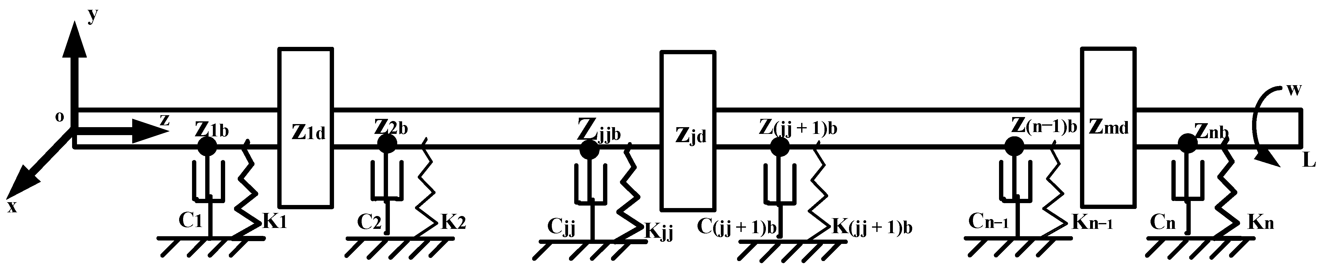
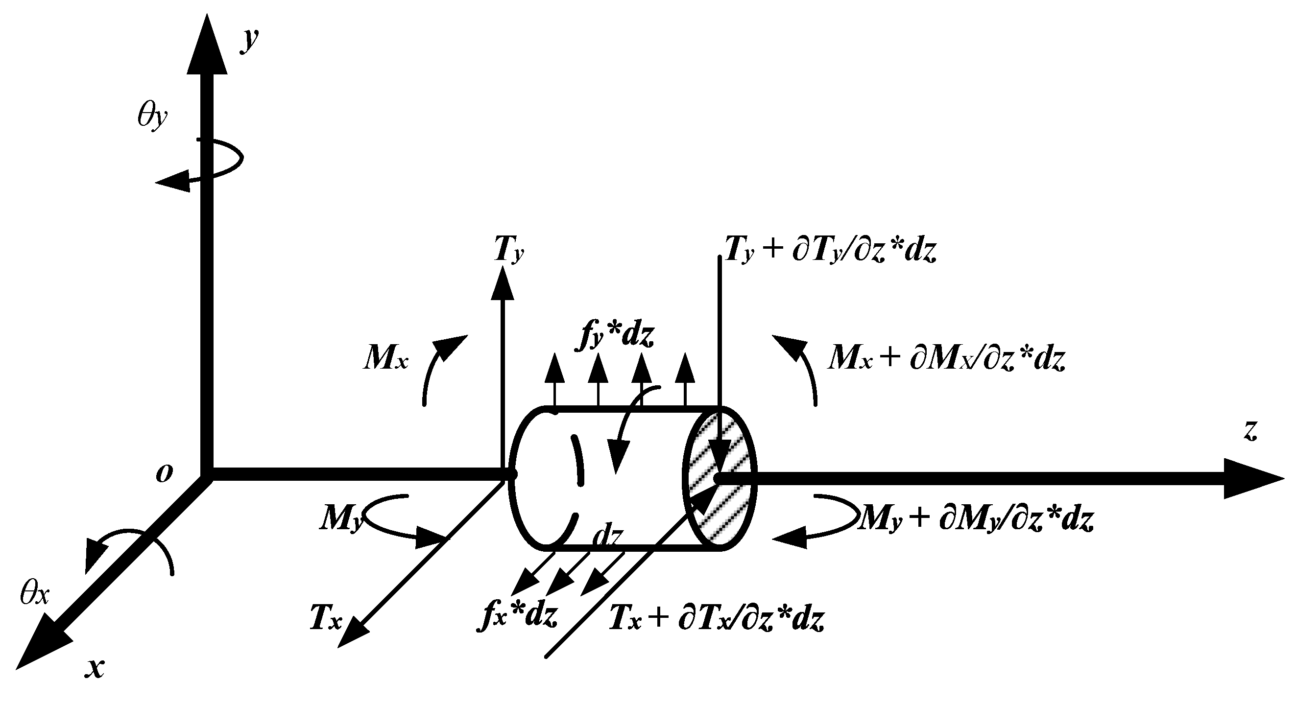
2.1. Continous Model Based on Rayleigh Model
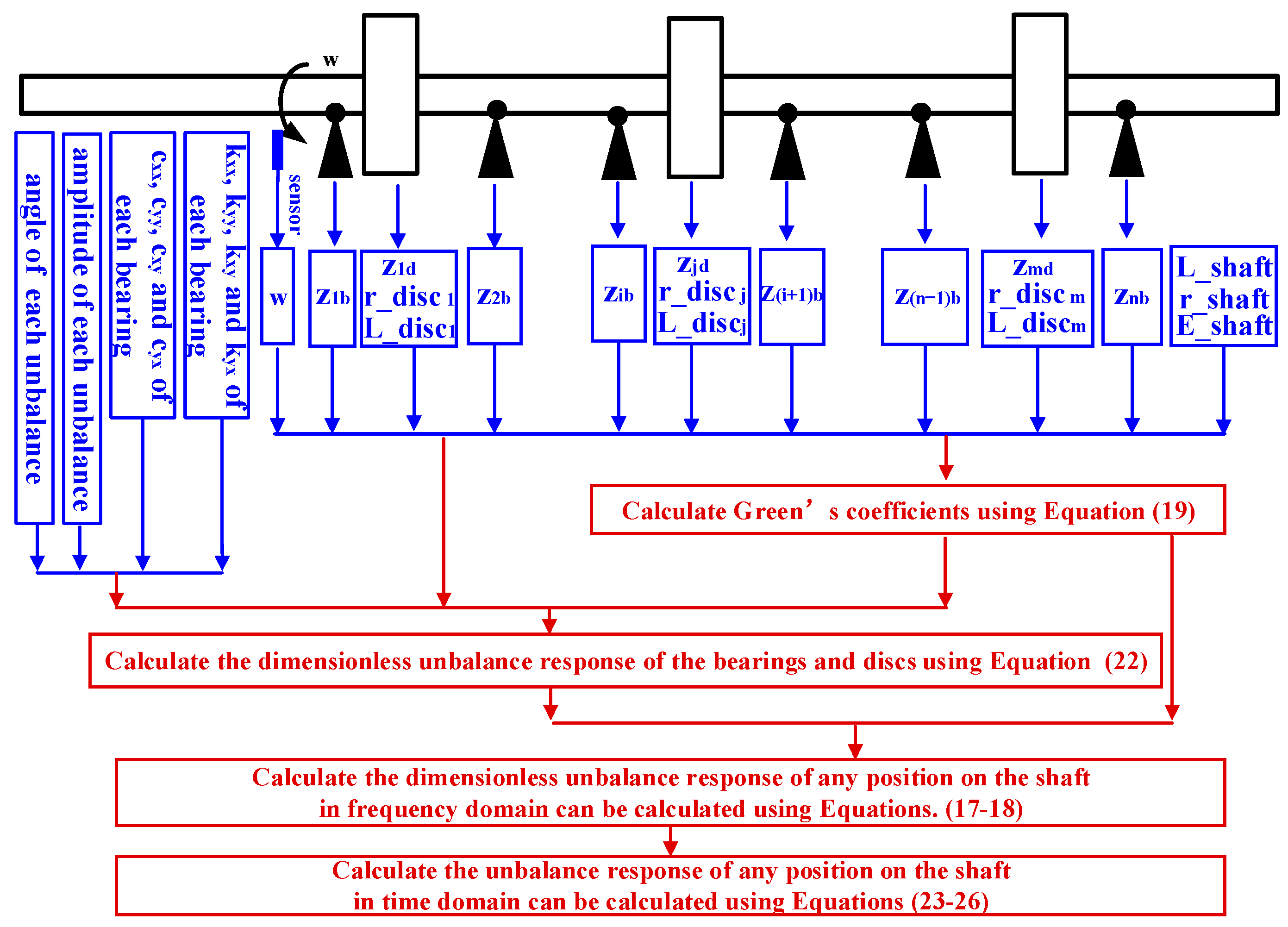
2.2. Analytical Solution
3. Numerical Simulations and Discussion
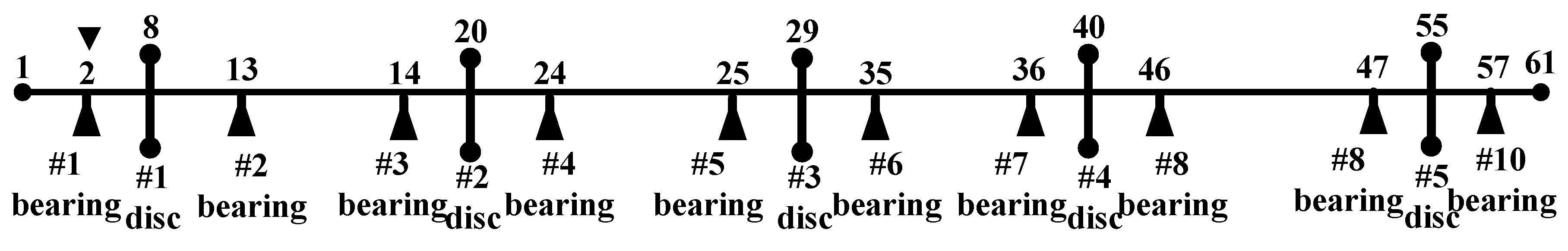
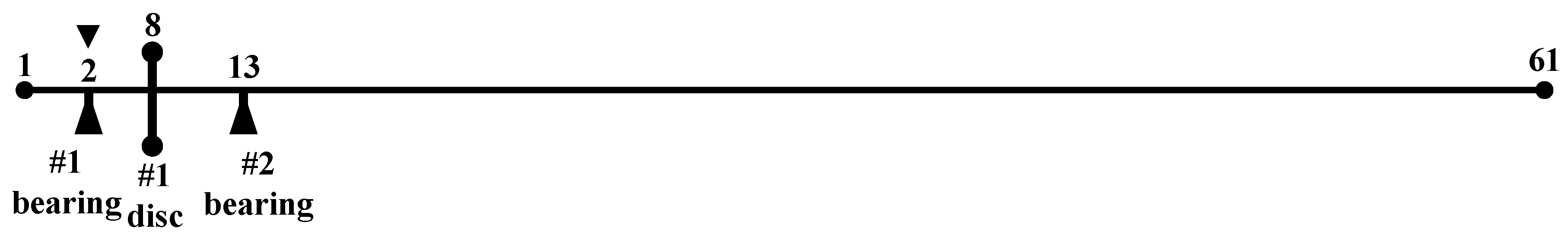
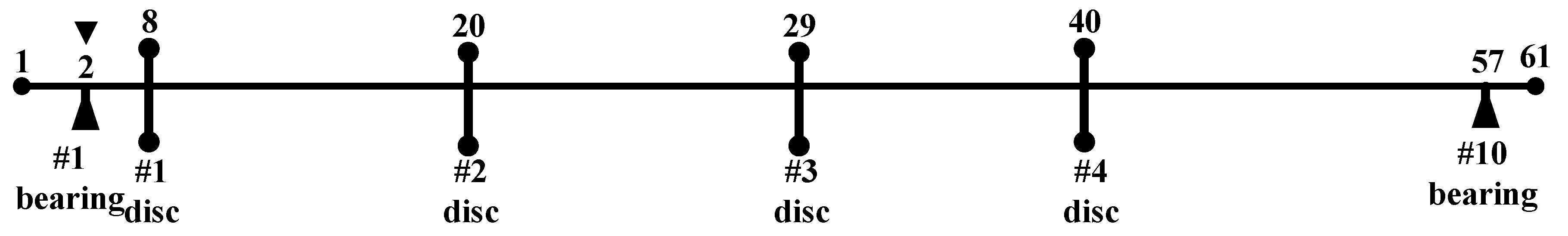
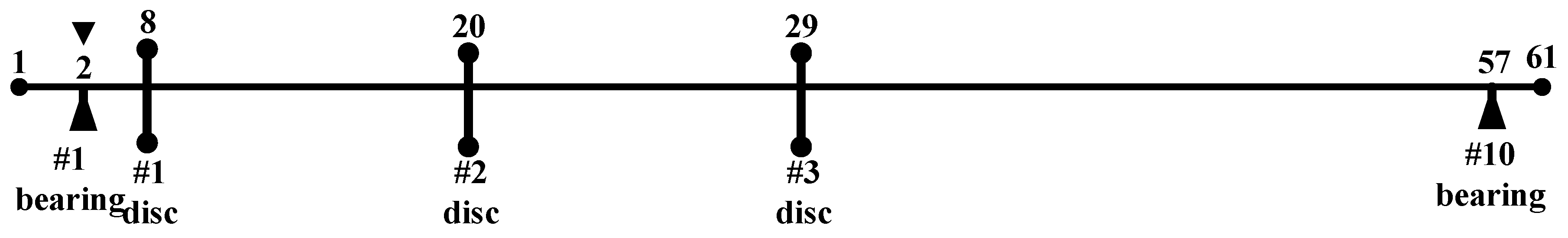
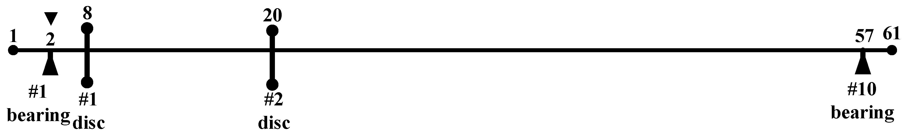
3.1. Methodology of Numerical Simulations
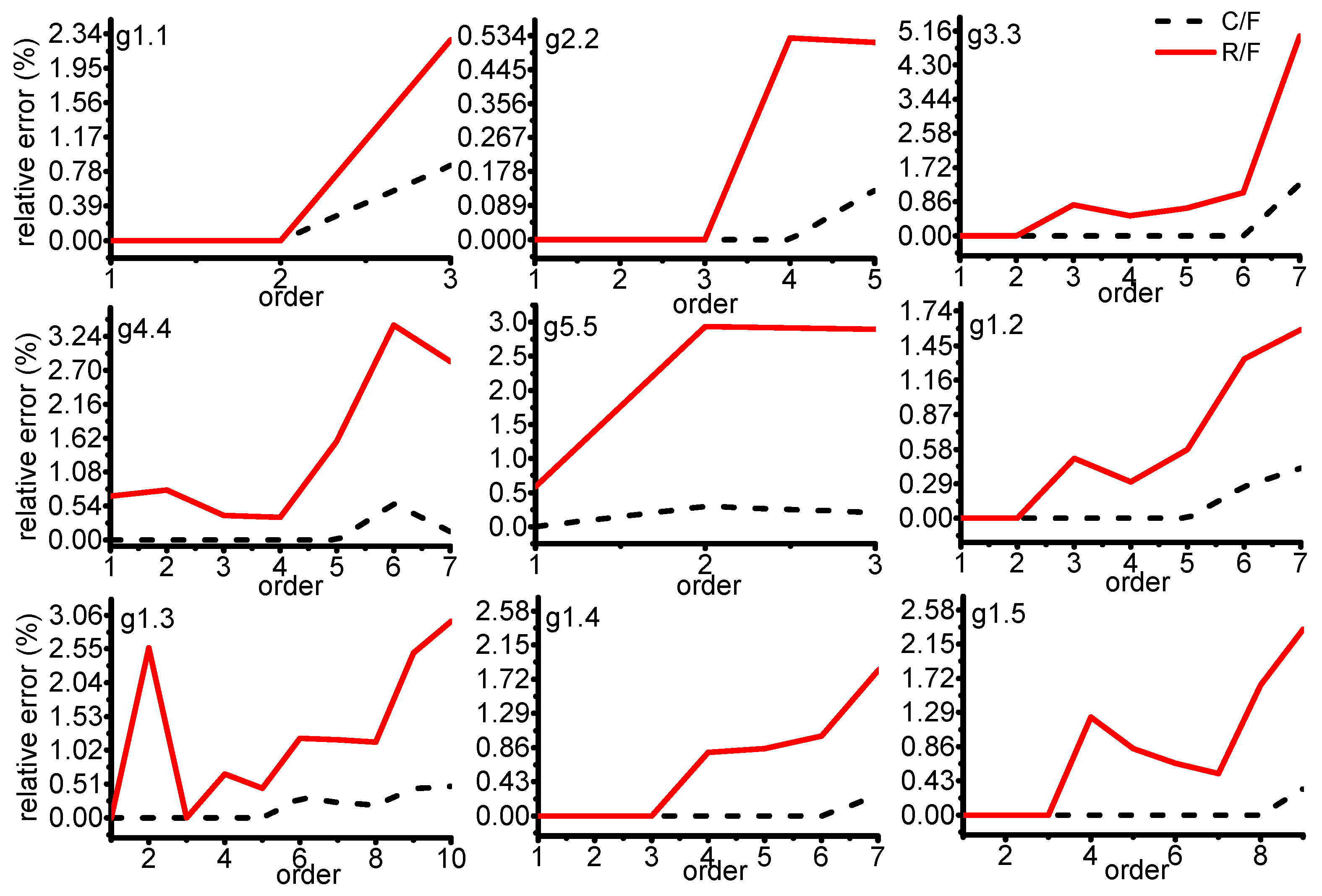
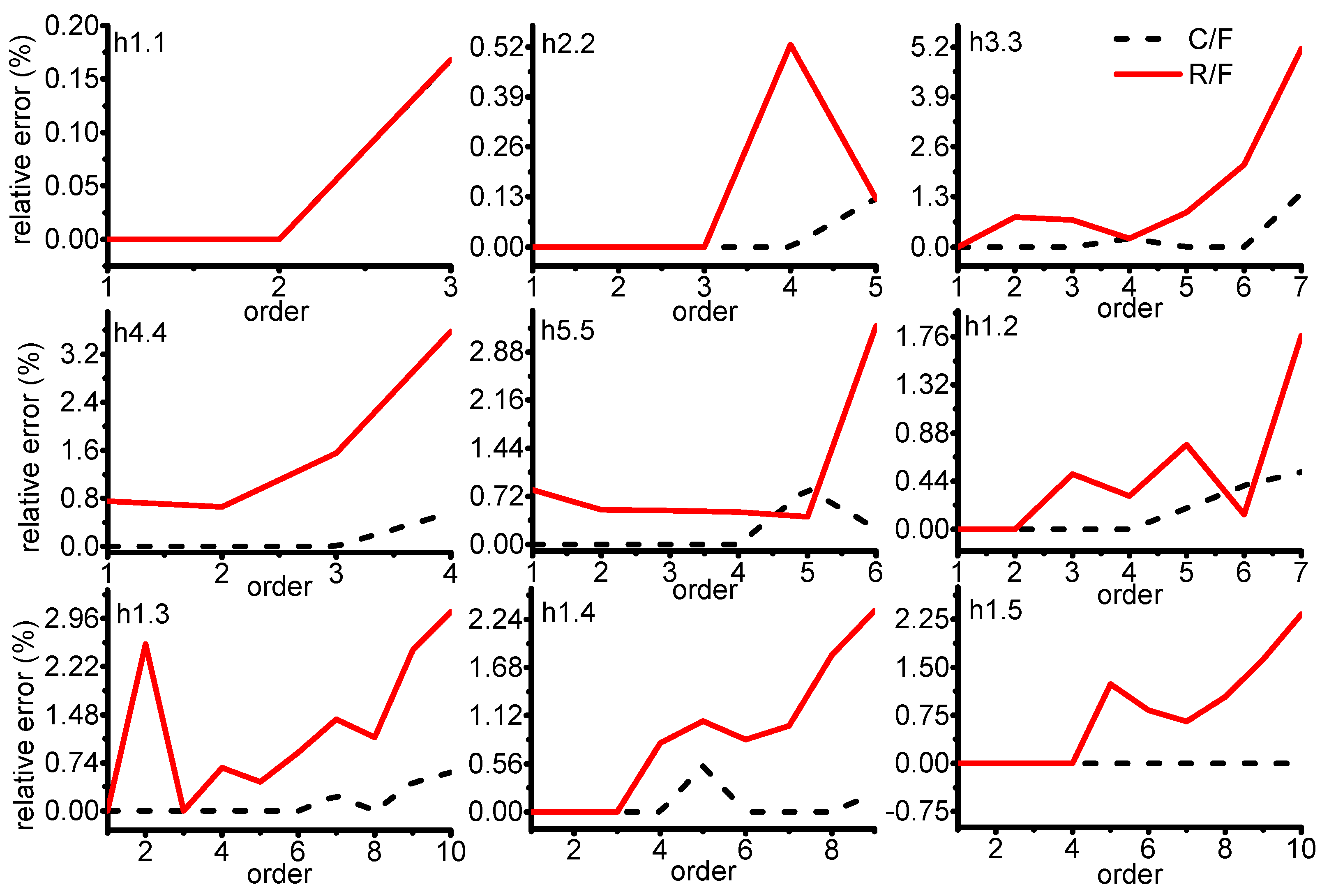
3.2. Calculated Critical Frequencies
3.2.1. Results
3.2.2. Discussion
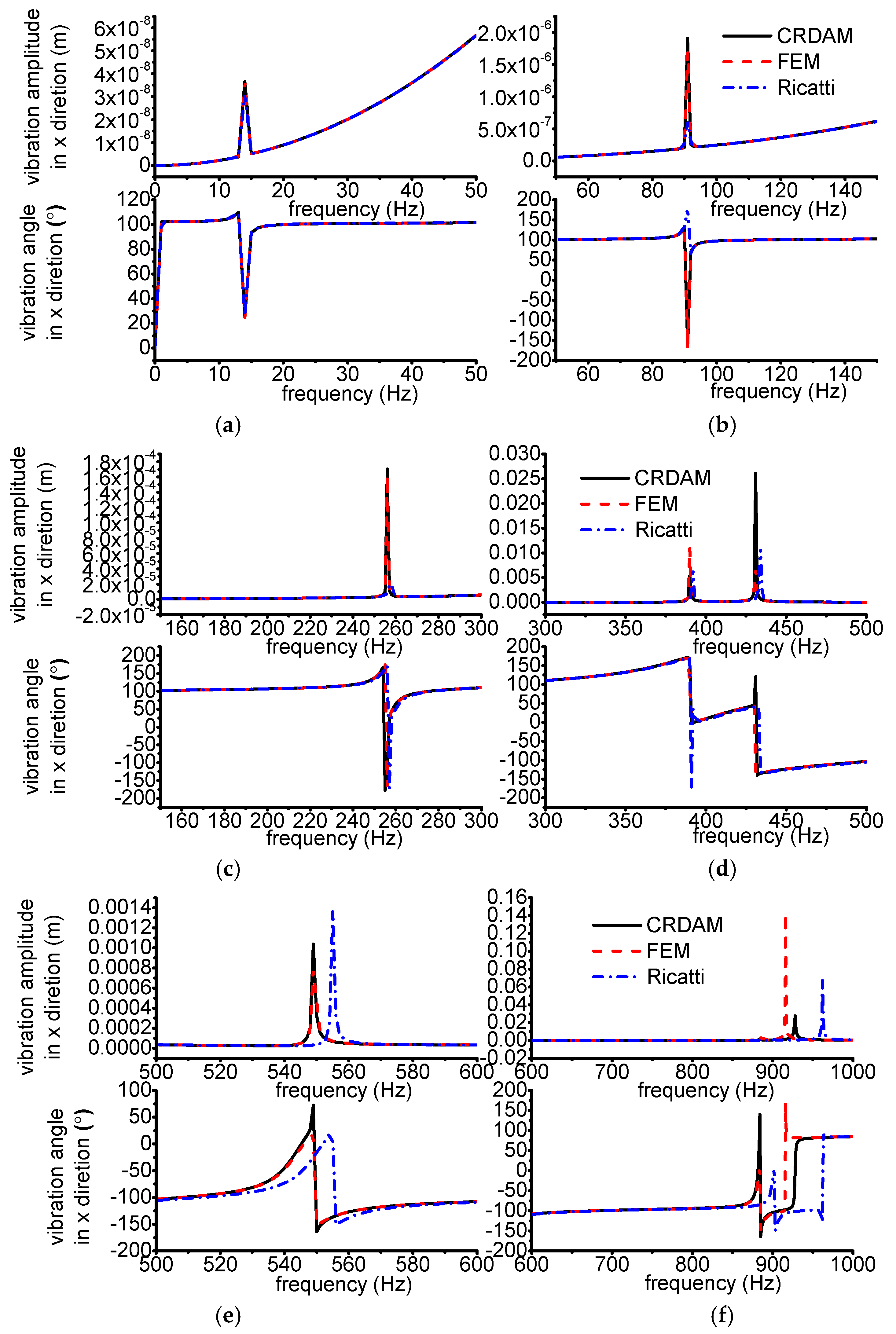
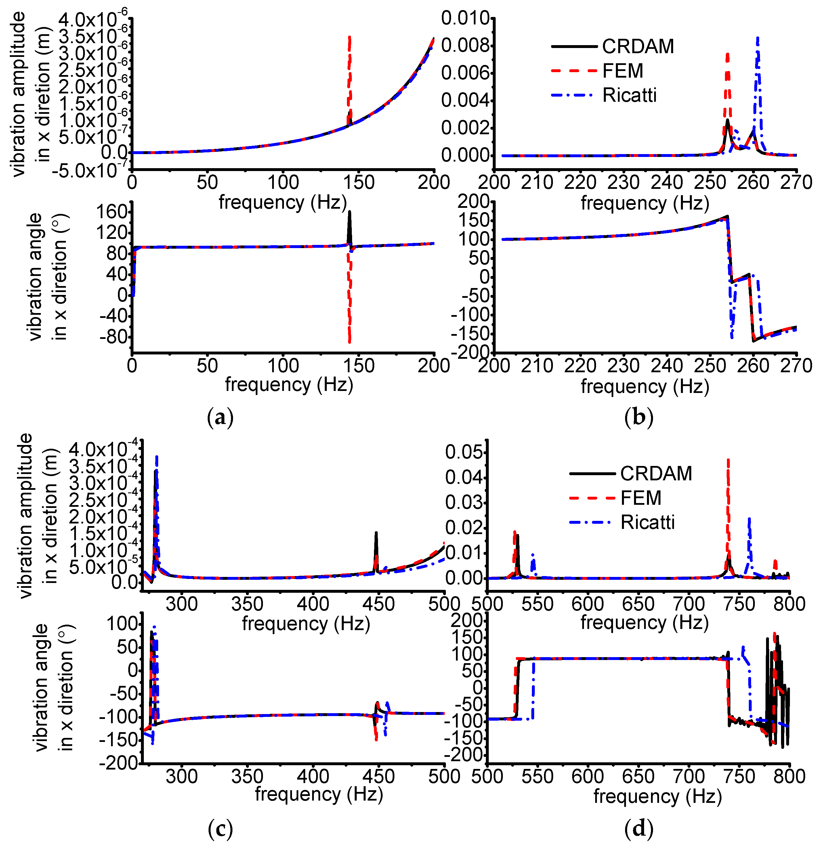
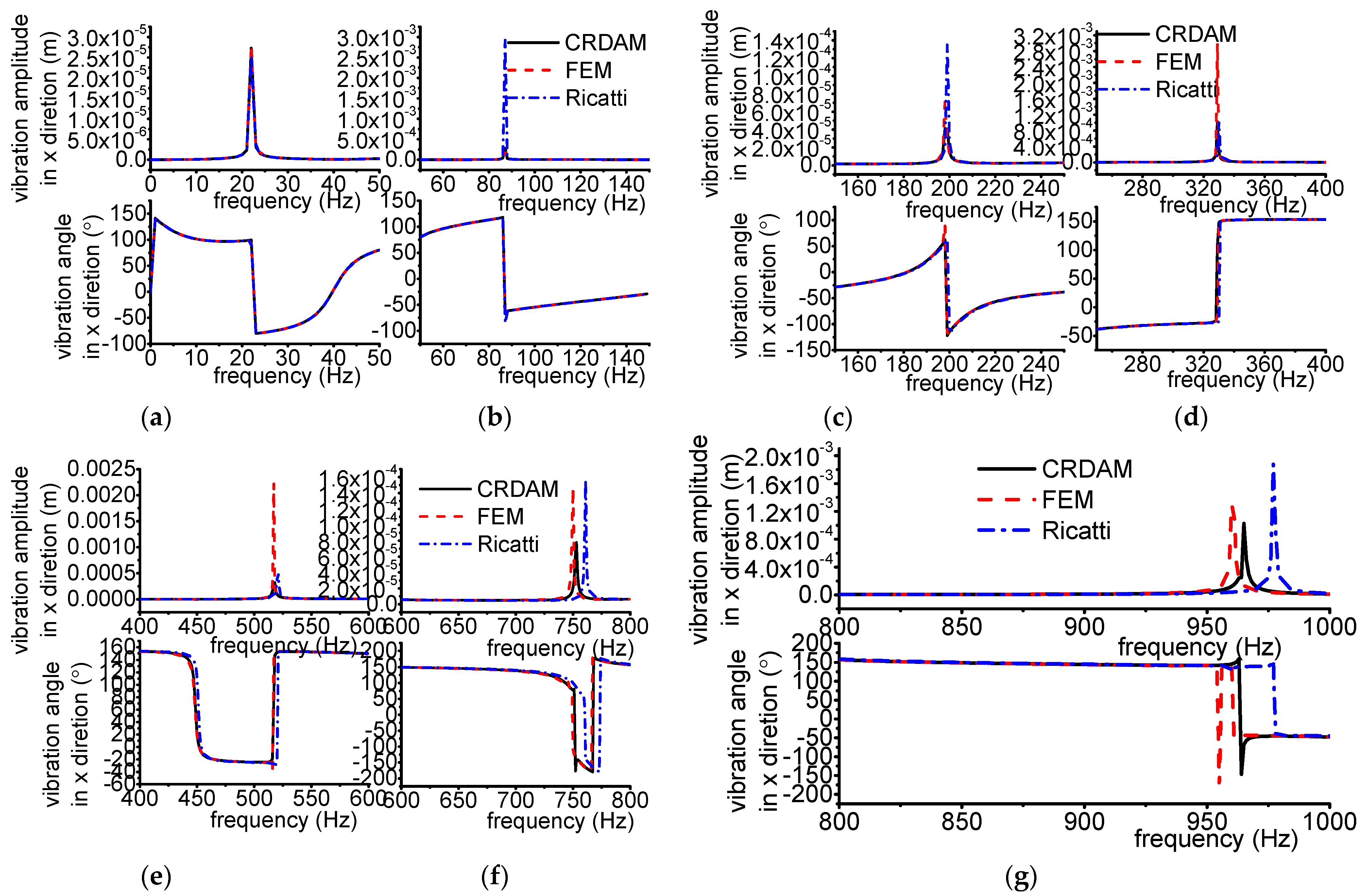
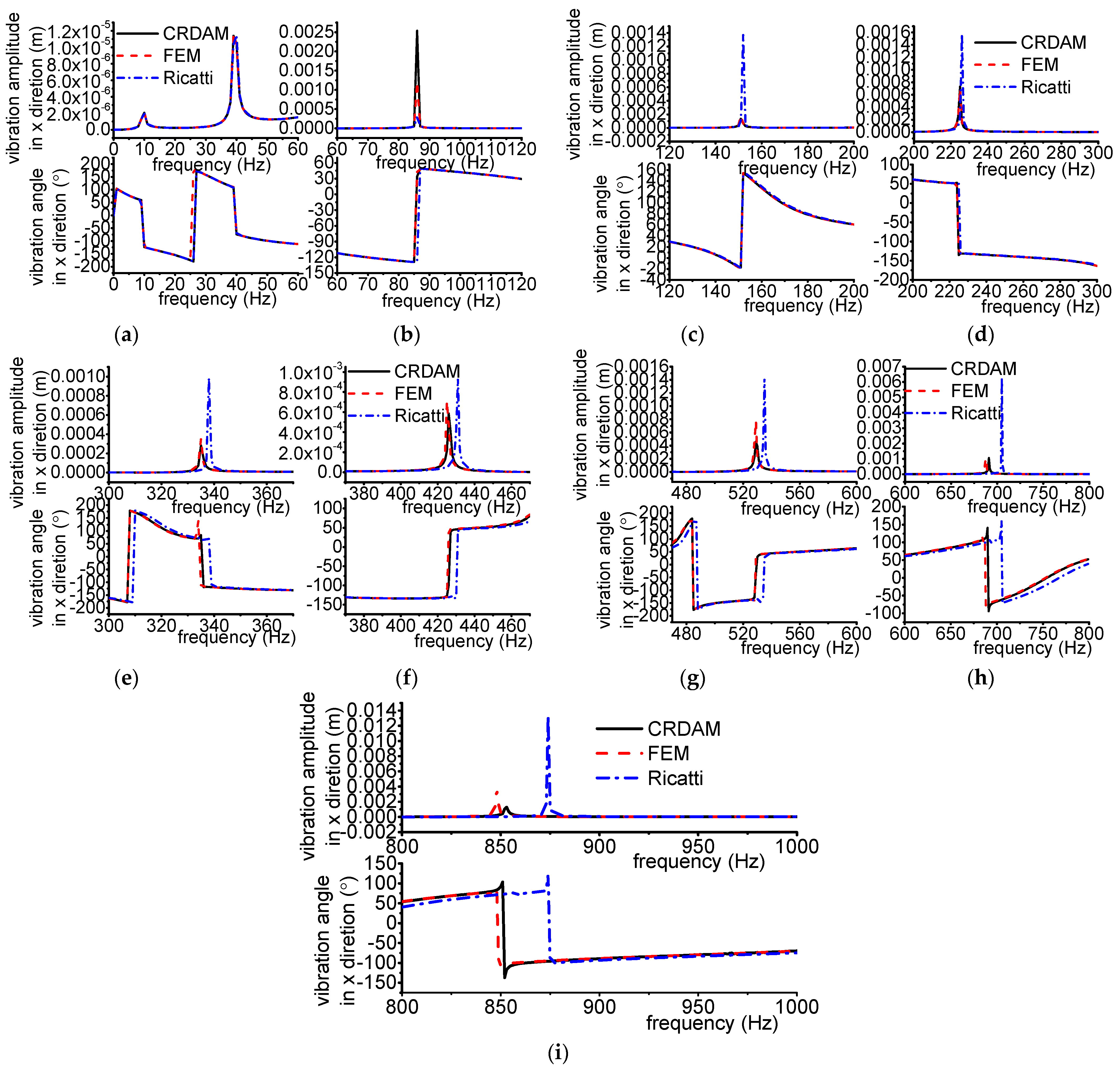
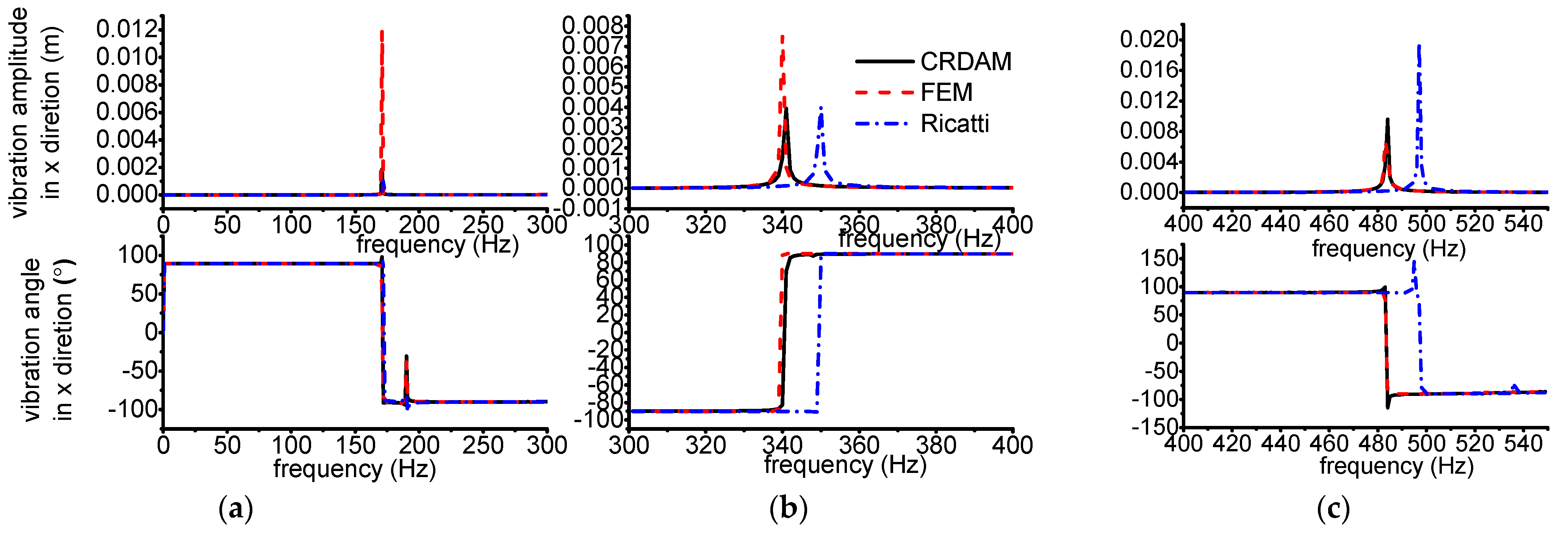
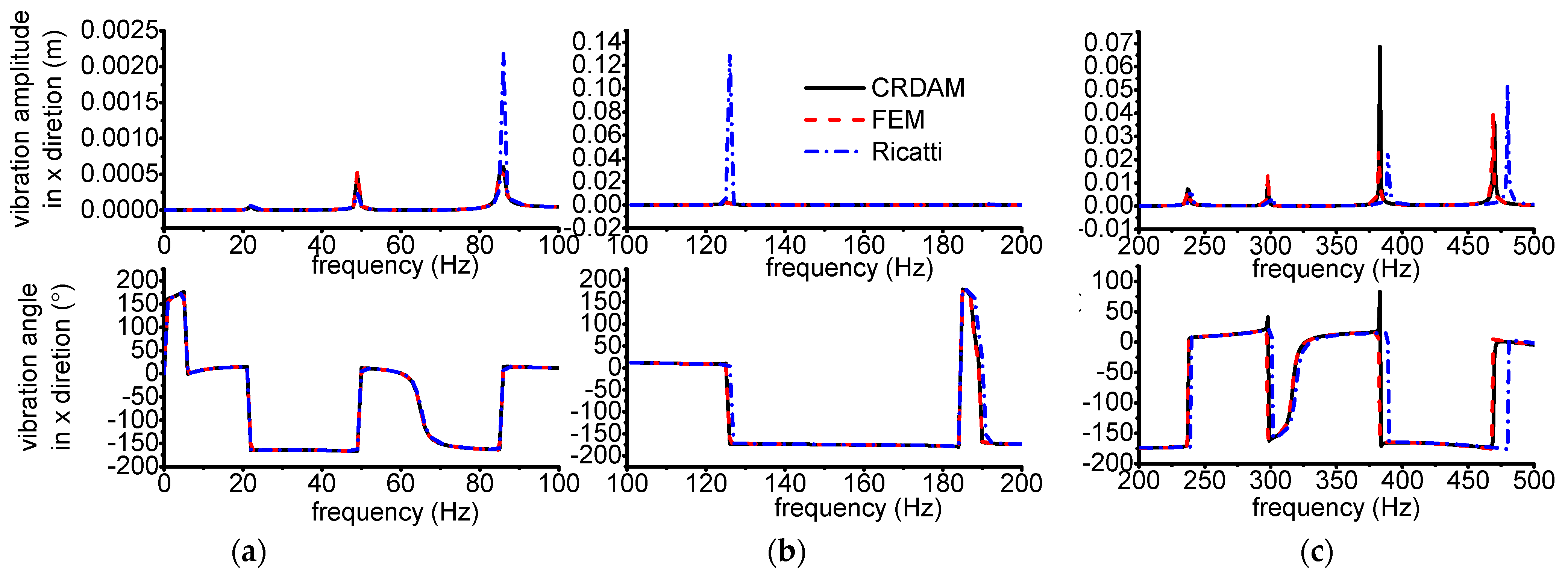
3.3. Calculated Unbalance Response
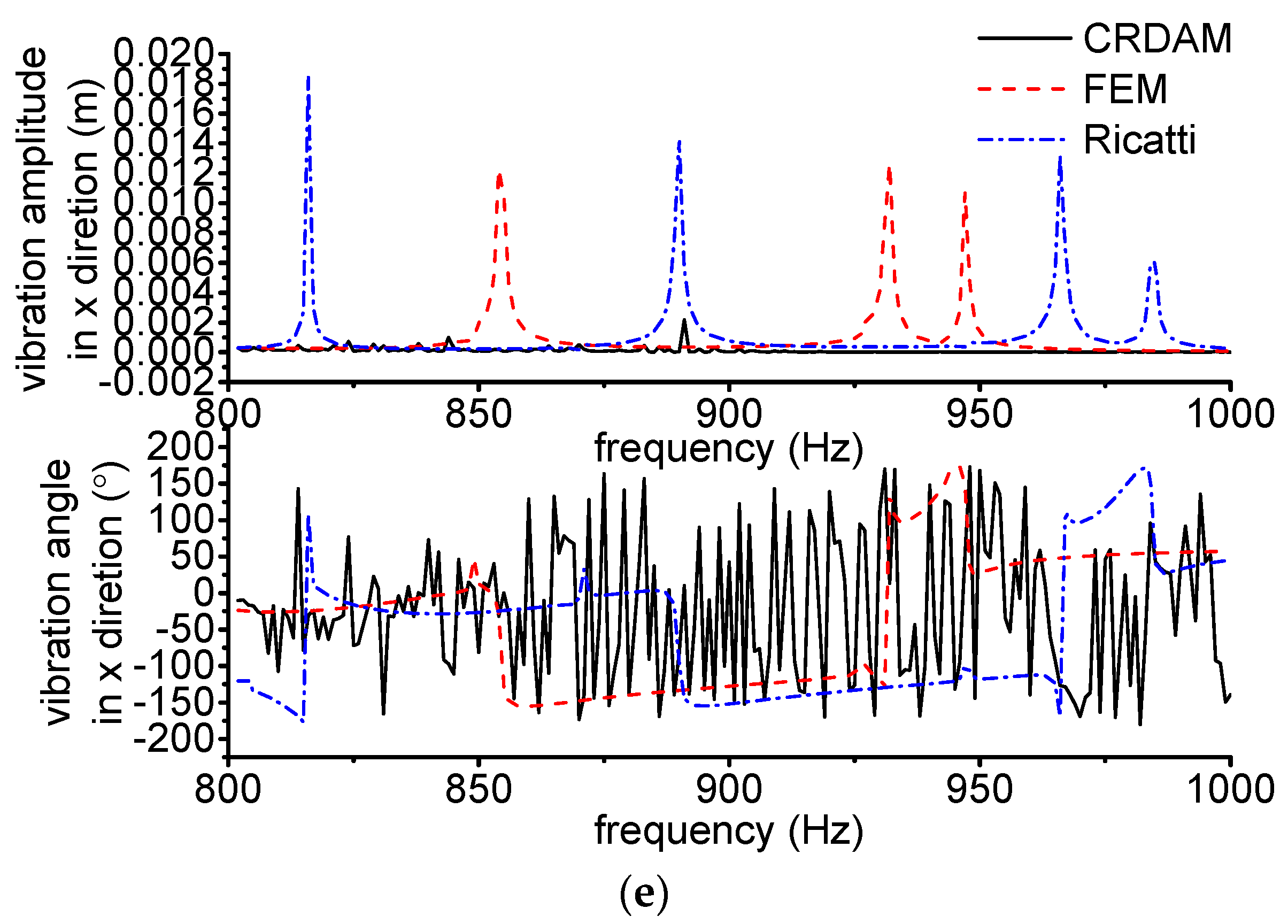
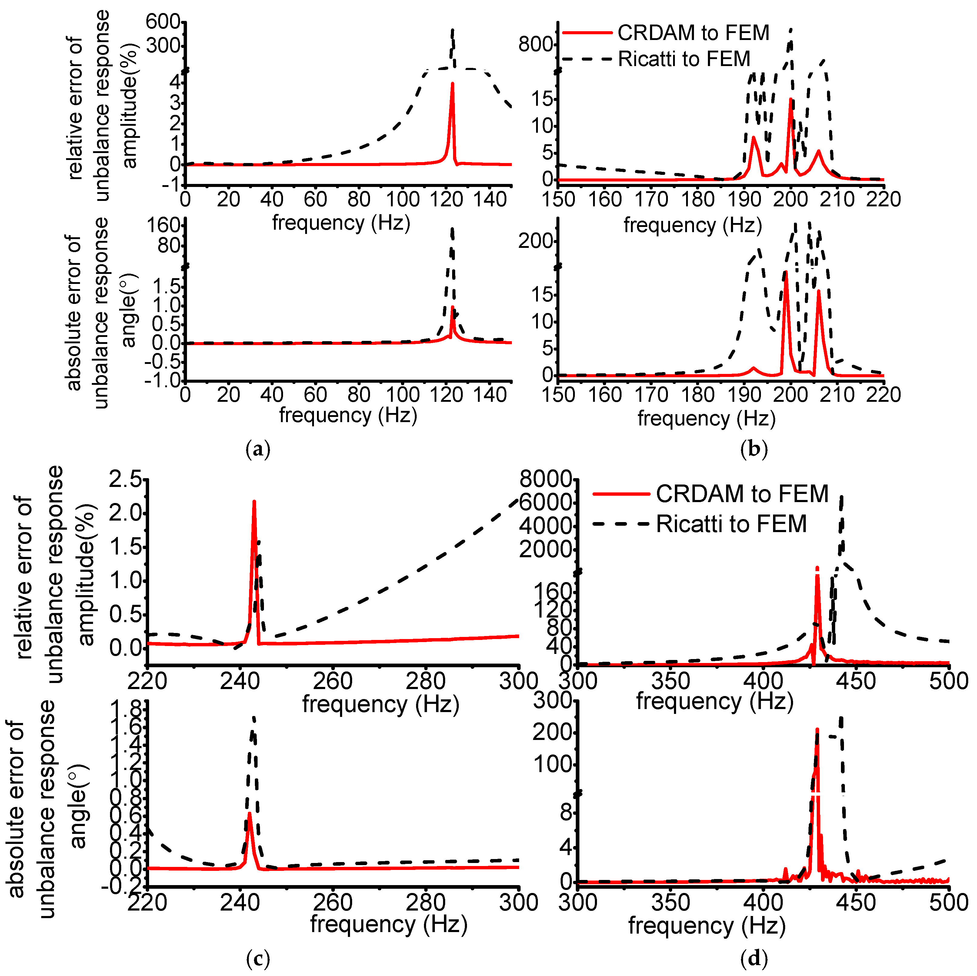
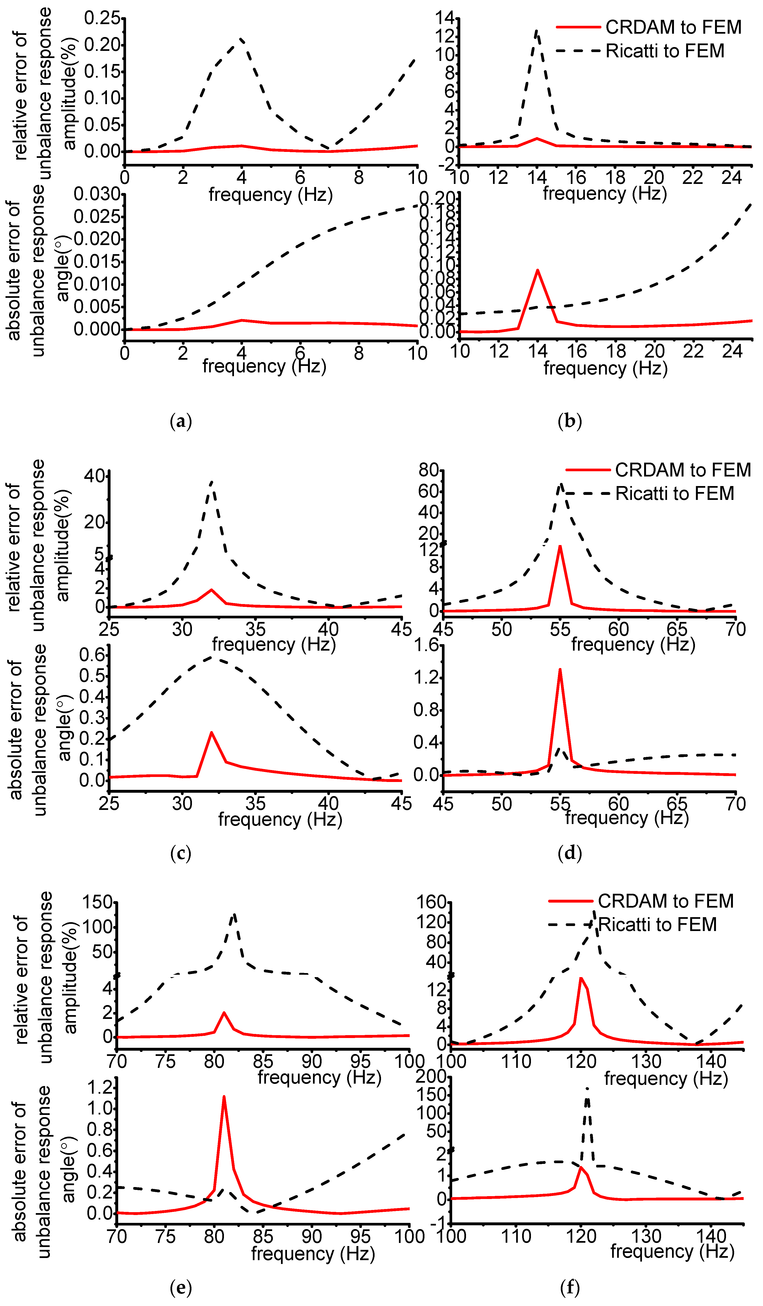
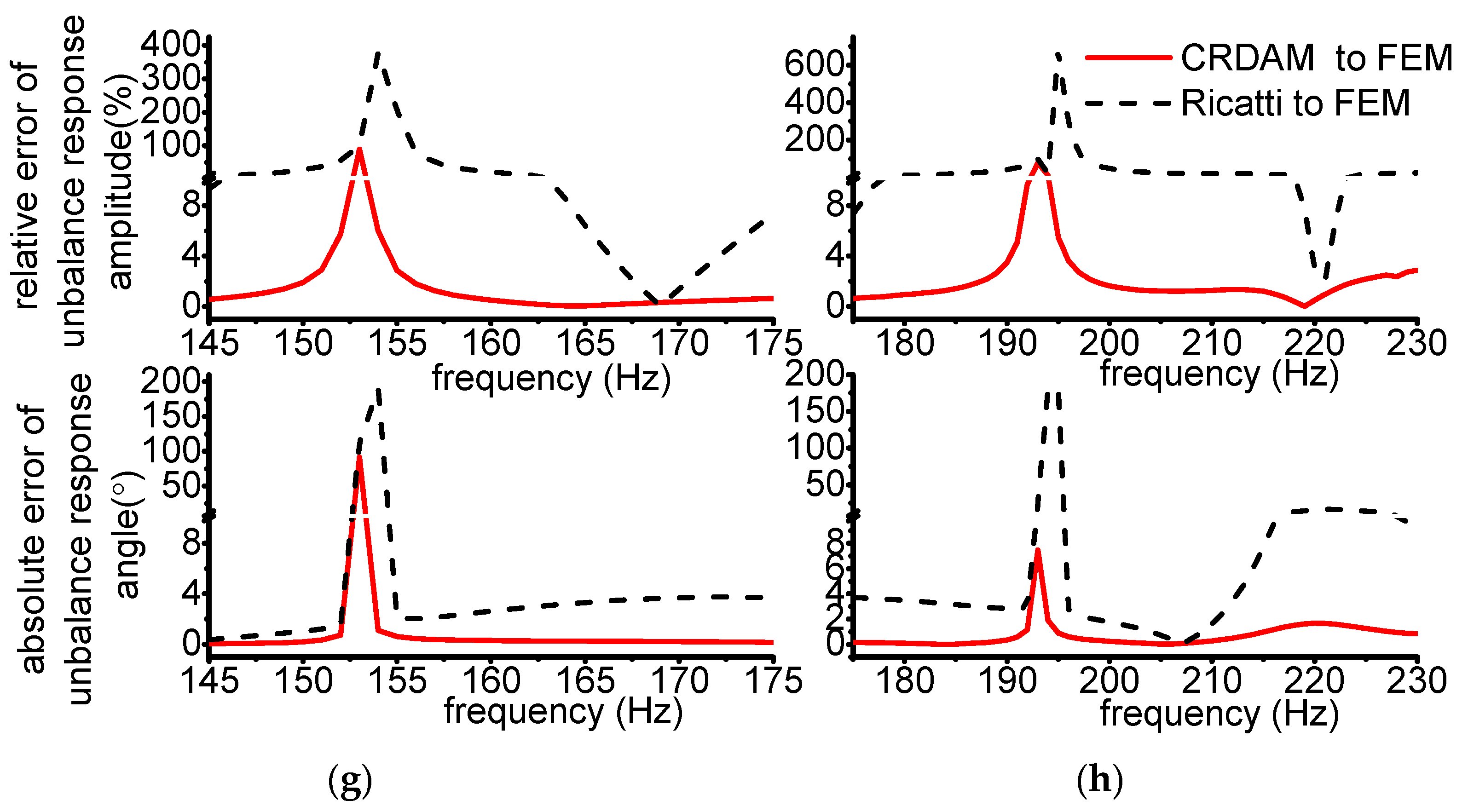
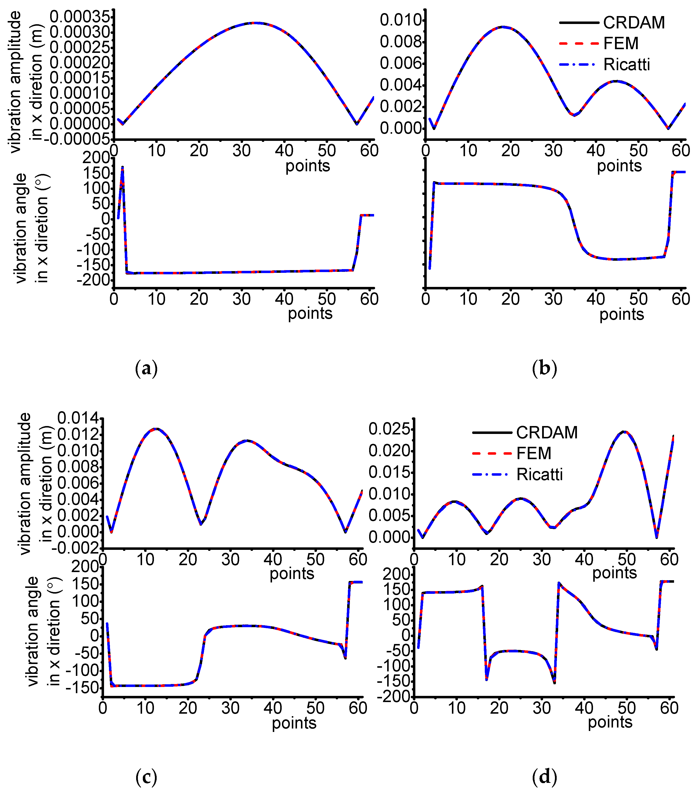
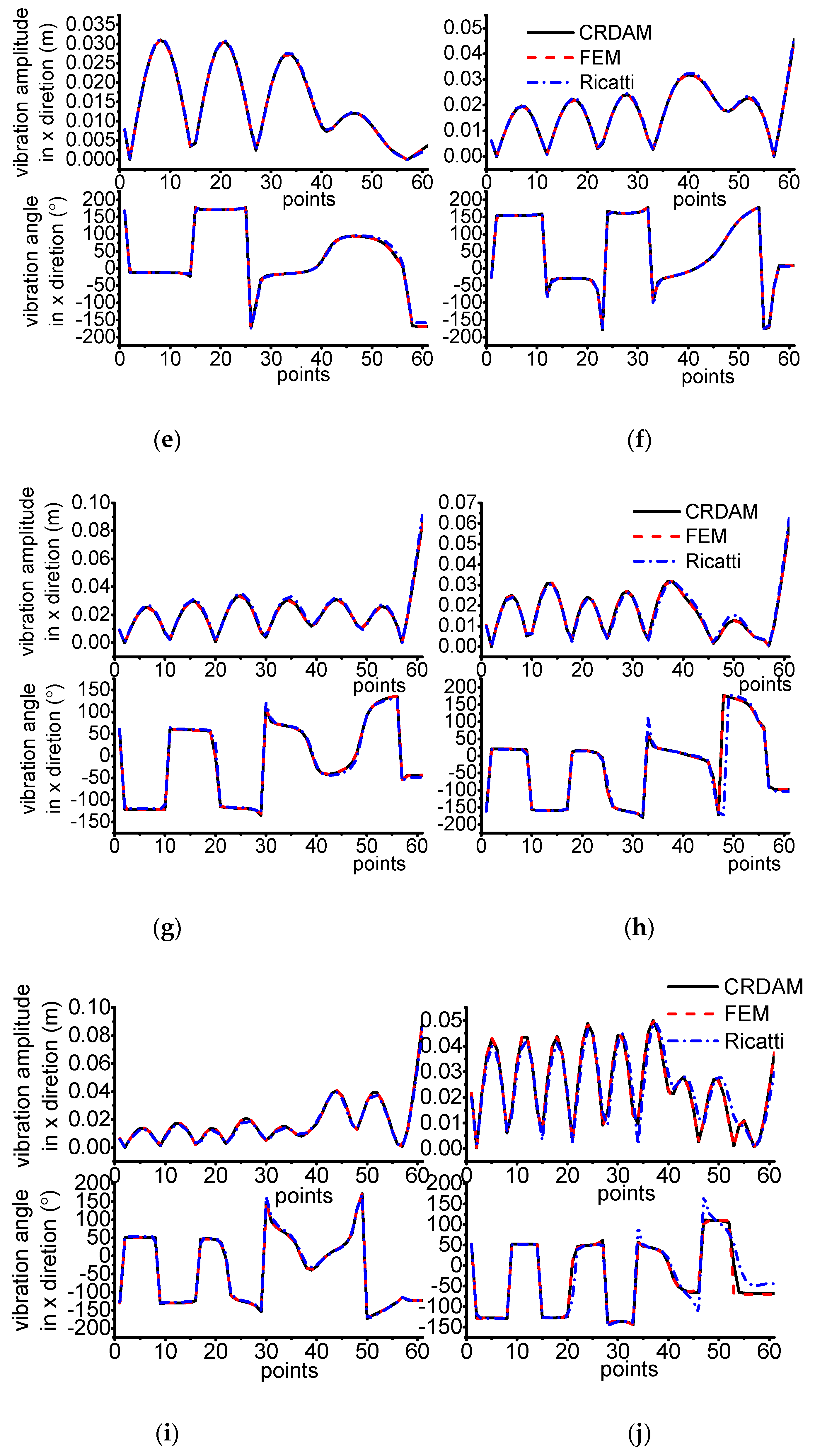
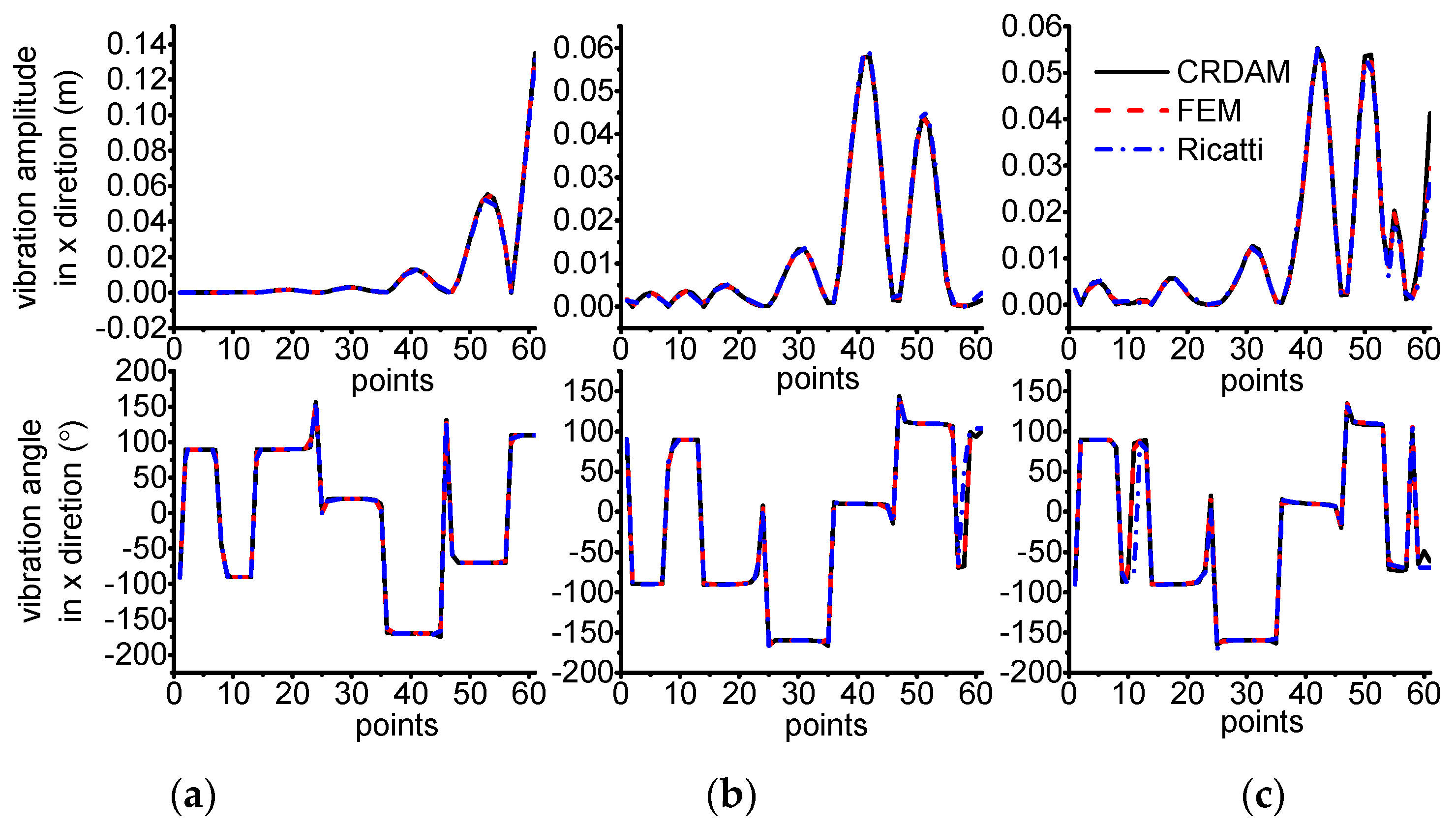
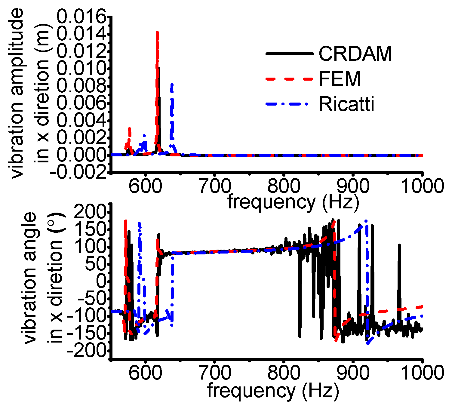
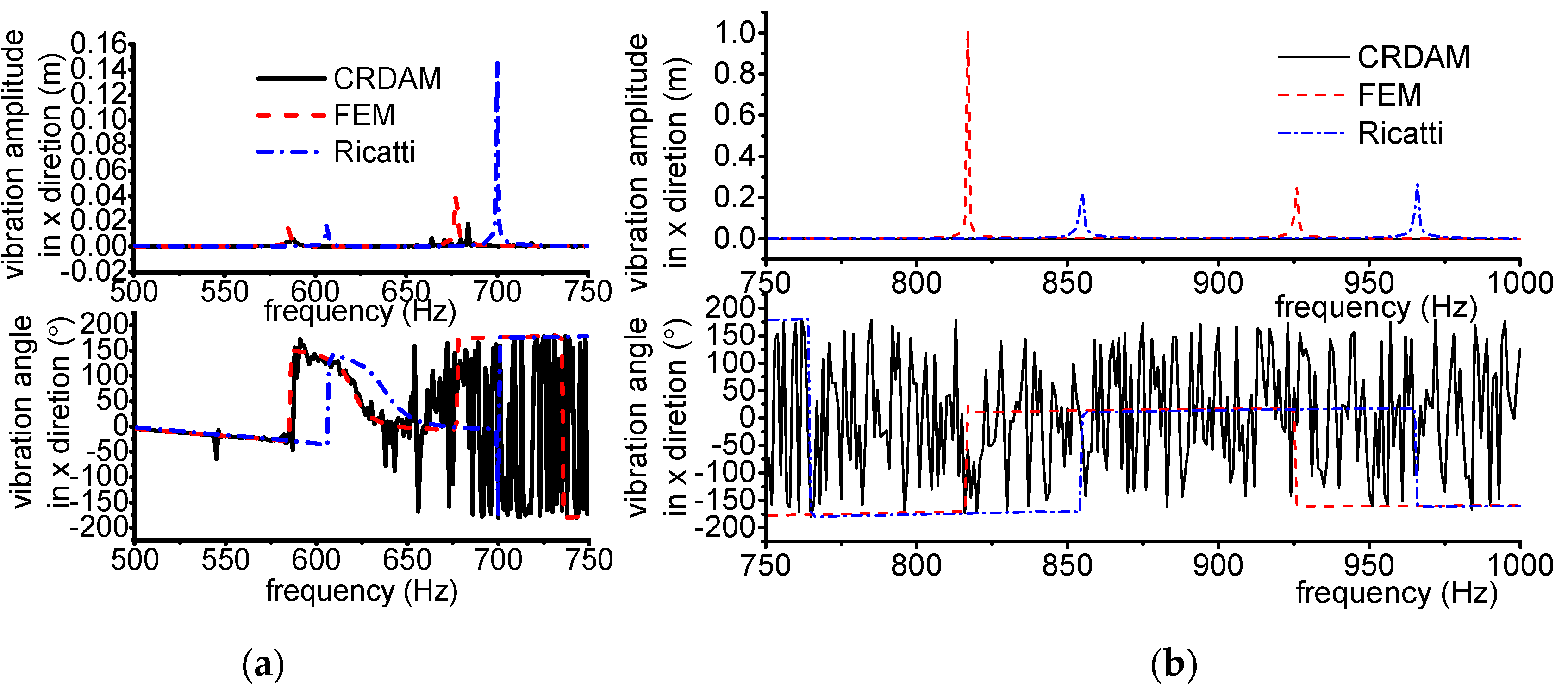
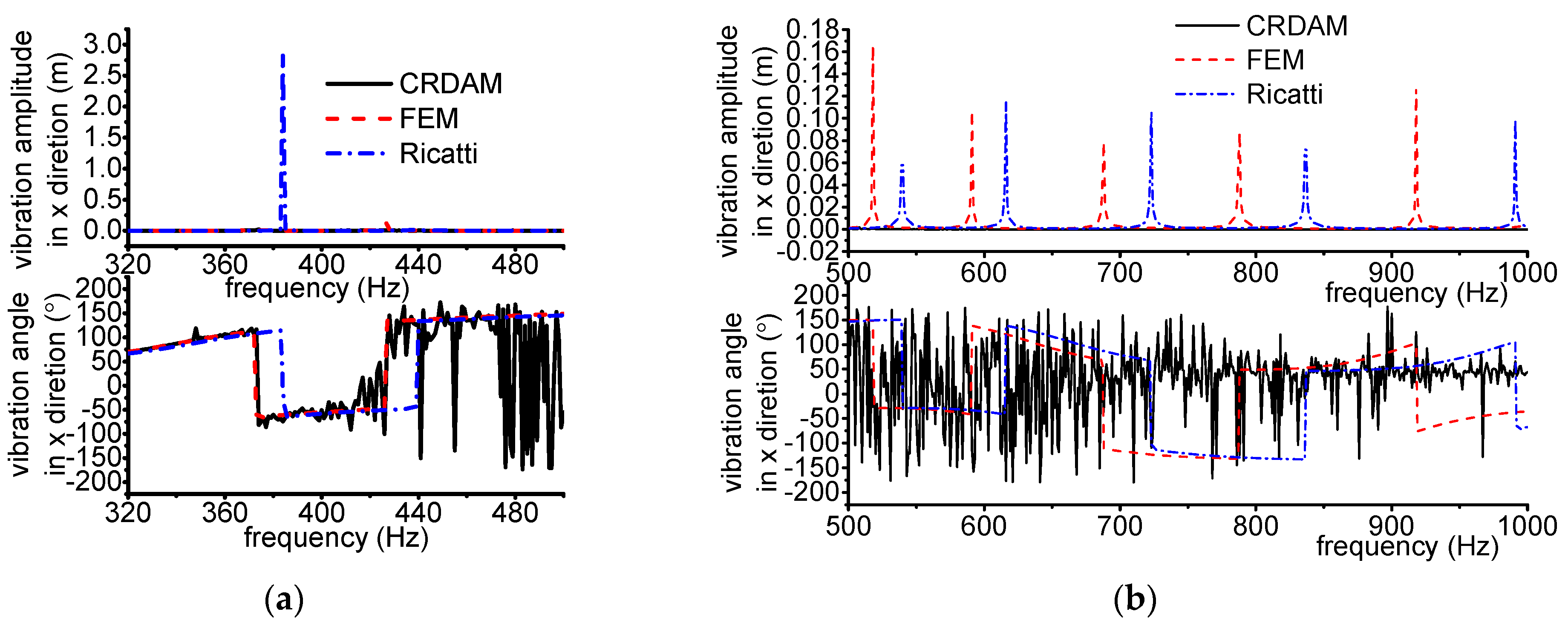
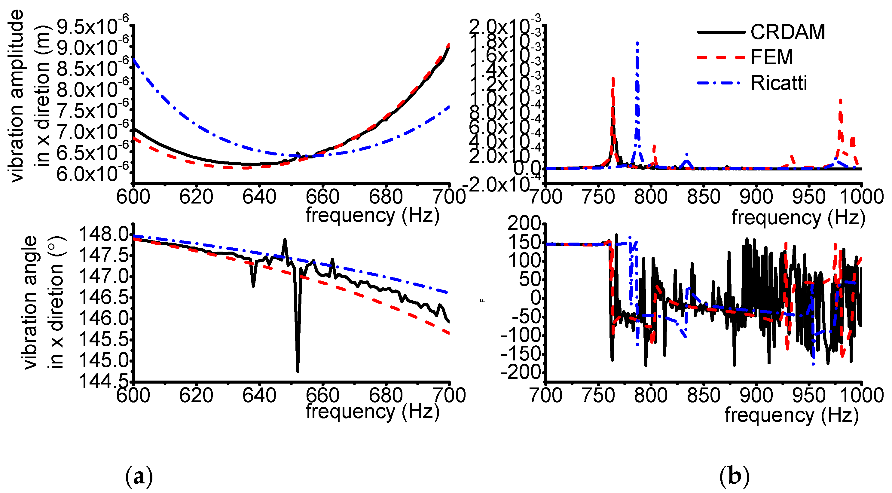
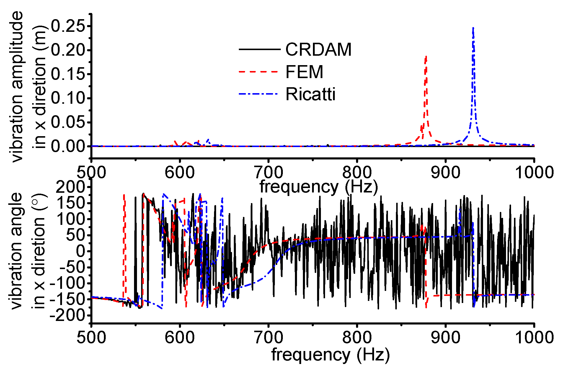
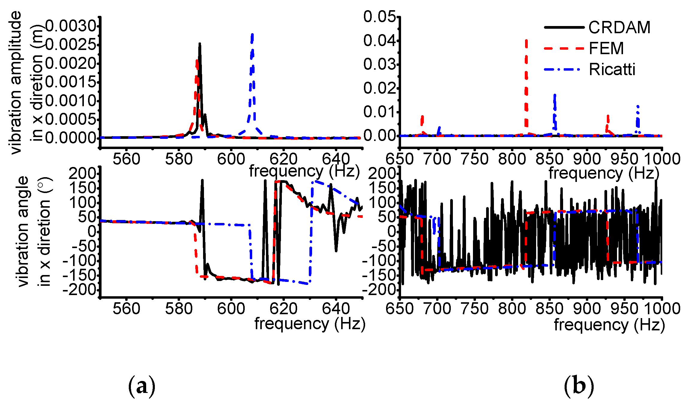
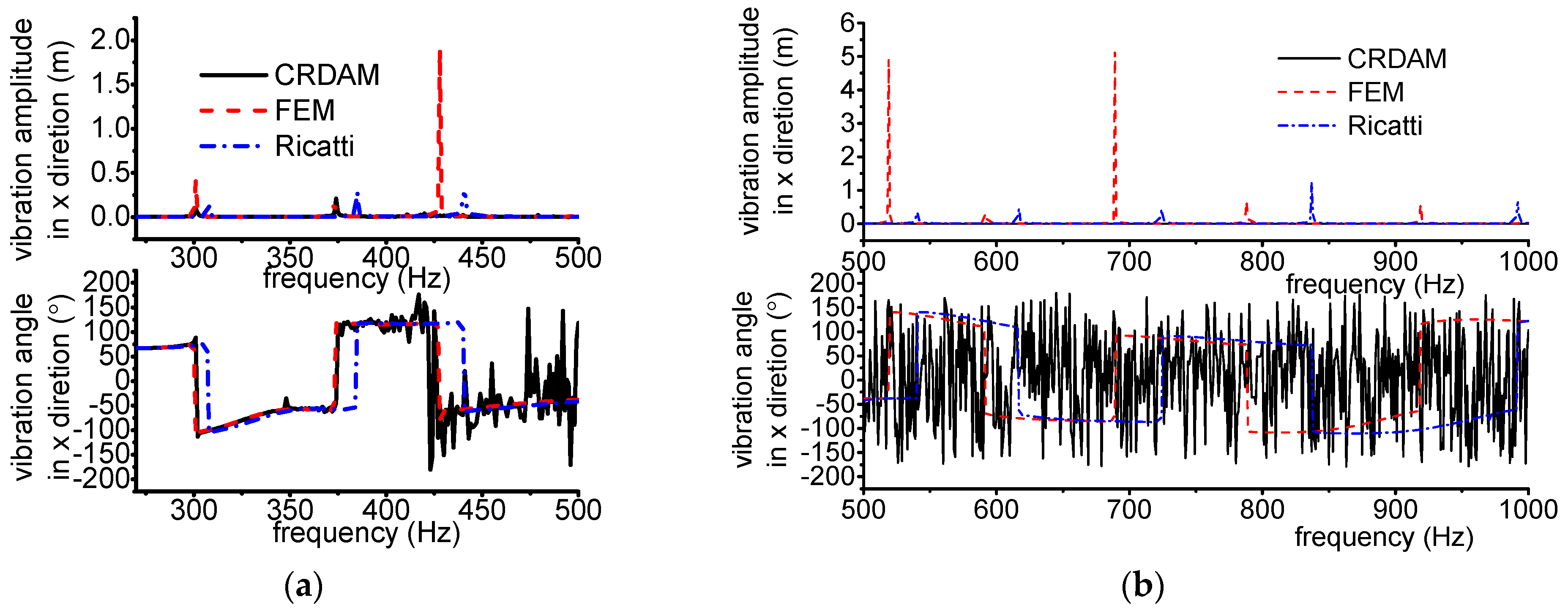
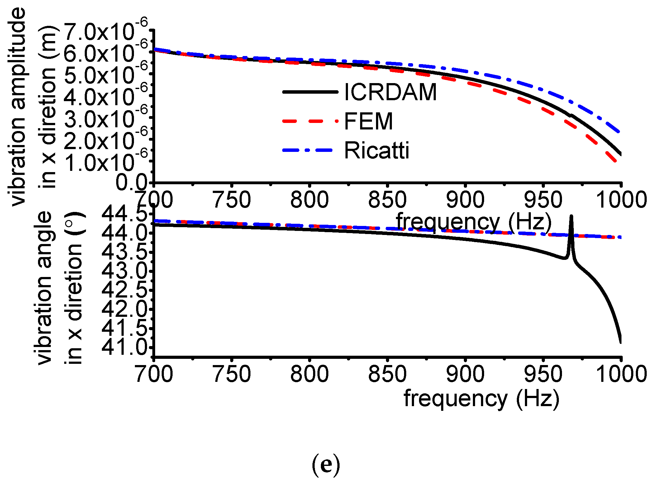
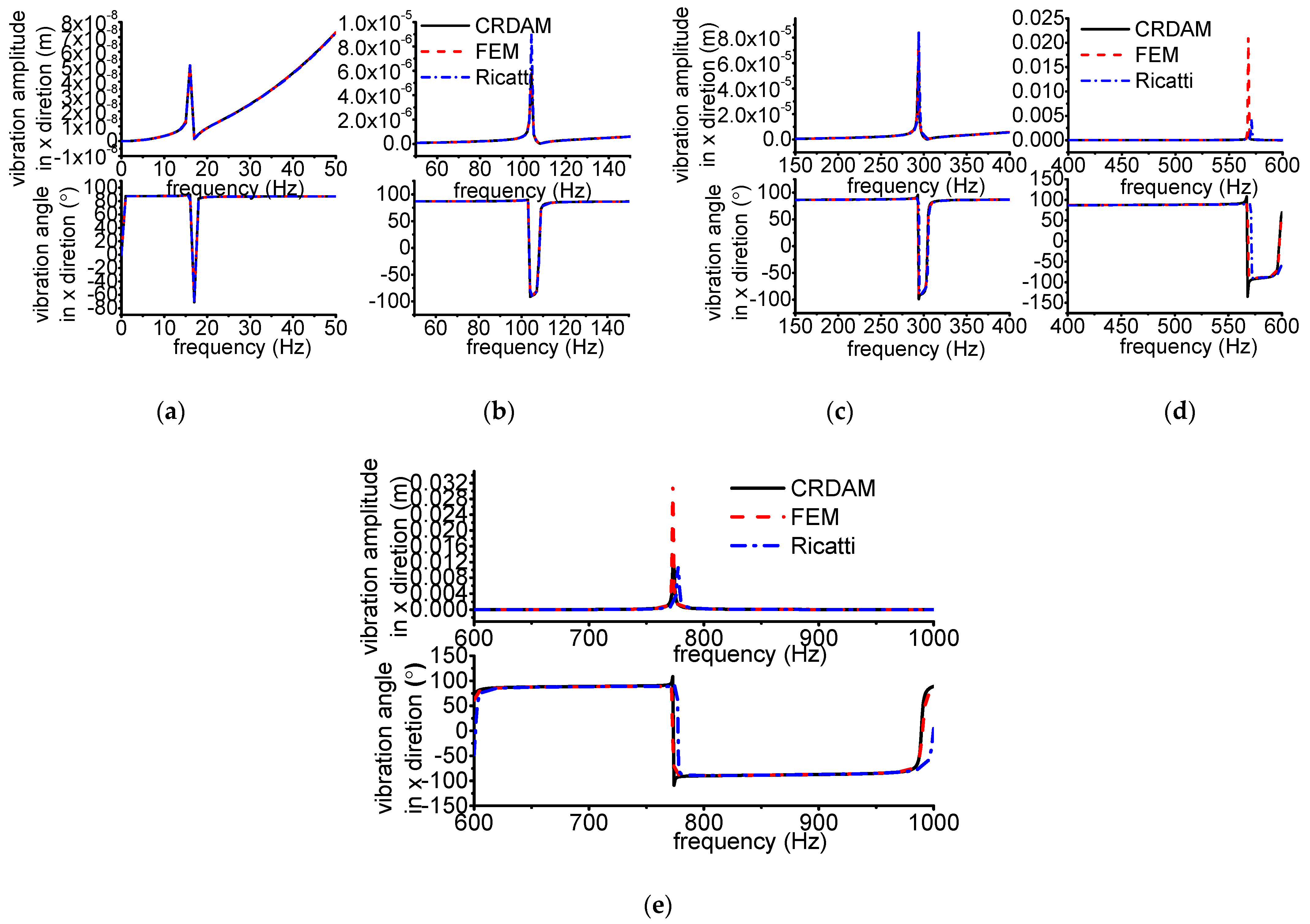
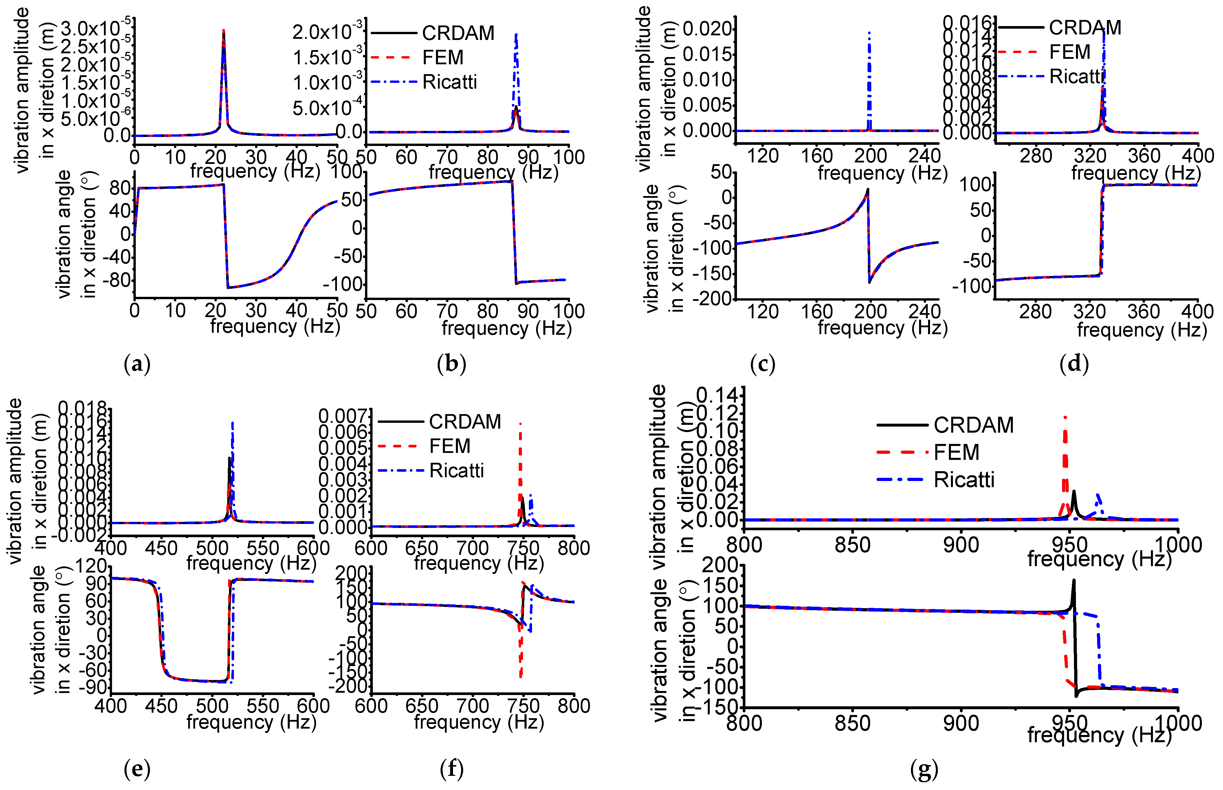
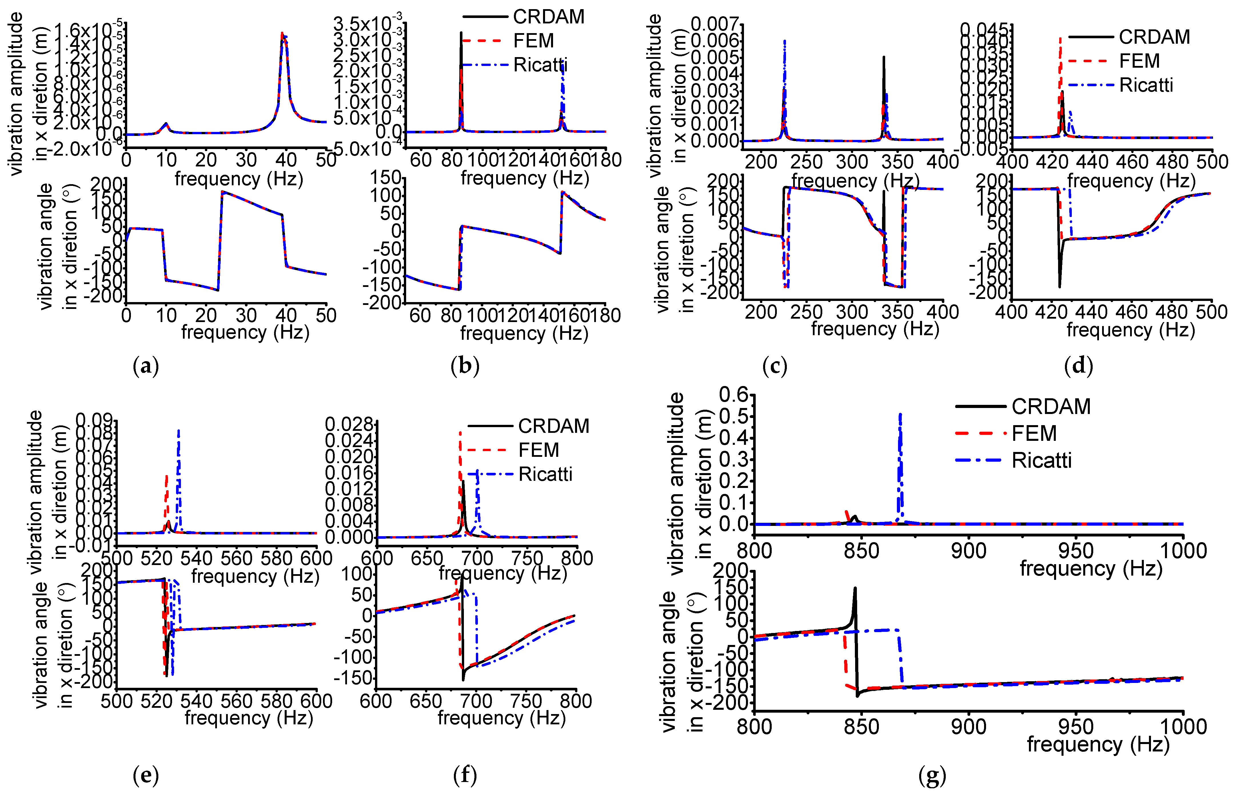
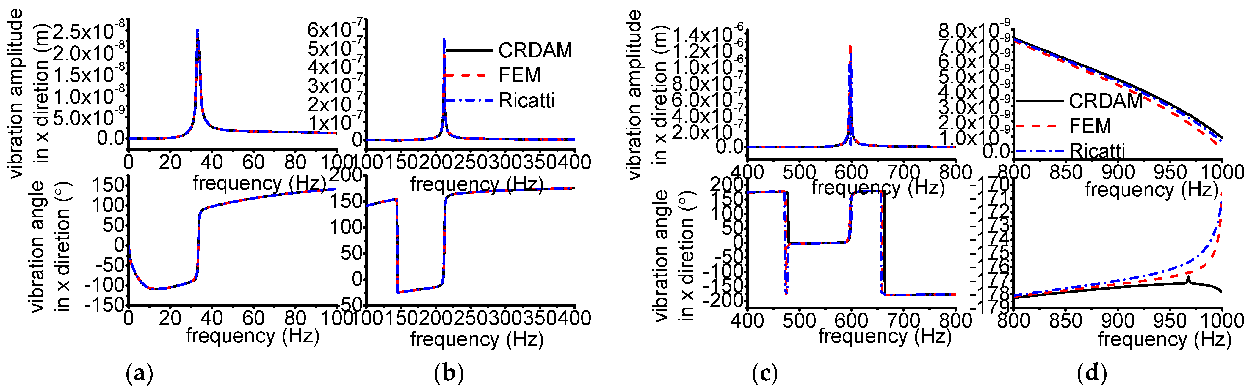
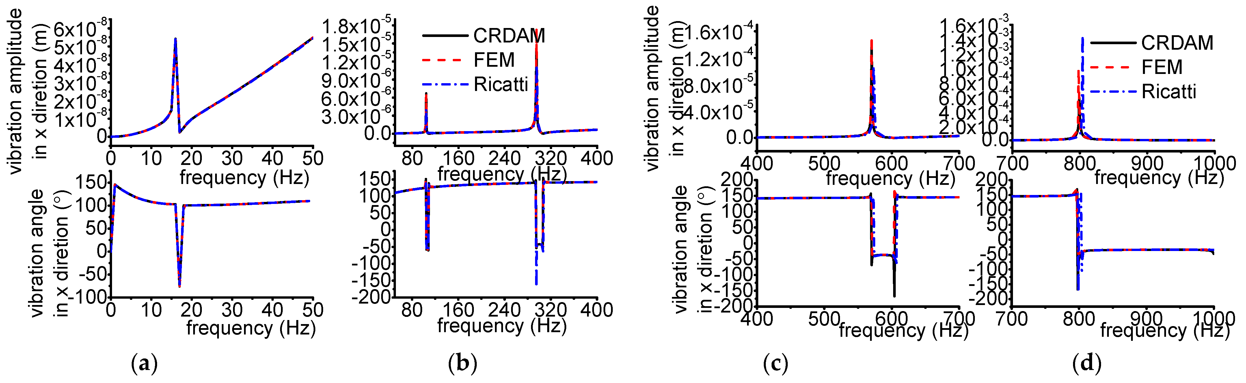
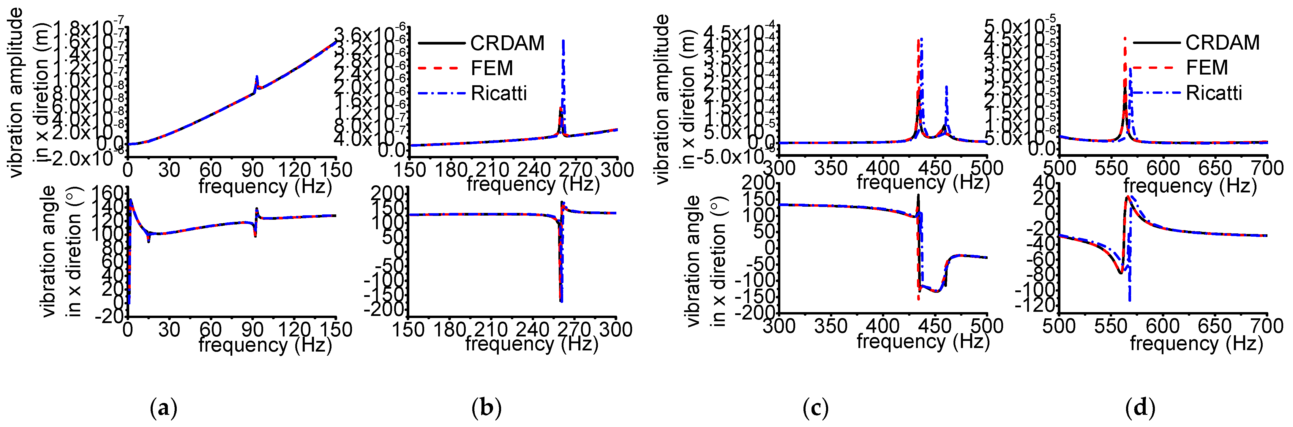
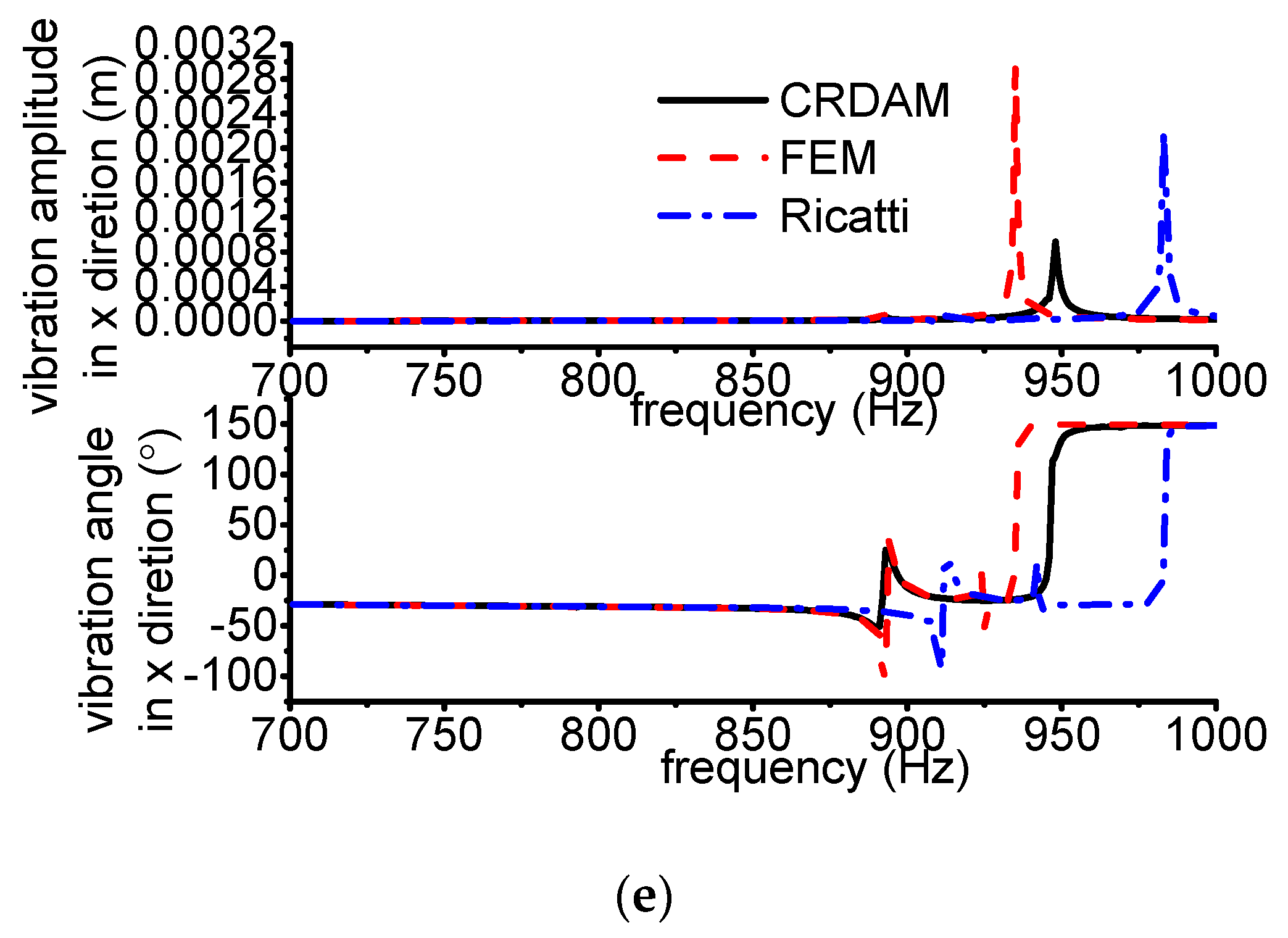
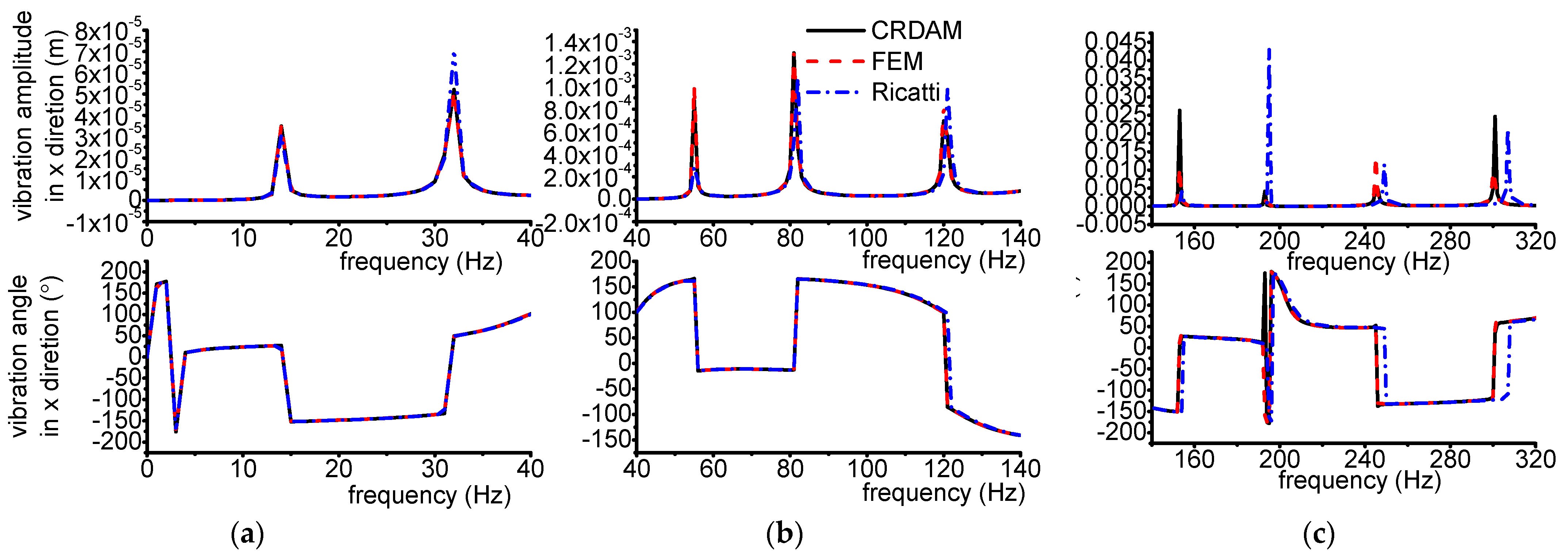
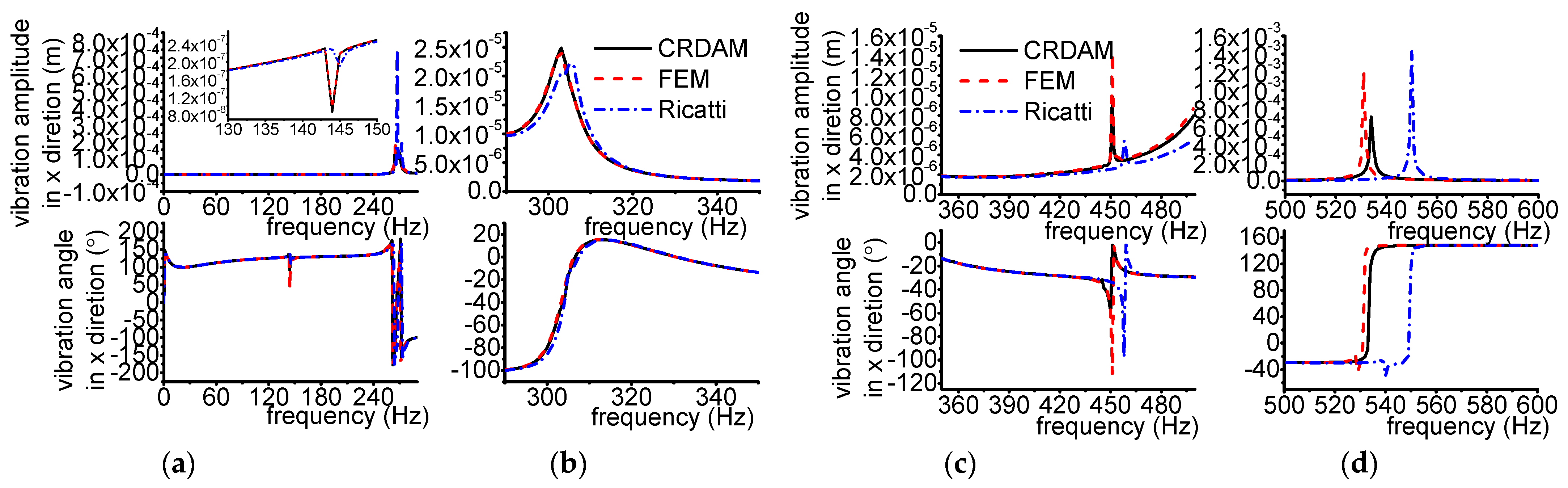
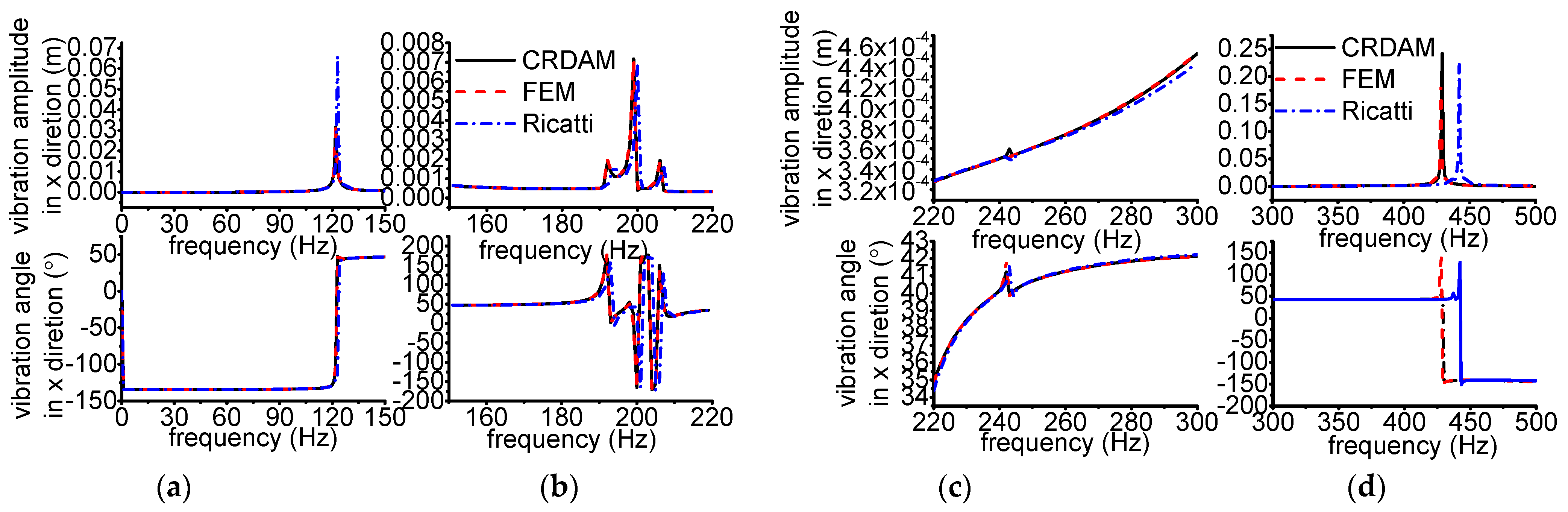
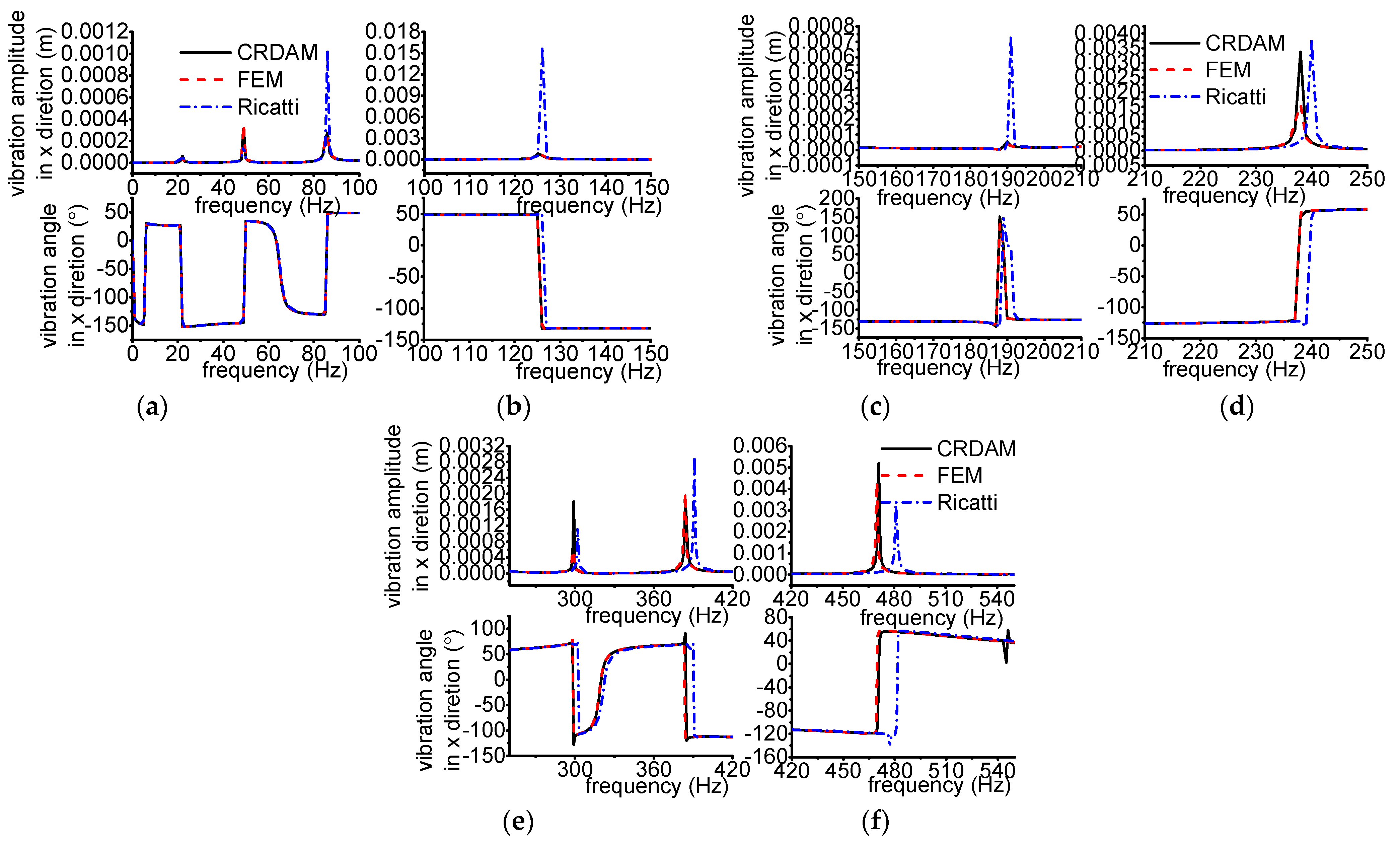
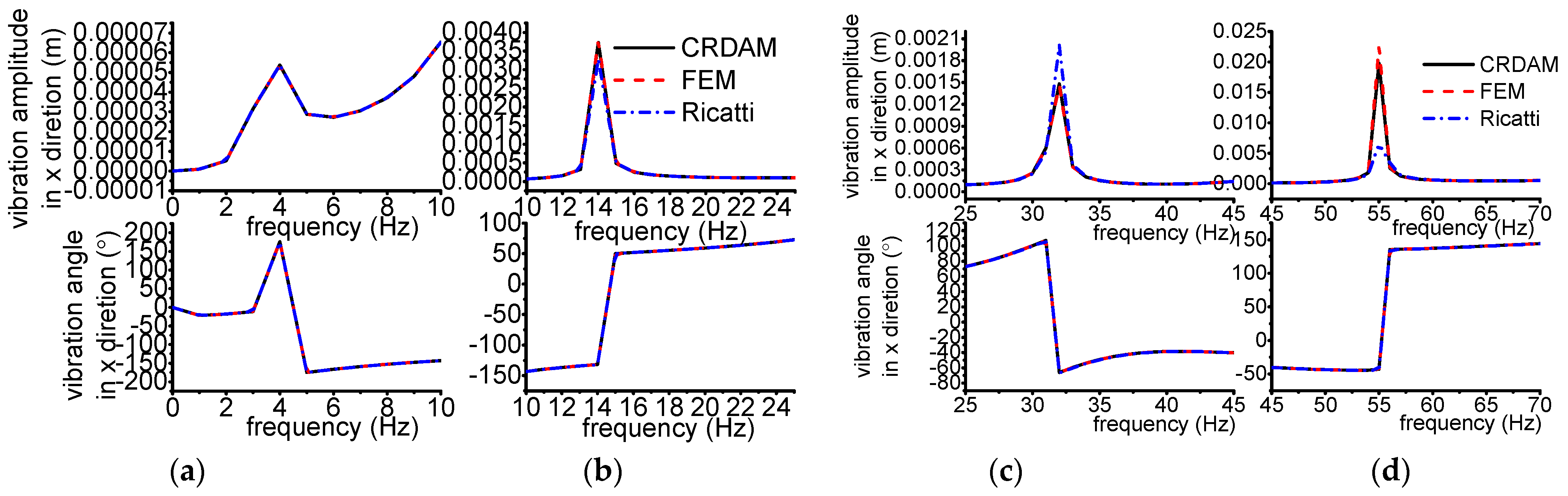
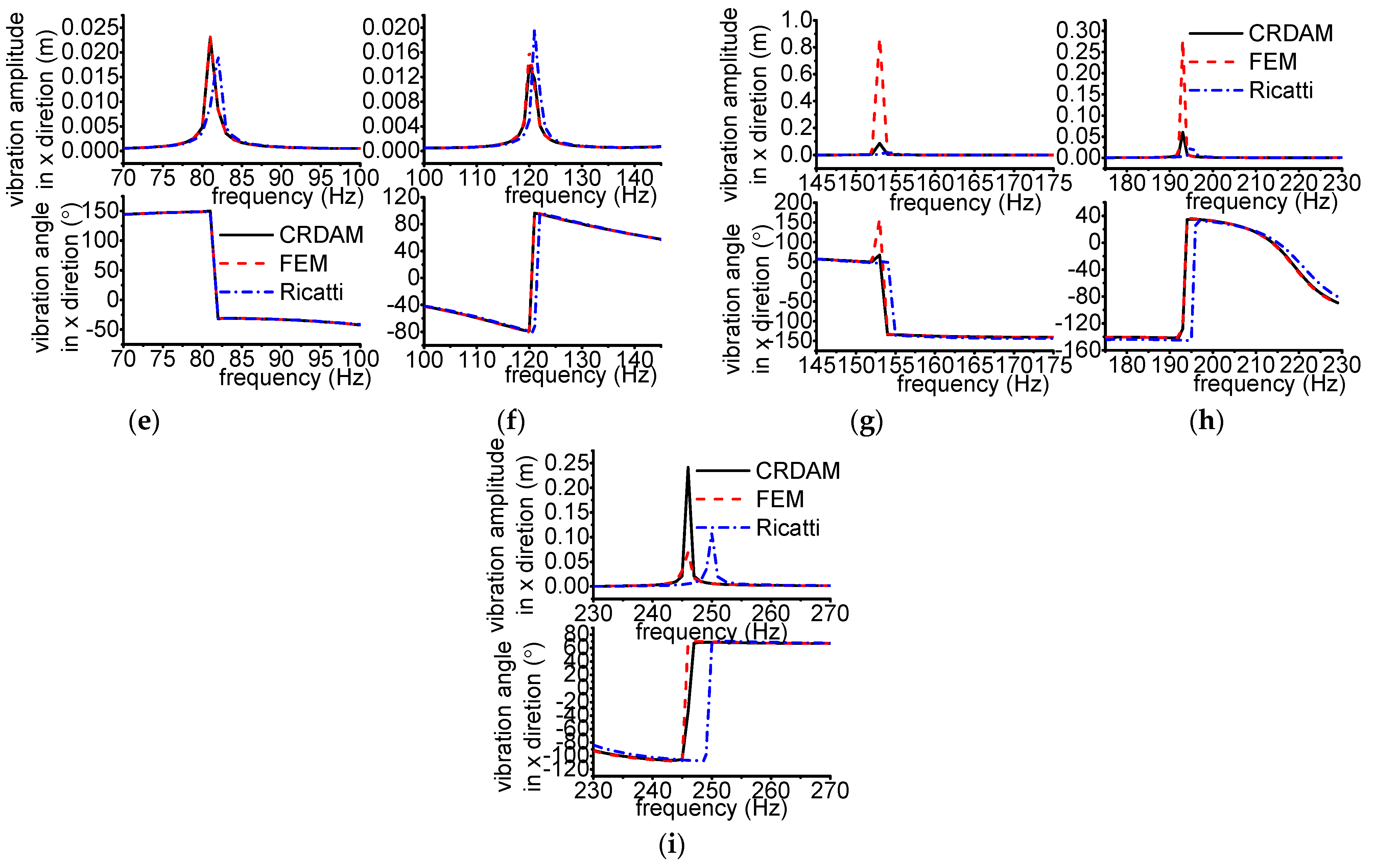
3.3.1. Results
3.3.2. Discussion
- (1)
- Accuracy
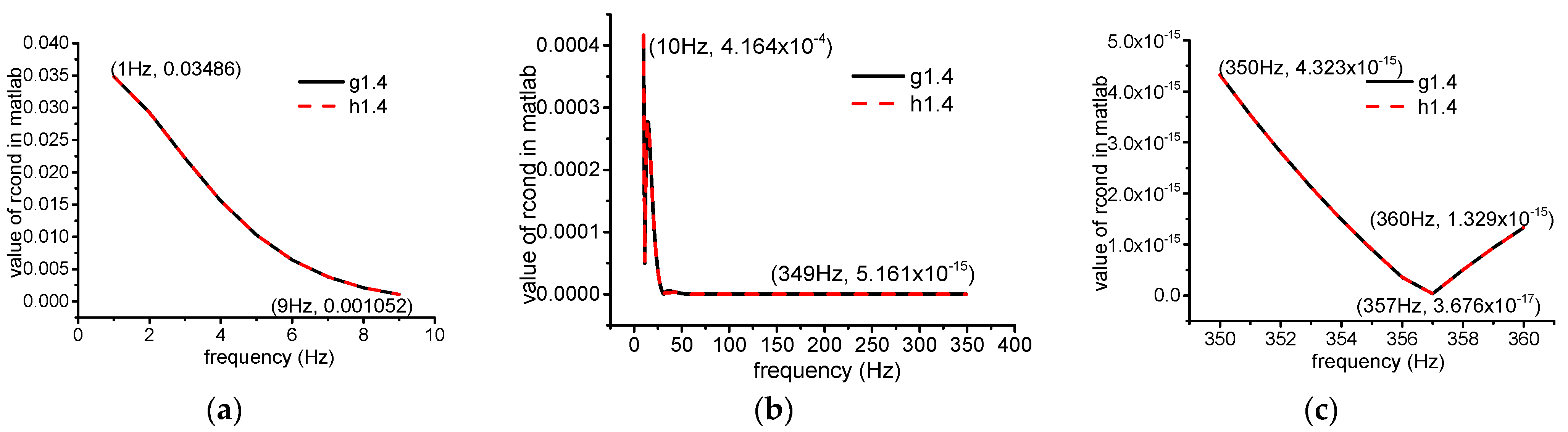
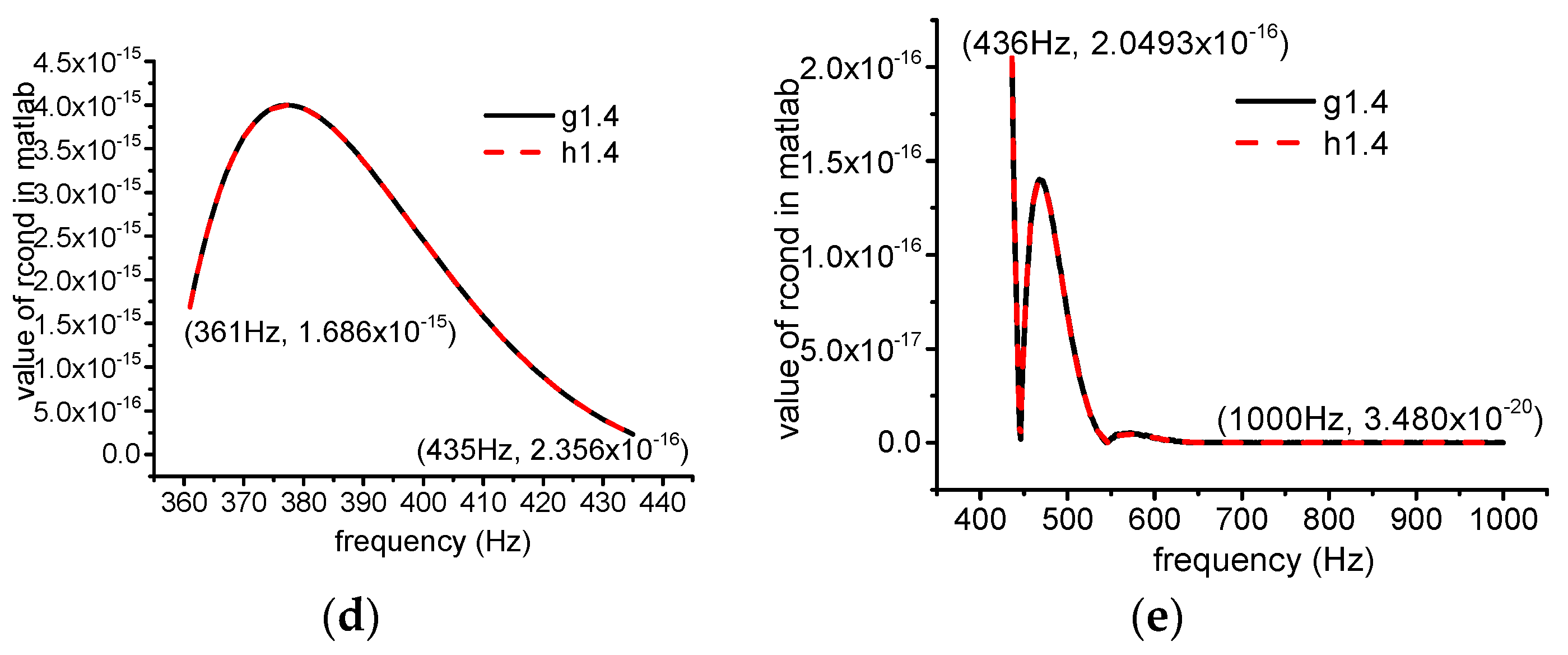
- (2)
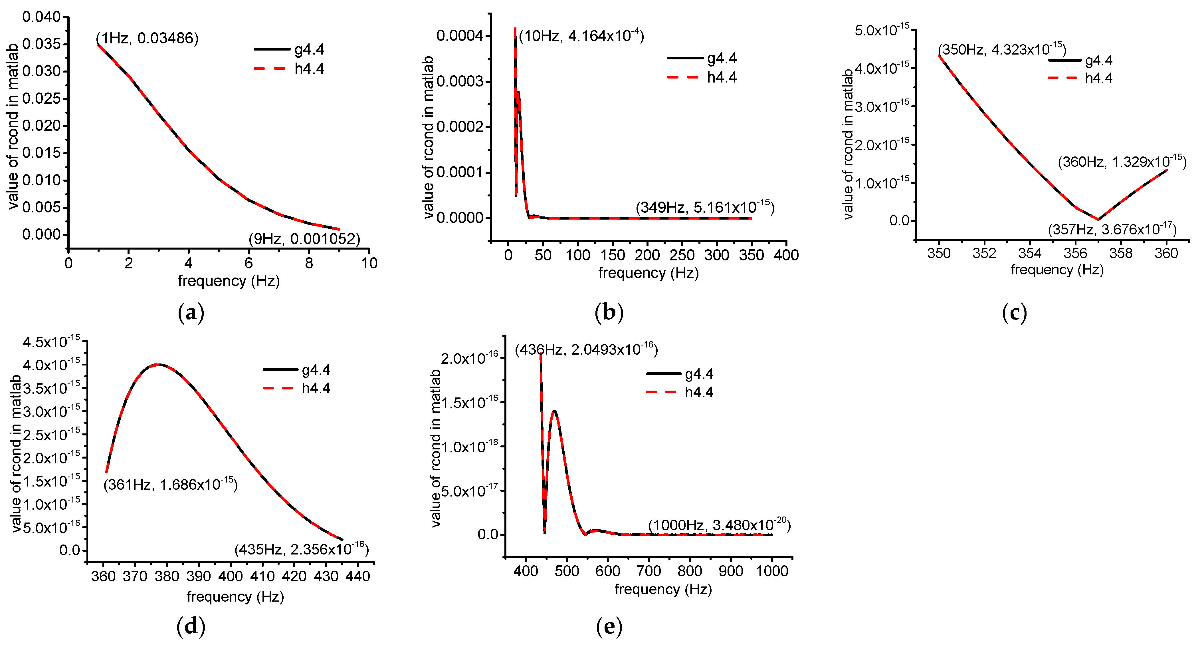
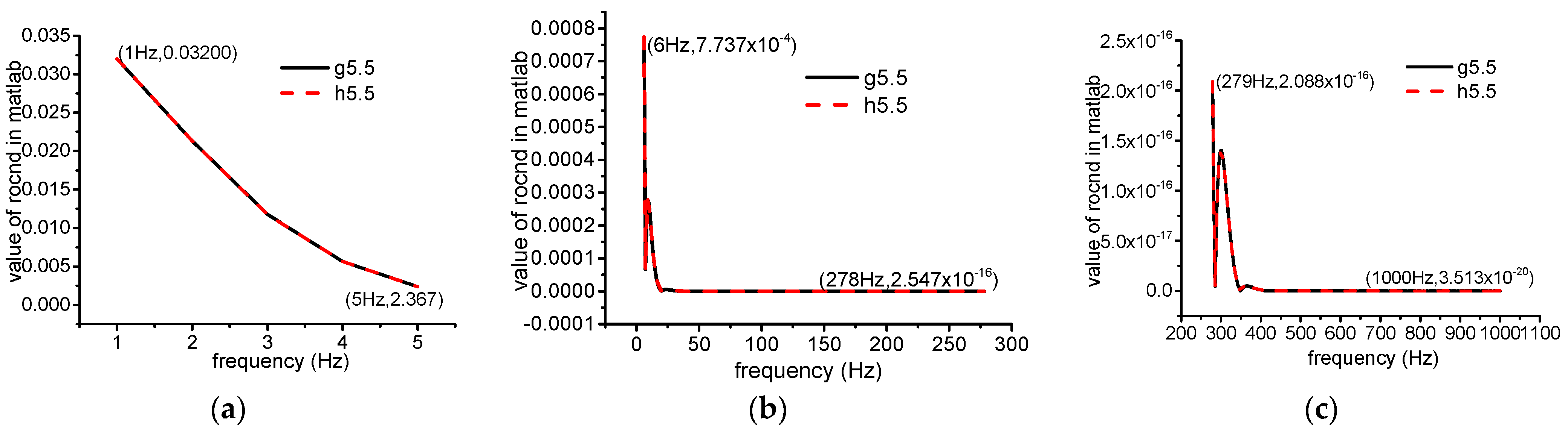
- Numerical stability
3.4. Calculating Speed
4. Conclusions
- (1)
- The functional relationship between the unbalance response and location on the shaft, rotor unbalance (amplitude and angle), each bearing’s stiffness and damping coefficients and rotor’s inherent parameters is obtained based on CRDAM.
- (2)
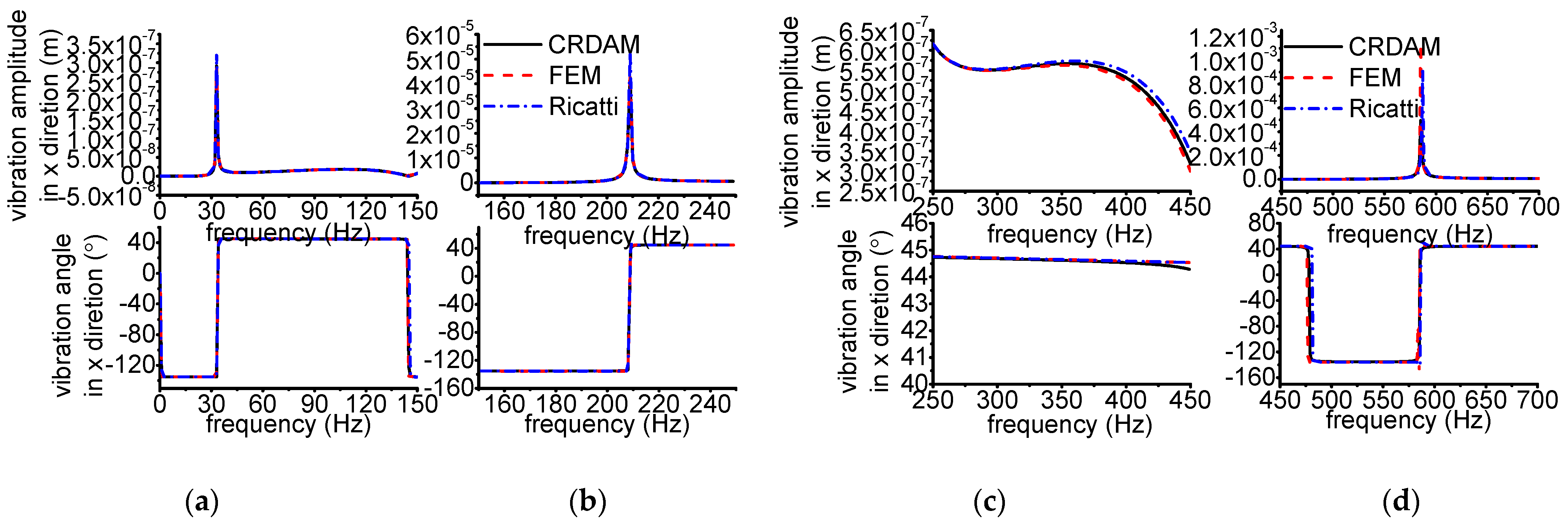
- Numerical simulations indicate that the obtained unbalance response calculated by the three methods are almost equal when the frequency is away from the critical frequency, but they are different when the frequency is near the critical frequency. Moreover, CRDAM is closer to FEM than Ricatti. Although the critical frequencies calculated by them are almost equal to each other, the critical frequency calculated by CRDAM is closer to the critical frequency calculated by FEM than the critical frequency obtained by Ricatti. The unbalance response obtained by CRDAM is also closer to the unbalance response obtained by FEM than the unbalance response by Ricatti, especially when the frequency is smaller than the low order frequency.
- (3)
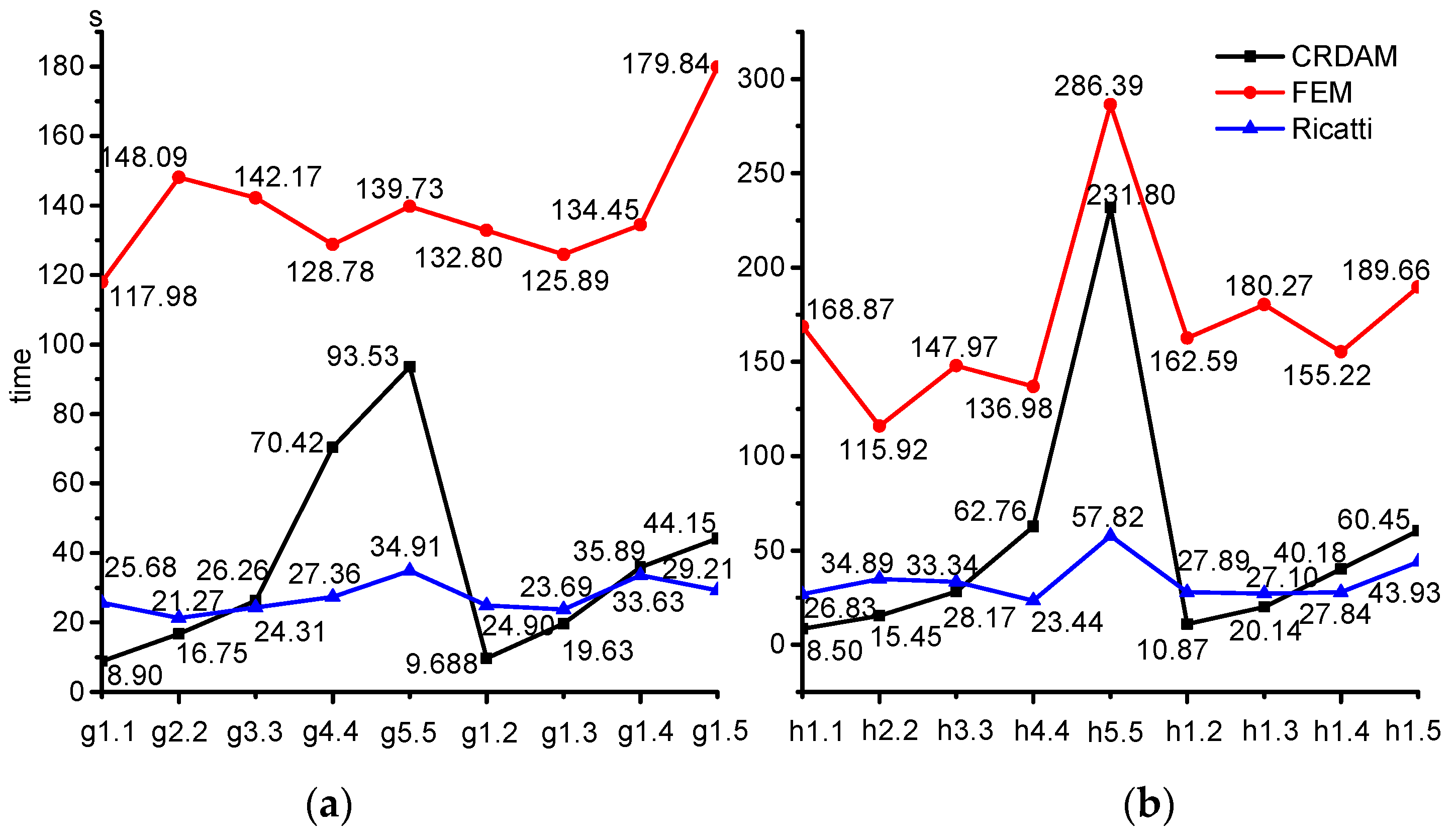
- Numerical simulations indicate that the calculating speed of CRDAM is the second fast among the three methods, but the speed of CRDAM becomes faster than Ricatti when the rotor is complicated. Simulations also show that the numerical stability of FEM and Ricatti is better than CRDAM. However, the numerical instability of CRDAM occurs when the frequency is high, often higher than the fifth order frequency.
Author Contributions
Funding
Institutional Review Board Statement
Informed Consent Statement
Data Availability Statement
Conflicts of Interest
Appendix A
Appendix B

| g1.1 | h1.1 | |||||||||
|---|---|---|---|---|---|---|---|---|---|---|
| Order | CRDAM | FE | Ricatti | C/F(%) | R/F(%) | CRDAM | FEM | Ricatti | C/F(%) | R/F(%) |
| 1th | 33 | 33 | 33 | 0.000 | 0.000 | 33 | 33 | 33 | 0.000 | 0.000 |
| 2th | 209 | 209 | 209 | 0.000 | 0.000 | 212 | 212 | 212 | 0.000 | 0.000 |
| 3th | 355 | 352 | 360 | 0.852 | 2.273 | 598 | 597 | 596 | 0.168 | 0.168 |
| g2.2 | h2.2 | |||||||||
|---|---|---|---|---|---|---|---|---|---|---|
| Order | CRDAM (Hz) | FEM (Hz) | Ricatti (Hz) | C/F (%) | R/F (%) | CRDAM (Hz) | FEM (Hz) | Ricatti (Hz) | C/F (%) | R/F (%) |
| 1th | 16 | 16 | 16 | 0.000 | 0.000 | 16 | 16 | 16 | 0.000 | 0.000 |
| 2th | 104 | 104 | 104 | 0.000 | 0.000 | 104 | 104 | 104 | 0.000 | 0.000 |
| 3th | 294 | 294 | 294 | 0.000 | 0.000 | 295 | 295 | 295 | 0.000 | 0.000 |
| 4th | 568 | 568 | 571 | 0.000 | 0.528 | 570 | 570 | 573 | 0.000 | 0.526 |
| 5th | 774 | 773 | 777 | 0.129 | 0.517 | 799 | 798 | 799 | 0.125 | 0.125 |
| g3.3 | h3.3 | |||||||||
|---|---|---|---|---|---|---|---|---|---|---|
| Order | CRDAM | FE | Ricatti | C/F(%) | R/F(%) | CRDAM | FEM | Ricatti | C/F(%) | R/F(%) |
| 1th | 14 | 14 | 14 | 0.000 | 0.000 | 92 | 92 | 92 | 0.000 | 0.000 |
| 2th | 91 | 91 | 91 | 0.000 | 0.000 | 258 | 258 | 260 | 0.000 | 0.775 |
| 3th | 256 | 256 | 258 | 0.000 | 0.781 | 433 | 433 | 436 | 0.000 | 0.693 |
| 4th | 390 | 390 | 392 | 0.000 | 0.513 | 458 | 457 | 458 | 0.219 | 0.219 |
| 5th | 431 | 431 | 434 | 0.000 | 0.696 | 562 | 562 | 567 | 0.000 | 0.890 |
| 6th | 549 | 549 | 555 | 0.000 | 1.093 | 892 | 892 | 911 | 0.000 | 2.130 |
| 7th | 928 | 916 | 962 | 1.310 | 5.022 | 947 | 934 | 982 | 1.392 | 5.139 |
| g4.4 | h4.4 | |||||||||
|---|---|---|---|---|---|---|---|---|---|---|
| Order | CRDAM | FE | Ricatti | C/F(%) | R/F(%) | CRDAM | FEM | Ricatti | C/F(%) | R/F(%) |
| 1th | 143 | 143 | 144 | 0.000 | 0.699 | 265 | 265 | 267 | 0.000 | 0.755 |
| 2th | 253 | 253 | 255 | 0.000 | 0.791 | 303 | 303 | 305 | 0.000 | 0.660 |
| 3th | 259 | 259 | 260 | 0.000 | 0.386 | 451 | 451 | 458 | 0.000 | 1.552 |
| 4th | 279 | 279 | 280 | 0.000 | 0.358 | 534 | 531 | 550 | 0.565 | 3.578 |
| 5th | 447 | 447 | 454 | 0.000 | 1.566 | / | / | / | / | / |
| 6th | 529 | 526 | 544 | 0.570 | 3.422 | / | / | / | / | / |
| 7th | 739 | 738 | 759 | 0.136 | 2.846 | / | / | / | / | / |
| g5.5 | h5.5 | |||||||||
|---|---|---|---|---|---|---|---|---|---|---|
| Order | CRDAM | FE | Ricatti | C/F(%) | R/F(%) | CRDAM | FEM | Ricatti | C/F(%) | R/F(%) |
| 1th | 171 | 171 | 172 | 0.000 | 0.585 | 122 | 122 | 123 | 0.000 | 0.820 |
| 2th | 341 | 340 | 350 | 0.294 | 2.941 | 192 | 192 | 193 | 0.000 | 0.521 |
| 3th | 484 | 483 | 497 | 0.207 | 2.899 | 199 | 199 | 200 | 0.000 | 0.503 |
| 4th | / | / | / | / | / | 206 | 206 | 207 | 0.000 | 0.485 |
| 5th | / | / | / | / | / | 243 | 241 | 242 | 0.830 | 0.415 |
| 6th | / | / | / | / | / | 429 | 428 | 442 | 0.234 | 3.271 |
| g1.2 | h1.2 | |||||||||
|---|---|---|---|---|---|---|---|---|---|---|
| Order | CRDAM (Hz) | FEM (Hz) | Ricatti (Hz) | C/F (%) | R/F (%) | CRDAM (Hz) | FEM (Hz) | Ricatti (Hz) | C/F (%) | R/F (%) |
| 1th | 22 | 22 | 22 | 0.000 | 0.000 | 22 | 22 | 22 | 0.000 | 0.000 |
| 2th | 87 | 87 | 87 | 0.000 | 0.000 | 87 | 87 | 87 | 0.000 | 0.000 |
| 3th | 198 | 198 | 199 | 0.000 | 0.505 | 198 | 198 | 199 | 0.000 | 0.505 |
| 4th | 329 | 329 | 330 | 0.000 | 0.304 | 329 | 329 | 330 | 0.000 | 0.304 |
| 5th | 517 | 517 | 520 | 0.000 | 0.580 | 518 | 517 | 521 | 0.193 | 0.774 |
| 6th | 749 | 747 | 757 | 0.268 | 1.339 | 753 | 750 | 749 | 0.400 | 0.133 |
| 7th | 952 | 948 | 963 | 0.422 | 1.582 | 965 | 960 | 977 | 0.521 | 1.771 |
| g1.3 | h1.3 | |||||||||
|---|---|---|---|---|---|---|---|---|---|---|
| Order | CRDAM | FE | Ricatti | C/F(%) | R/F(%) | CRDAM | FEM | Ricatti | C/F(%) | R/F(%) |
| 1th | 10 | 10 | 10 | 0.000 | 0.000 | 10 | 10 | 10 | 0.000 | 0.000 |
| 2th | 39 | 39 | 40 | 0.000 | 2.564 | 39 | 39 | 40 | 0.000 | 2.564 |
| 3th | 86 | 86 | 86 | 0.000 | 0.000 | 86 | 86 | 86 | 0.000 | 0.000 |
| 4th | 151 | 151 | 152 | 0.000 | 0.662 | 151 | 151 | 152 | 0.000 | 0.662 |
| 5th | 225 | 225 | 226 | 0.000 | 0.444 | 225 | 225 | 226 | 0.000 | 0.444 |
| 6th | 335 | 334 | 338 | 0.299 | 1.198 | 335 | 335 | 338 | 0.000 | 0.896 |
| 7th | 425 | 424 | 429 | 0.236 | 1.179 | 426 | 425 | 431 | 0.235 | 1.412 |
| 8th | 526 | 525 | 531 | 0.190 | 1.143 | 529 | 529 | 535 | 0.000 | 1.134 |
| 9th | 686 | 683 | 700 | 0.439 | 2.489 | 691 | 688 | 705 | 0.436 | 2.471 |
| 10th | 847 | 843 | 868 | 0.474 | 2.966 | 853 | 848 | 874 | 0.590 | 3.066 |
| g1.4 | h1.4 | |||||||||
|---|---|---|---|---|---|---|---|---|---|---|
| Order | CRDAM | FE | Ricatti | C/F(%) | R/F(%) | CRDAM | FEM | Ricatti | C/F(%) | R/F(%) |
| 1th | 22 | 22 | 22 | 0.000 | 0.000 | 22 | 22 | 22 | 0.000 | 0.000 |
| 2th | 49 | 49 | 49 | 0.000 | 0.000 | 49 | 49 | 49 | 0.000 | 0.000 |
| 3th | 86 | 86 | 86 | 0.000 | 0.000 | 86 | 86 | 86 | 0.000 | 0.000 |
| 4th | 125 | 125 | 126 | 0.000 | 0.800 | 125 | 125 | 126 | 0.000 | 0.800 |
| 5th | 237 | 237 | 239 | 0.000 | 0.844 | 190 | 189 | 191 | 0.529 | 1.058 |
| 6th | 298 | 298 | 301 | 0.000 | 1.007 | 238 | 238 | 240 | 0.000 | 0.840 |
| 7th | 383 | 382 | 389 | 0.262 | 1.832 | 299 | 299 | 302 | 0.000 | 1.003 |
| 8th | 470 | 469 | 480 | 0.213 | 2.345 | 384 | 384 | 391 | 0.000 | 1.823 |
| 9th | / | / | / | / | / | 471 | 470 | 481 | 0.213 | 2.340 |
| g1.5 | h1.5 | |||||||||
|---|---|---|---|---|---|---|---|---|---|---|
| Order | CRDAM | FE | Ricatti | C/F(%) | R/F(%) | CRDAM | FEM | Ricatti | C/F(%) | R/F(%) |
| 1th | 4 | 4 | 4 | 0.000 | 0.000 | 4 | 4 | 4 | 0.000 | 0.000 |
| 2th | 14 | 14 | 14 | 0.000 | 0.000 | 14 | 14 | 14 | 0.000 | 0.000 |
| 3th | 32 | 32 | 32 | 0.000 | 0.000 | 32 | 32 | 32 | 0.000 | 0.000 |
| 4th | 81 | 81 | 82 | 0.000 | 1.235 | 55 | 55 | 55 | 0.000 | 0.000 |
| 5th | 120 | 120 | 121 | 0.000 | 0.833 | 81 | 81 | 82 | 0.000 | 1.235 |
| 6th | 153 | 153 | 154 | 0.000 | 0.654 | 120 | 120 | 121 | 0.000 | 0.833 |
| 7th | 193 | 193 | 194 | 0.000 | 0.518 | 153 | 153 | 154 | 0.000 | 0.654 |
| 8th | 245 | 245 | 249 | 0.000 | 1.633 | 193 | 193 | 195 | 0.000 | 1.036 |
| 9th | 301 | 300 | 307 | 0.333 | 2.333 | 246 | 246 | 250 | 0.000 | 1.626 |
| 10th | / | / | / | / | / | 301 | 301 | 308 | 0.000 | 2.326 |
Appendix C


References
- Horner, G.C.; Pilkey, W.D. The riccati transfer matrix method. J. Mech. Des. Trans. ASME 1978, 100, 297–302. [Google Scholar] [CrossRef]
- Guptak, K.; Guptak, D. Unbalance response of a dual rotor system: Theory and experiment. J. Vib. Acous. Trans. ASME 1993, 115, 427–435. [Google Scholar] [CrossRef]
- Behzad, M.; Mehri, B. Accuracy of the riccati transfer matrix method in rotor dynamic analysis. In Turbo Expo: Power for Land, Sea, and Air; American Society of Mechanical Engineers: New York, NY, USA, 1998; Volume 78668. [Google Scholar]
- Lee, J.W.; Lee, J.Y. An exact transfer matrix expression for bending vibration analysis of a rotating tapered beam. Appl. Math. Model. 2018, 53, 167–188. [Google Scholar] [CrossRef]
- Chen, G.; Zeng, X.; Liu, X.; Rui, X. Transfer matrix method for the free and forced vibration analyses of multi-step timoshenko beams coupled with rigid bodies on springs. Appl. Math. Model. 2020, 87, 152–170. [Google Scholar] [CrossRef]
- Cao, H.; Niu, L.; Xi, S.; Chen, X. Mechanical model development of rolling bearing-rotor systems: A review. Mech. Syst. Signal Process. 2018, 102, 37–58. [Google Scholar] [CrossRef]
- Nelson, H.D.; McVaugh, J.M. The dynamics of rotor-bearing systems using finite elements. J. Eng. Ind. -Trans. ASME 1976, 5, 593–600. [Google Scholar] [CrossRef]
- Fan, H.; Zhang, X. Analysis of Imbalance Response of the Rotor Test Bed. In Proceedings of the 2008 IEEE/ASME International Conference on Advanced Intelligent Mechatronics, Xi’an, China, 2–5 July 2008; Volume 7, pp. 780–785. [Google Scholar]
- Sekhar, A.S.; Prabhu, B.S. Unbalance response of rotors considering the distributed bearing stiffness and damping. In Turbo Expo: Power for Land, Sea, and Air; American Society of Mechanical Engineers: New York, NY, USA, 1994; Volume 78873. [Google Scholar]
- Tan, X.; He, J.; Xi, C.; Deng, X.; Xi, X.; Chen, W.; He, H. Dynamic modeling for rotor-bearing system with electromechanically coupled boundary conditions. Appl. Math. Model. 2021, 91, 280–296. [Google Scholar] [CrossRef]
- Zhou, W.; Qiu, N.; Wang, L.; Gao, B.; Liu, D. Dynamic analysis of a planar multi-stage centrifugal pump rotor system based on a novel coupled model. J. Sound Vib. 2018, 434, 237–260. [Google Scholar] [CrossRef]
- Han, B.; Ding, Q. Forced responses analysis of a rotor system with squeeze film damper during flight maneuvers using finite element method. Mech. Mach. Theory 2018, 122, 233–251. [Google Scholar] [CrossRef]
- Briend, Y.; Dakel, M.; Chatelet, E.; Andrianoely, M.-A.; Dufour, R.; Baudin, S. Effect of multi-frequency parametric excitations on the dynamics of on-board rotor-bearing systems. Mech. Mach. Theory 2020, 145, 103660. [Google Scholar] [CrossRef]
- Fang, T.; Xue, P. Theory of Vibration and Its Application; Northwestern Polytechnical University Press: Xi’an, China, 1998. [Google Scholar]
- Zhang, W. The Theory of Rotor Dynamics; Science Press: Beijing, China, 1990. [Google Scholar]
- Yu, L. Bearing-Rotor System Dynamics; Xi’an Jiao Tong University Press: Xi’an, China, 2001. [Google Scholar]
- Zhong, Y.; He, Y.; Wang, Z.; Li, F. Rotor Dynamics; Tsinghua University Press: Beijing, China, 1987. [Google Scholar]
- Wen, B.; Gu, J.; Xia, S.; Wang, Z. Advanced Rotor Dynamics: Theory, Technology and Application; Machinery Industry Press: Beijing, China, 1999. [Google Scholar]
- Timoshenko, S. Vibration Problems in Engineering; People’s University Press: Beijing, China, 1978. [Google Scholar]
- Vaz, J.C.; de Lima Junior, J.J. Vibration analysis of Euler-Bernoulli beams in multiple steps and different shapes of cross section. J. Vib. Control 2016, 22, 193–204. [Google Scholar] [CrossRef]
- Heydari, H.; Khorram, A. Effects of location and aspect ratio of a flexible disk on natural frequencies and critical speeds of a rotating shaft-disk system. Int. J. Mech. Sci. 2019, 152, 596–612. [Google Scholar] [CrossRef]
- Varanis, M.; Mereles, A.; Silva, A.; Balthazar, J.M.; Tusset, A.M. Rubbing Effect Analysis in a Continuous Rotor Model. In Proceedings of the New Advances in Mechanism and Machine Science; Springer Science and Business Media LLC: Cham, Switzerland, 2018; pp. 387–399. [Google Scholar]
- Zhou, S.; Shi, J. The Analytical Imbalance Response of Jeffcott Rotor During Acceleration. J. Manuf. Sci. Eng. 2000, 123, 299–302. [Google Scholar] [CrossRef]
- Lee, H.P. Divergence of a rotating shaft with an intermediate support and conservative axial loads. Comput. Methods Appl. Mech. Eng. 1993, 110, 317–324. [Google Scholar] [CrossRef]
- Lee, H.P. Dynamic stability of spinning pre-twisted beams. Int. J. Solids Struct. 1994, 31, 2509–2517. [Google Scholar] [CrossRef]
- Lee, H.P. Dynamic stability of spinning beams of unsymmetrical cross-section with distinct end conditions. J. Sound Vib. 1996, 189, 161–171. [Google Scholar] [CrossRef]
- Chun, S.B.; Lee, C.W. Vibration analysis of shaft-bladed disk system by using substructure synthesis and assumed modes method. J. Sound Vib. 1996, 189, 587–608. [Google Scholar] [CrossRef]
- Lee, C.W.; Chun, S.B. Vibration analysis of a rotor with multiple flexible disks using assumed modes method. J. Vib. Acoust. -Trans. ASME 1998, 120, 87–94. [Google Scholar] [CrossRef]
- Hamidi, L.; Piaud, J.B.; Pastorel, H.; Mansour, W.M.; Massoud, M. Modal parameters for cracked rotors: Models and comparisons. J. Sound Vib. 1994, 175, 265–286. [Google Scholar] [CrossRef]
- Wang, A.; Cheng, X.; Meng, G.; Xia, Y.; Wo, L.; Wang, Z. Dynamic analysis and numerical experiments for balancing of the continuous single-disc and single-span rotor-bearing system. Mech. Syst. Signal Process. 2017, 86, 151–176. [Google Scholar] [CrossRef]
- Liao, H. The application of reduced space harmonic balance method for the nonlinear vibration problem in rotor dynamics. Mech. Based Des. Struct. Mach. 2019, 47, 154–174. [Google Scholar] [CrossRef]
- Bouzidi, I.; Hadjoui, A.; Fellah, A. Dynamic analysis of functionally graded rotor-blade system using theclassical version of the finite element method. Mech. Based Des. Struct. Mach. 2020, 49, 1080–1108. [Google Scholar] [CrossRef]
- Wang, A.; Yao, W.; He, K.; Meng, G.; Cheng, X.; Yang, J. Analytical modelling and numerical experiment for simultaneous identifi-cation of unbalance and rolling-bearing coefficients of the continuous single-disc and single-span rotor-bearing system with Rayleigh beam model. Mech. Syst. Signal Process. 2019, 116, 322–346. [Google Scholar] [CrossRef]
- Mereles, A.; Cavalca, K.L. Mathematical modeling of continuous multi-stepped rotor-bearing systems. Appl. Math. Model. 2021, 90, 327–350. [Google Scholar] [CrossRef]
- Mereles, A.; Cavalca, K.L. Modeling of multi-stepped rotor-bearing systems by the continuous segment method. Appl. Math. Model. 2021, 96, 402–430. [Google Scholar] [CrossRef]
- Farghaly, S.H.; El-Sayed, T.A. Exact free vibration of multi-step timoshenko beam system with several attachments. Mech. Syst. Signal Process. 2016, 72, 525–546. [Google Scholar] [CrossRef]
- Afshari, H.; Rahaghi, M.I. Whirling analysis of multi-span multi-stepped rotating shafts. J. Braz. Soc. Mech. Sci. Eng. 2018, 40, 424. [Google Scholar] [CrossRef]
- Afshari, H.; Torabi, K.; Jazi, A.J. Exact closed form solution for whirling analysis of Timoshenko rotors with multiple concentrated masses. Mech. Based Des. Struct. Mach. 2020, 50, 969–992. [Google Scholar] [CrossRef]
- Torabi, K.; Afshari, H.; Najafi, H. Whirling analysis of axial-loaded multi-step Timoshenko rotor carrying concentrated masses. J. Solid Mech. 2017, 9, 138–156. [Google Scholar]
- Rao, D.K.; Swain, A.; Roy, T. Dynamic responses of bidirectional functionally graded rotor shaft. Mech. Based Des. Struct. Mach. 2020, 50, 302–330. [Google Scholar] [CrossRef]
- De Felice, A.; Sorrentino, S. Damping and gyroscopic effects on the stability of parametrically excited continuous rotor systems. Nonlinear Dyn. 2021, 103, 3529–3555. [Google Scholar] [CrossRef]
- Fung, R.F.; Hsu, S.M. Dynamic formulations and energy analysis of rotating flexible-shaft/multi-flexible-disk system with ed-dy-current brake. J. Vib. Acoust. -Trans. ASME 2000, 122, 365–375. [Google Scholar] [CrossRef]
- Rao, S.S. Vibration of Continuous Systems; Wiley: New York, NY, USA, 2007. [Google Scholar]


| Symbols | Description |
|---|---|
| is the dimensionless lateral displacement of the shaft in y direction. | |
| is the dimensionless lateral displacement of the shaft in x direction. | |
| is the dimensionless quantityy of z. | |
| is the dimensionless ; is the position of NO. i bearing; i = 1 − n. | |
| uib is the dimensionless lateral displacement of the shaft in y direction at position zib. | |
| is the dimensionless lateral displacement of the shaft in x direction at position . | |
| is the dimensionless ; is the position of the number j disc; j = 1 − m. | |
| is the dimensionless lateral displacement of the shaft in y direction at position . | |
| is the dimensionless lateral displacement of the shaft in x direction at position . |
| Parameter | Meaning |
|---|---|
| r_shaft | Radius of the shaft |
| p_shaft | Density of the shaft |
| E_shaft | Elastic modulus of the shaft |
| L_shaft | Length of the shaft |
| r_disc | Radius of the disc |
| p_disc | Density of the disc |
| E_disc | Elastic modulus of the disc |
| L_disc | Width of the disc |
| Parameter | Value | Parameter | Value |
|---|---|---|---|
| r_shaft | 10 × 10−3 m | L_shaft of h4.4, h1.4, g4.4, g1.4 | 1800 × 4 × 10−3 m |
| p_shaft | 7800 kg·m−3 | L_shaft of h3.3, h1.3, g3.3, g1.3 | 1800 × 3 × 10−3 m |
| E_shaft | 2.1 × 10¹¹ Pa | L_shaft of h2.2, h1.2, g2.2, g1.2 | 1800 × 2 × 10−3 m |
| L_shaft of h5.5, h1.5, g5.5, g1.5 | 1800 × 5 × 10−3 m | L_shaft of h1.1, g1.1 | 1800 × 1 × 10−3 m |
| Parameter | Value | Parameter | Value | Parameter | Value |
|---|---|---|---|---|---|
| 0.05 kg | 0.15 kg | 0.01 kg | |||
| 30 × 10−3 m | 10 × 10−3 m | 20 × 10−3 m | |||
| 45° | 90° | 20° | |||
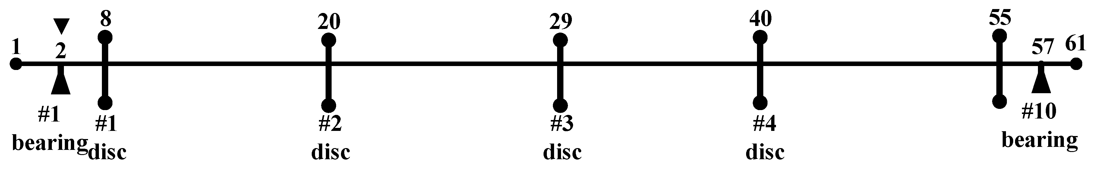
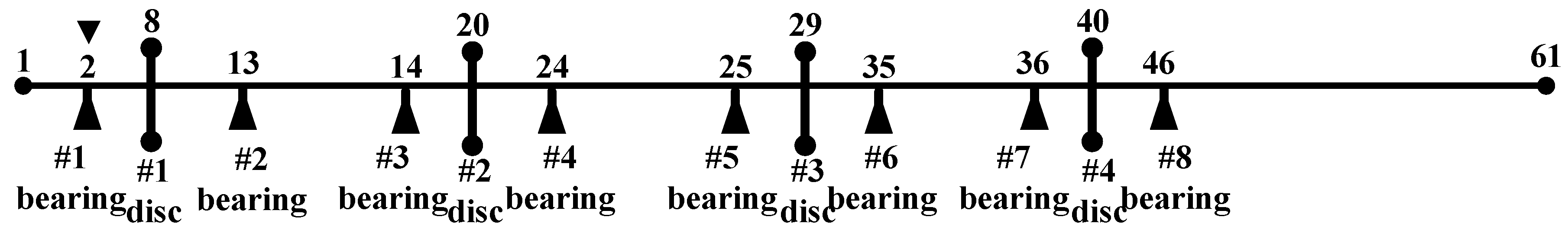
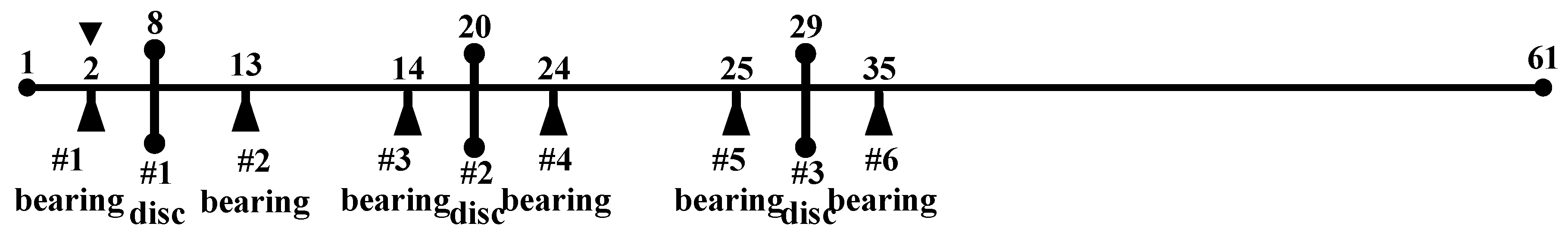
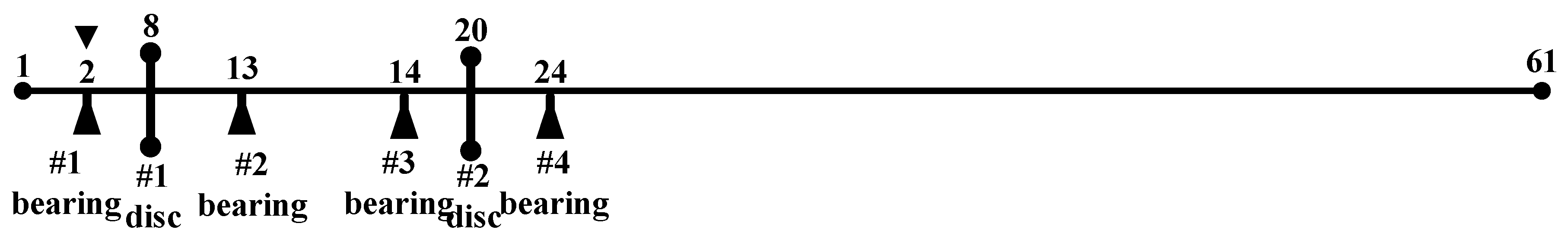
| Z1d | Point 8 | Z2d | Point 20 | Z3d | Point 29 |
| 0.10 kg | 0.05 kg | r_disc of #1~#5 disc | 50 × 10−3 m | ||
| 15 × 10−3 m | 40 × 10−3 m | p_disc of of #1~#5 disc | 7800 kg·m−3 | ||
| 190° | 290° | E_disc of of #1~#5 disc | 2.1 × 10¹¹ Pa | ||
| Z4d | Point 40 | Z5d | Point 55 | L_disc of of #1~#5 disc | 10 × 10−3 m |
| Parameter | Value | Parameter | Value |
|---|---|---|---|
| N/m | |||
| N·s/m | N·s/m | ||
| N/m | |||
| N·s/m | N·s/m | ||
| N/m | |||
| N·s/m | N·s/m | ||
| N/m | |||
| N·s/m | N·s/m | ||
| N/m | |||
| N·s/m | |||
| Z1b | Point 2 | Z2b | Point 13 |
| Z3b | Point 14 | Z4b | Point 24 |
| Z5b | Point 25 | Z6b | Point 35 |
| Z7b | Point 36 | Z8b | Point 46 |
| Z9b | Point 47 | Z10b | Point 57 |
| Z1b | Z2b | Z3b | Z4b | Z5b | Z6b | Z7b | Z8b |
|---|---|---|---|---|---|---|---|
| Point 2 | Point 13 | Point 14 | Point 24 | Point 25 | Point 35 | Point 36 | Point 46 |
| Z9b | Z10b | , i = 1 to 10 | |||||
| Point 47 | Point 57 | N/m | N·s/m | ||||
Publisher’s Note: MDPI stays neutral with regard to jurisdictional claims in published maps and institutional affiliations. |
© 2022 by the authors. Licensee MDPI, Basel, Switzerland. This article is an open access article distributed under the terms and conditions of the Creative Commons Attribution (CC BY) license (https://creativecommons.org/licenses/by/4.0/).
Share and Cite
Wang, A.; Bi, Y.; Xia, Y.; Cheng, X.; Yang, J.; Meng, G. Continuous Rotor Dynamics of Multi-Disc and Multi-Span Rotor: A Theoretical and Numerical Investigation on the Continuous Model and Analytical Solution for Unbalance Responses. Appl. Sci. 2022, 12, 4351. https://doi.org/10.3390/app12094351
Wang A, Bi Y, Xia Y, Cheng X, Yang J, Meng G. Continuous Rotor Dynamics of Multi-Disc and Multi-Span Rotor: A Theoretical and Numerical Investigation on the Continuous Model and Analytical Solution for Unbalance Responses. Applied Sciences. 2022; 12(9):4351. https://doi.org/10.3390/app12094351
Chicago/Turabian StyleWang, Aiming, Yujie Bi, Yun Xia, Xiaohan Cheng, Jie Yang, and Guoying Meng. 2022. "Continuous Rotor Dynamics of Multi-Disc and Multi-Span Rotor: A Theoretical and Numerical Investigation on the Continuous Model and Analytical Solution for Unbalance Responses" Applied Sciences 12, no. 9: 4351. https://doi.org/10.3390/app12094351