Article

Real-Time Power Management Including an Optimization Problem for PV-Powered Electric Vehicle Charging Stations

by
Saleh Cheikh-Mohamad
,
Manuela Sechilariu
* and
Fabrice Locment
AVENUES, Université de Technologie de Compiègne, Centre Pierre Guillaumat-CS 60 319, 60203 Compiègne, France
*
Author to whom correspondence should be addressed.
Appl. Sci. 2022, 12(9), 4323; https://doi.org/10.3390/app12094323
Submission received: 31 March 2022 / Revised: 20 April 2022 / Accepted: 22 April 2022 / Published: 25 April 2022

Abstract

:

Featured Application

This article presents real-time power management including an optimization problem, formulated as mixed-integer linear programming, for a microgrid-based intelligent infrastructure for recharging electric vehicles (EVs). The DC microgrid includes photovoltaic sources, stationary storage, a power grid connection, and EV batteries as load. The objective of the optimization problem is to minimize the total energy cost. Simulation and real-time experimental results under different meteorological conditions prove the feasibility of the proposed control and its superiority over the storage priority strategy.

Abstract

Electric vehicles (EVs) are expanding quickly and widely, and, therefore, EVs can participate in reducing direct greenhouse gas emissions. The intelligent infrastructure for recharging EVs, which is microgrid-based, includes photovoltaic (PV) sources, stationary storage, and a grid connection as power sources. In this article, the energy cost optimization problem is studied, taking into account the intermittent arrival and departure of EVs. A mixed-integer linear programming is formulated as an optimization problem in a real-time operation to minimize the total energy cost, taking into consideration the physical limitations of the system. The interaction with the human-machine interface provides EV data in real-time operation, and the prediction only communicates the PV prediction profile provided by the national meteorological institute in France. The optimization is executed at each EV arrival, with the actualized data in the DC microgrid. Simulation and real-time experimental results of different meteorological conditions show that the EV user demands are satisfied, proving the feasibility of the proposed optimization problem for real-time power management.

1. Introduction

CO2 emissions are the major issue of global warming. The transport sector shares 25% of the global energy consumption in the world and therefore contributes to these emissions [1,2]. Renewable energies can decrease greenhouse gases and, therefore, CO2 emissions due to pollution from the electrical power plants running on fossil fuels. In this context, the energy transition promotes the growth of renewable energy sources; however, this transition can introduce new constraints for grid operators in terms of reliability and quality [
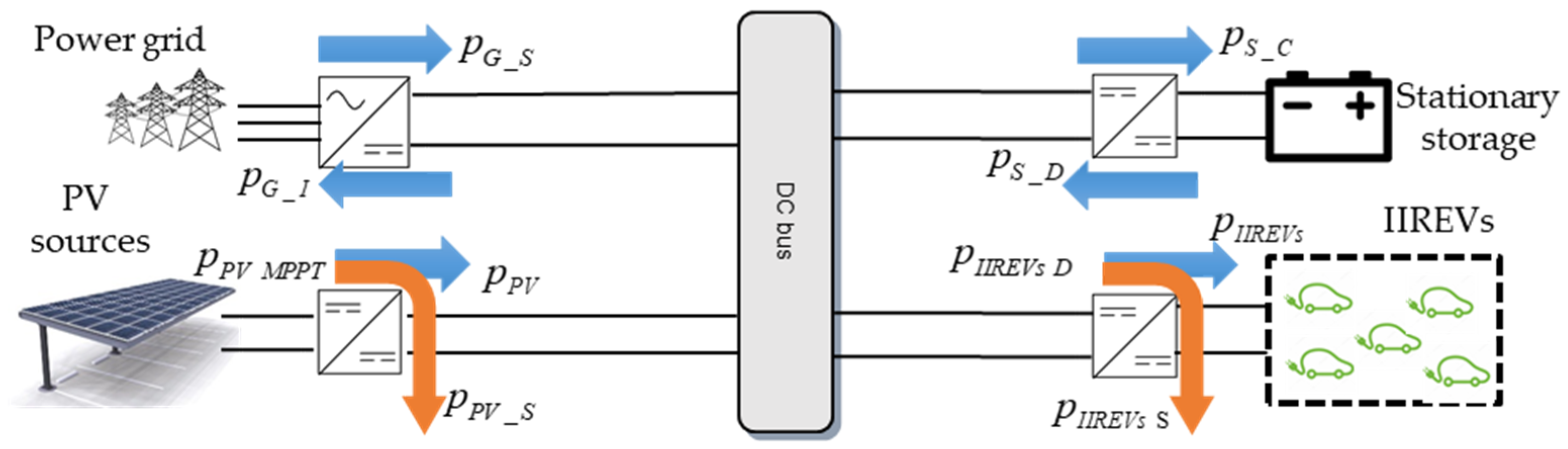
3]. Therefore, microgrids are able to balance local production and consumption of energy and bring benefits to end-user by reducing electricity costs, e.g., reduced transmission cost and distribution cost by lowest energy loss in transmission. Microgrids are based on renewable energy sources such as photovoltaics (PV) and wind, storage devices, and loads and could have a connection to the grid [4]. Electric vehicles (EVs) have been a center of attention worldwide due to their merits: zero tailpipe emissions, noise-free operation, high efficiency of energy use and simple structure [5,6]. The EV market is constantly growing [1,7,8]. However, the increase in EV charging, seen as loads connected to the grid, will have a significant impact on the grid and will impose additional difficulties for grid operators [9,10]. Therefore, managing EV charging will be a critical requirement.

1.1. Literature Review

Recent studies have aimed to design microgrids for EV charging. The authors of [11] have proposed mixed-integer linear programming (MILP) for an EV charging station integrated into a DC microgrid to determine the optimal operation planning. They have focused on optimizing the daily operational costs based on forecasting PV production and EV operation. A hybrid optimization problem for energy storage management has been proposed in [12] to minimize the EV charging cost in a PV-integrated EV charging station using time-of-use wholesale electricity pricing. The authors in [13] have presented meta-heuristic methods, such as binary particle swarm optimization and binary grey wolf optimization. They have studied an optimal charging coordination strategy for a random arrival of plug-in EVs. A MILP optimization has been proposed in [14] to minimize the microgrid operation cost by having an aggregated EV charging station for an islanded microgrid and in [15] to minimize the energy generation cost and load shedding considering various constraints in a microgrid that integrates battery EV charging stations. A heuristic operation problem has been proposed in [2] for a commercial building microgrid that integrates EVs and a PV system to study a strategy to acquire data in real-time rather than forecasting EV charging demand or PV production. A genetic algorithm optimization has been studied in [16] for the multi-criteria optimization problem to minimize the charging costs of the EV, maximize the use of PV and the storage device and minimize the degradation of the storage device. A MILP optimization has been proposed in [17] to solve the day-ahead optimization problem and to find the optimal scheduling and operation of a prosumer who owns renewable energy sources and a plugged-in EV. They have used a feed-forward artificial neural network for the weather prediction module in the energy management system. Linear programming and quadratic programming optimization problems have been addressed in [18] to minimize the total operating costs for building a microgrid that integrates a heterogeneous fleet of EVs. A multi-objective scheduling optimization problem based on genetic algorithms has been presented in [19] for microgrids including EVs to reduce grid loss and charging costs considering various constraints of the microgrid sources and EV charging characteristics. The authors in [20] have presented an optimal model for an energy management strategy in a real microgrid, which integrates a PV system with storage devices, smart buildings and a plug-in EV. They have minimized the total costs of energy consumption by reducing the power supplied from the grid. A robust optimization has been described in [21] and compared with stochastic optimization to minimize the economic and environmental costs of a microgrid, which integrates PV and EVs. They have proposed a mathematical model to study the uncertainty of EV charging behavior and PV power. A model predictive control has been depicted in [22] using a smart charging strategy that takes into account the future EV charging demand. Their goal is to reduce the peak energy demand for an EV parking lot with PV sources. A multi-objective evolutionary particle swarm optimization problem has been presented in [23] to minimize the costs and the overloading for high demands of grid energy for EV scheduling based on a day-ahead scenario.
A novel convex quadratic objective function has been proposed in [24] to minimize the power loss of a microgrid in a two-stage optimization method with different penetration levels of plug-in hybrid EVs, studying the behavior of the plug-in hybrid EVs. The authors of [25] have proposed a stochastic planning model as a convex programming problem to optimize the component sizes by minimizing the total cost of the EV charging station considering the uncertainties of PV production, EV charging demand, and different constraints. An improved optimal sizing methodology of a typical residential microgrid integrating renewable energy sources and EVs has been proposed in [26] to lower greenhouse gases emissions and minimize the cost. An annealing mutation particle swarm optimization problem has been studied in [27] for microgrid optimal dispatching to minimize the environmental protection cost and the operation and maintenance cost of a microgrid in a multi-objective economic dispatch model. A multi-agent particle swarm optimization problem has been addressed in [28] for a grid-connected PV, energy storage system and EV charging station to size the PV and the energy storage system and to set the charging/discharging pattern of the energy storage system. The EV charging station integrates PV, an energy storage system and a grid connection. A machine learning-based approach has been proposed in [29] for energy management in a microgrid, taking into account a reconfigurable structure based on remote switching of ties and sectionalizing. They have also proposed a new modified optimization problem based on dragonfly due to the complexity of the problem. An optimal configuration of PV-powered EV charging stations in [30] has been studied economically and technically under different solar irradiation profiles in Vietnam using the HOMER Grid program. An optimization model based on a genetic algorithm has been proposed in [31] to optimize the use and scheduling of energy sources for an intelligent hybrid energy system, including EVs and a micro-combined heat and power system. In [32], a bi-level robust optimization has been proposed to optimize the design of an EV charging station with distributed energy resources. The authors of [33] have proposed an optimization model for a battery-swapping station to minimize the charging cost of EVs by optimizing the charging schedule for swapped EV batteries. An optimal charging profile has been proposed in [34] for EVs to minimize battery degradation and extend their lifetime.
A robust optimal power management system has been presented in [35] for a standalone hybrid AC/DC microgrid. The optimization problem, formulated as a MILP problem, is responsible for supervising the power flow in the hybrid microgrid, with the objective to satisfy the load demand while maximizing the usage of renewable sources (PV and wind), minimizing the usage of diesel generation, extending battery life, and limiting the utilization of the converter between the AC and DC microgrids. An energy management system for a grid-connected microgrid has been addressed in [36] based on a MILP problem to minimize the total energy cost over 24 h, taking into account load demand, grid tariffs, and renewable energy sources production. A long short-term memory network has been proposed in their paper to deal with the power prediction of the renewable energy sources and the load demand, where each hour, it predicts the profiles for the next 24 h. Then, real-time implementation is enabled by the receding horizon strategy, which is used to minimize the prediction error and gives commands for the first hour; then, each hour, the data are actualized. The proposed strategy in [36] proved its cost reduction in comparison with an offline optimization after conducting simulation tests. In [37], a novel modular modeling method has been described for an energy management system for urban multi-energy sources, including cooling, heating and renewable sources, that allow complex system topologies to be modeled. They have conducted various case studies with different climate conditions and electrical loads. They have also compared the results with a rule-based algorithm to compare the annual cost reductions. In [38], the authors have investigated the technical, economic, and environmental aspects of renewable energy sources in a microgrid. An equilibrium optimization problem was developed to minimize the operational cost of the microgrid, which includes PV, wind turbines, and a biomass generator. The simulation results proved the benefits of using the proposed algorithm in reducing operational costs and emissions. An equilibrium optimization problem has been addressed in [39] for optimum PV-storage system integration in a radial distribution network. Multi-objective functions have been addressed to minimize the cost of investment in PV and storage system installations, their cost of operation, the cost of energy not supplied, the power losses in the distribution lines, and the CO2 emissions by the PV and the grid. The proposed method is compared with various techniques to prove its effectiveness. In [40], the authors have proposed an equilibrium algorithm to optimally find the lithium-ion battery parameters, formulated as a nonlinear optimization problem. The proposed method was compared with various recent techniques to prove its accuracy; also, it has proved its closeness to the experimental measurement. An artificial hummingbird optimization technique has been presented in [41] to find the unknown parameters of lithium-ion batteries used in EVs. The proposed method is compared with various recent techniques to prove its value and effectiveness. An experimental test was conducted, and the proposed technique had the highest degree of precision among the other techniques.

1.2. Research Gaps

In the previously cited references, the optimization was performed knowing the EV charging prediction profile for the entire day as day-ahead planning. Knowing an EV charging prediction profile is based on contextual assumptions, e.g., schedule according to the occupancy of a car park or the average EV autonomy, which are not yet validated in the real world. In this work, the objective is to perform a real-time control under optimization for the minimum energy cost and the maximum PV energy for each EV for an intelligent infrastructure for recharging electric vehicles (IIREVs) considering the intermittent and random arrival of the EVs, featuring the EV users’ interaction. For the current work, the optimization is performed more realistically at every random arrival of an EV. Therefore, when a new EV comes to the station, the state of charge ( s o c S ) of the stationary storage and the current state of charge of EVs ( s o c E V v ) in charge are actualized for suitable optimization.

1.3. Contributions

The main contributions of this work are:
  • Proposing EV power profiles, which are based on the EV users’ interaction with the human-machine interface (HMI);
  • Proposing a new method of real-time power management, including energy cost and PV energy optimization for the IIREVs considering the intermittent and random arrival of EVs, where the optimization is performed at each EV arrival;
  • The analysis of the energy distribution by source category for EV charging and the entire station energy system;
  • The validation of the proposed control in simulation and real-time experimental tests in different meteorological conditions and random EV power profiles.
This article is organized as follows. Section 2 presents the control system for the IIREVs, then the MILP optimization problem is detailed with the constraints and the objective function. Section 3 shows the simulation results and analyses for the different case studies. Section 4 presents the results obtained by real-time experimental tests. Finally, the conclusions and further works are presented in Section 5.

2. Supervisory and Control System Based on Real-Time Power Management

Figure 1 shows the DC microgrid, denoted as IIREVs, and includes PV sources, stationary storage, power grid connection, and EVs as DC loads. Two operation modes exist for the PV sources: maximum power point tracking (MPPT), where maximum power is drawn using a perturb and observe algorithm, and PV power limitation, where PV power is limited in case of a surplus of PV power production [42] because the excess power can no longer be fully injected into the storage and/or into the grid. The stationary storage is a backup source acting as an energy reservoir when there is insufficient PV power to charge the EVs. When there is insufficient PV power to charge the EVs, the grid ensures the security of the system by injecting power to the EVs if the stationary storage has reached its lower limits (empty or minimum discharge power). On the other hand, the DC microgrid can sell power to the grid by injecting it when there is a surplus of PV power production and the stationary storage has reached its higher limits (full or maximum charging power) [43]. Regarding the EVs charging, they can operate in two modes: fully charging as requested by their users and EV shedding when it is not possible to fully supply the EVs.
The power flow for IIREVs is shown in Figure 1, where p P V   M P P T is the PV MPPT power, p P V is the PV power, p P V _ S is the PV shed power, p G _ I is the grid injection power, p G _ S is the grid supply power, p S _ C is the stationary storage charging power, p S _ D is the stationary storage discharging power, p I I R E V s   D is the IIREVs’ total demand power, p I I R E V s is the IIREVs’ total power, and p I I R E V s   S is the IIREVs’ shed power. The components of the IIREVs are coupled through their dedicated converters to the common DC bus. PV sources are connected to the DC bus through the DC/DC converter to draw the MPPT power. The stationary storage is connected through a reversible DC/DC converter. The EVs’ batteries, as DC loads, are connected through the DC/DC converter. The grid is connected through a three-phase bidirectional AC/DC converter. It is necessary to ensure power at all times and mitigate the power difference between the power production and the EVs’ demand.
The supervisory control system for the IIREVs is shown in Figure 2. The supervisory and control system consists of four layers: prediction, energy cost optimization, operation, and HMI. The design and implementation of the IIREVs’ control are based on the interaction between the EV users and DC microgrid. Energy cost optimization and operation layers form the control block that should keep the power balanced.
The prediction layer is based on weather forecasts. The energy cost optimization is based on the production prediction and consumption profile. They are calculated based on data from the prediction layer and the interaction with the HMI. From the prediction layer, messages from the smart grid about energy system limits, grid power limits, and dynamic energy pricing are communicated. From the interaction with the HMI, the EV users choose their charging mode ( M v ), desired state of charge of their EV at departure ( S O C E V _ d e s v ) in real-time, and get the state of charge of their EV at arrival ( S O C E V _ a r r v ). MILP optimization is used for the technical-economic dispatching of the microgrid sources and load. This supervisory control has the advantage of interacting with the EV users to perform the optimization; however, if the choices of the EV users are not feasible, they have to change them in order to perform the optimization [44].
The main challenge lies in dealing with the discrete events coming from the HMI. The optimization results communicate the predictive control settings to the operation layer and update the smart grid about the power references of the stationary storage and the power grid. The operation layer holds the algorithm that keeps the power balanced with respect to the constraints of the system and its physical limits [4]; it sets the PV power limitation and performs EV shedding if needed.

2.1. Prediction Layer

Météo France provides hourly predictions allowing the calculation of PV power prediction, which is based on solar irradiation (g) and ambient temperature ( T a m b ) forecast data [45]. The PV power prediction p P V   M P P T   p r e d is calculated in MPPT mode for each time instant t i [46] as given in following equations:
p P V   M P P T   p r e d ( t i ) = P P V _ S T C g ( t i ) 1000 [ 1 + γ ( T P V ( t i ) 25 ) ] N P V   w i t h t i = { t 0 , t 0 + Δ t , t 0 + 2 Δ t , , t F } ,
T P V ( t i ) = T a m b ( t i ) + g ( t i ) N O C T T a i r t e s t G t e s t ,
where P P V _ S T C is the PV power under standard test conditions (STC), γ is the power temperature coefficient (−0.29%/°C), T P V is the PV cell temperature, N P V is the number of PV panels, t 0 , Δ t , and t F are the initial time instant, time interval between two samples, and time instant at the end of time operation, respectively, N O C T is the nominal operating cell temperature (41 °C), T a i r t e s t is the fixed air temperature (20 °C), and G t e s t is the fixed solar irradiation (800 W/m2).

2.2. Human-Machine Interface

As for the EVs, it is possible to charge them in three modes: slow, average, and fast. All EVs can handle up to fast mode, and they are considered to have the same energy capacity. The HMI allows the EV users to set their S O C E V _ a r r v , M v , and S O C E V _ d e s v , and, therefore, the estimated charging time, t e s t _ c h v , which is the required time to reach S O C E V _ d e s v , is calculated as given in (3):
t e s t _ c h v = ( S O C E V _ d e s v S O C E V _ a r r v ) E P E V _ m a x v ,
where E is the EV’s battery capacity, and P E V _ m a x v is the maximum charging power based on the charging mode set by the EV user. The HMI for the IIREVs is shown in Figure 3 and is well explained in detail in [47].

2.3. Energy Cost Optimization

The energy cost optimization layer interacts with the prediction layer and the HMI to run the optimization. The objective of the optimization is to find the lowest energy cost and the maximum PV power for each EV. The sharing power between the stationary storage and the grid is represented by the power distribution coefficient k D that is calculated from this layer using the power references obtained in the optimization. The benefits of optimization lie in many aspects: reducing the grid peak power consumption, minimizing the energy cost, deciding which of the stationary storage or grid may have the better contribution, and avoiding EV and PV shedding. The communication with the smart grid informs the system about grid power limits for injection and supply, which are set by a contract with the grid operators, and the energy pricing in real-time. Additionally, stationary storage physical limits should be known. The objective is to minimize the total energy cost with respect to different constraints [45].
The constraints and the objective function are represented in the following subsections.

2.3.1. PV Sources

The two operation modes for the PV are MPPT and limited power. The PV power that must be shed is noted as p P V _ S . Therefore, p P V is calculated [45] as given by (4):
p P V ( t i ) = p P V   M P P T ( t i ) p P V _ S ( t i ) ,
where p P V _ S = 0 is in MPPT mode; it should not be negative in power limitation mode. Thus, constraints are added as follows:
p P V ( t i ) 0 ,
0 p P V _ S ( t i ) p P V   M P P T ( t i ) .

2.3.2. Stationary Storage

The stationary storage, represented by lithium-ion batteries, must be protected from overcharging and over-discharging; thus the maximum storage power P S _ m a x and the maximum and minimum state of charge of the storage S O C S _ m a x and S O C S _ m i n must be respected to extend the storage lifetime [45,48] as given by (7) and (8). The simplified state of the charge of the storage s o c S evolution [43] is given by (9) for simplicity, where self-discharge and temperature are not considered:
P S _ m a x p S ( t i ) P S _ m a x ,
S O C S _ m i n s o c S ( t i ) S O C S _ m a x ,
s o c S ( t i ) = S O C S 0 + 1 3600 E B a t t 0 t   p S ( t i ) d t ,
where S O C S 0 is the initial s o c S , and E B a t is the storage energy capacity (kWh) and the storage power p S ( t i ) = p S _ C ( t i ) p S _ D ( t i ) . The PV power should not be limited if S O C S _ m a x is not reached; this constraint is given by (10):
p P V _ S ( t i ) = 0 i f S O C S ( t i ) < S O C S _ m a x .

2.3.3. Grid Connection

The smart grid transmits messages to IIREVs to respect the maximum grid supply P G _ S _ m a x and injection P G _ I _ m a x limits set by the grid [45], as in (11), where p G ( t i ) = p G _ I ( t i ) p G _ S ( t i ) :
P G _ S _ m a x p G ( t i ) P G _ I _ m a x .

2.3.4. Electric Vehicles

EV batteries, seen as the entire microgrid’s load, can be shed, p I I R E V s _ S , when p I I R E V s   D cannot be fully supplied due to deficient in power, e.g., the storage and grid have reached their limits [45]. Hence, p I I R E V s is given by Equation (12), and knowing that p I I R E V s _ S should not be negative, thus, constraints Equations (13) and (14) are added as follows:
p I I R E V s ( t i ) = p I I R E V s   D ( t i ) p I I R E V s   S ( t i ) ,
p I I R E V s ( t i ) 0 ,
0 p I I R E V s _ S ( t i ) p I I R E V s   D ( t i ) .
No PV shedding power is required when PV power can be fully used, and no EV shedding power is imposed when EVs can be fully charged. Thus, the constraints of Equations (15) and (16) must be respected.
i f p P V   M P P T ( t i ) p I I R E V s   D ( t i ) t h e n { p I I R E V s   S ( t i ) = 0 p G ( t i ) 0 p S ( t i ) 0 ,
i f p P V   M P P T ( t i ) p I I R E V s   D ( t i ) t h e n { p P V _ S ( t i ) = 0 p G ( t i ) 0 p S ( t i ) 0 .
The EV users can select their charging mode and other choices that are expressed in the IIREVs’ interface. The following EV constraints given in (17)–(31) represent the EV users’ interaction:
(a)
EV charging mode:
i f M v = 1 t h e n 0 p E V v ( t i ) P E V _ f a s t _ m a x t i [ t a r r v , t d e p v ]   w i t h v = { 1 , 2 , , N v } ,
i f M v = 2 t h e n 0 p E V v ( t i ) P E V _ a v e r _ m a x t i [ t a r r v , t d e p v ] ,
i f M v = 3 t h e n 0 p E V v ( t i ) P E V _ s l o w _ m a x t i [ t a r r v , t d e p v ] ,
p E V v ( t i ) = 0 t i [ t a r r v , t d e p v ] ,
where v is the index of the EV, p E V v is the EV charging power of v vehicle, t a r r v and t d e p v are the arrival and departure time of v vehicle, respectively, and N v is the total number of EVs.
(b)
Total EV charging power:
p I I R E V s   D ( t i ) = v N v p E V v ( t i ) t i [ t a r r v , t d e p v ] . ;
(c)
EV state of charge:
S O C E V _ m i n s o c E V v ( t i ) S O C E V _ m a x t i [ t a r r v , t d e p v ] ,
s o c E V v ( t i ) = 0 t i [ t a r r v , t d e p v ] ,
s o c E V v ( t i ) = S O C E V _ a r r v ( t i ) t i = t a r r v ,
S O C E V _ a r r v ( t i ) S O C E V _ m i n t i = t a r r v ,
s o c E V v ( t i ) S O C E V _ a r r v ( t i ) t i [ t a r r v , t d e p v ] ,
S O C E V _ d e p v ( t i ) S O C E V _ d e s v ( t i ) t i = t d e p v ,
s o c E V v ( t i + 1 ) = s o c E V _ a r r v ( t i ) + p E V v ( t i ) · Δ t i E t i [ t a r r v , t d e p v ] ,
S O C E V _ d e p v ( t i ) = s o c E V v ( t i ) t i = t d e p v ,
where S O C E V v is the state of charge of v vehicle, S O C E V _ m i n , S O C E V _ m a x , and S O C E V _ d e p v are the minimum, maximum, and departure state of charge of v vehicle, respectively;
(d)
Acceptance criteria:
The estimated charging time of the EV set by the user is t c h v , given by (30).
t c h v = t d e p v t a r r v ,
( S O C E V _ d e s v S O C E V _ a r r v ( t i ) ) · E p E V v t c h v t i [ t a r r v , t d e p v ] .
If the constraints defined by (30) and (31) are not qualified, then the EV user must change their choices, e.g., estimated charging time and/or desired s o c of EV at the departure time and charging mode. It is worth mentioning that t e s t _ c h v is the minimum charging time imposed by the IIREVs, which is calculated based on the choices of the EV user. t c h v is the time of the EV spent at the IIREVs, which is set by its user. Therefore, t c h v should be equal to or greater than t e s t _ c h v . The dynamic s o c evolution of v vehicle, S O C E V v , is given by (28).

2.3.5. Power Balancing

All power signs are assigned positives, and the physical law of power balancing [45] can be given by (30):
p P V ( t i ) + p S _ D ( t i ) + p G _ S ( t i ) = p I I R E V s ( t i ) + p S _ C ( t i ) + p G _ I ( t i ) .
As previously noted, k D is the coefficient representing the sharing power between the stationary storage and the grid, given by (33):
k D ( t i ) = p S _ C ( t i ) + p S _ D ( t i ) p S _ C ( t i ) + p S _ D ( t i ) + p G _ I ( t i ) + p G _ S ( t i ) .

2.3.6. Objective Function

The total energy cost, C t o t a l , takes into account the cost of the supplied power from the grid, the profit of injected power into the grid, the cost of the storage degradation when operating, the penalty cost if the EV at departure has not reached its desired SOC, and the cost of the PV shedding power, which represents the PV power that has not taken advantage of it. Therefore, the objective function is to minimize C t o t a l , given by Equations (34)–(38):
C t o t a l = C G + C S + C P V S + C E V _ p e n a l t y ,
C G = t i = t 0 t F   [ c G ( t i ) Δ t ( p G _ I ( t i ) + p G _ S ( t i ) ) ] c G ( t i ) = { c G _ N H f o r t n o r m a l h o u r s c G _ P H f o r t p e a k h o u r s ,
C S = t i = t 0 t F   [ c S ( t i ) Δ t ( p S _ C ( t i ) + p S _ D ( t i ) ) ] ,
C P V S = t i = t 0 t F   [ c P V S ( t i ) Δ t p P V S ( t i ) ] ,
C E V _ p e n a l t y = v N v   [ c E V _ p ( S O C E V _ d e s v S O C E V _ d e p v ) E ] ,
where C G , C S , C P V S , and C E V _ p e n a l t y are the grid, storage, PV shedding energy costs, and EV penalty cost, respectively, and c G , c S , c P V S , and c E V _ p are the grid, storage, PV shedding energy tariffs, and EV penalty tariff, respectively. Lastly, the final optimization problem is given by (39):
m i n   C t o t a l = C G + C S + C P V S + C E V _ p e n a l t y w i t h   r e s p e c t   t o : { p P V ( t i ) + p S _ D ( t i ) + p G _ S ( t i ) = p S _ C ( t i ) + p G _ I ( t i ) + p I I R E V s ( t i ) p S ( t i ) = p S _ C ( t i ) p S _ D ( t i ) p G ( t i ) = p G _ I ( t i ) p G _ S ( t i ) p P V ( t i ) = p P V _ M P P T ( t i ) p P V _ S ( t i ) p I I R E V s ( t i ) = p I I R E V s   D ( t i ) p I I R E V s   S ( t i ) i f   p P V _ M P P T ( t i ) p I I R E V s   D ( t i )   t h e n   { p I I R E V s   S ( t i ) = 0 p G ( t i ) 0 p S ( t i ) 0 i f   p P V _ M P P T ( t i ) p I I R E V s   D ( t i )   t h e n   { p P V _ S ( t i ) = 0 p G ( t i ) 0 p S ( t i ) 0 S O C S _ min s o c S ( t i ) S O C S _ max s o c S ( t i ) = S O C S 0 + 1 3600 × E B a t t 0 t   p S ( t i ) Δ t p P V ( t i ) 0 p I I R E V s ( t i ) 0 0 p I I R E V s   S ( t i ) p I I R E V s   D ( t i ) 0 p P V _ S ( t i ) p P V _ M P P T ( t i ) P G _ S _ max p G ( t i ) P G _ I _ max P S _ max p S ( t i ) P S _ max p P V _ S ( t i ) = 0   i i   S O C S ( t i ) S O C S _ max i f   M v = 1   t h e n   0 p E V v ( t i ) P E V _ f a s t _ max   t i [ t a r r v , t d e p v ] i f   M v = 2   t h e n   0 p E V v ( t i ) P E V _ a v e r _ max   t i [ t a r r v , t d e p v ] i f   M v = 3   t h e n   0 p E V v ( t i ) P E V _ s l o w _ max   t i [ t a r r v , t d e p v ] p E V v ( t i ) = 0   t i [ t a r r v , t d e p v ] p I I R E V s   D ( t i ) = v N v   p E V v ( t i )   t i [ t a r r v , t d e p v ] S O C E V _ min s o c E V v ( t i ) S O C E V _ max   t i [ t a r r v , t d e p v ] s o c E V v ( t i ) = 0   t i [ t a r r v , t d e p v ] s o c E V v ( t i ) = S O C E V _ a r r v ( t i )   t i = t a r r v S O C E V _ a r r v ( t i ) S O C E V _ min   t i = t a r r v s o c E V v ( t i ) S O C E V _ a r r v ( t i )   t i [ t a r r v , t d e p v ] S O C E V _ d e p v ( t i ) S O C E V _ d e s v   t i = t d e p v s o c E V v ( t i + 1 ) = S O C E V _ a r r v ( t i ) + p E V v ( t i ) Δ t E   t i [ t a r r v , t d e p v ] S O C E V _ d e p v ( t i ) = s o c E V v ( t i )   t i = t d e p v t c h v = t d e p v t a r r v ( S O C E V _ d e s v S O C E V _ a r r v ( t i ) ) E p E V v ( t i ) t c h v   t i [ t a r r v , t d e p v ] t i = { t 0 , t 0 + Δ t , t 0 + 2 Δ t , , t F } v = { 1 , 2 , , N v }
The decision variables in this optimization problem are p E V v , p I I R E V s   S , p G , p P V _ S , p S , s o c S , and s o c E V v , in which they are continuous variables.

2.4. Operation Layer

The energy optimization layer finds the optimal power flow of the sources and the EVs based on p P V   M P P T   p r e d and p I I R E V s   D . The coefficient k D is calculated based on the optimized power flow obtained by CPLEX [49]. This coefficient controls the operational layer for the IIREVs in real-time operation. The advantage of k D is balancing the power flows, coupling the energy management easily while respecting all constraints [45].
The operational layer must consider optimized power flow in real operating conditions, p P V   M P P T and p I I R E V s   D . In addition, the operation management must ensure robustness and withstand uncertainties in the forecast data. Then, this layer calculates the power references and performs PV shedding or EV shedding when necessary. The actual operating conditions lead to a reference power p r e f to stabilize the DC bus voltage, defined by (40) and (41):
p r e f ( t i ) = p P V   M P P T ( t i ) p I I R E V s   D ( t i ) C P ( V r e f v D C b u s ) ,
p r e f ( t i ) = p G _ r e f ( t i ) + p S _ r e f ( t i ) ,
where C P , V r e f and v D C   b u s are the proportional controller gain, reference voltage, and the actual voltage of the DC bus, respectively. The stationary storage power reference can be calculated as in (42):
p S _ r e f ( t i ) = k D ( t i ) p r e f ( t i ) ,
where k D is defined in the interval [0, 1].
The grid power reference p G _ r e f is calculated taking into account the stationary storage physical limit, which means p S _ r e f = 0 if the storage reaches its maximum S O C S _ max or minimum S O C S _ min limits or its maximum power P S _ max , and the grid power reference becomes p G _ r e f = p r e f . Figure 4 shows the control algorithm of the power balancing strategy for the IIREVs.
To prove the feasibility of the optimization problem, it is compared with a storage priority algorithm simulation without optimization “Sim w/o opt”, where k D is one in this operation mode. Moreover, these operation modes are compared with an ideal case, “Opt for real conditions”, which is based on real PV MPPT and IIREV powers.

3. Simulation Results and Analyses

A Simulink model is developed to simulate the IIREVs with a step time of 0.01 s, which contains five chargers with three charging modes in real-time operation and balances the power of DC bus. S O C E V _ a r r v , S O C E V _ d e s v , t a r r v , and M v are randomly generated. S O C E V _ a r r v and S O C E V _ d e s v are generated in the interval (20%, 50%) and (70%, 100%), respectively. Regarding the EV batteries, lithium-ion batteries were considered, and their capacities are assumed to be capable of handling up to fast charge. Sunpower SPR X21-345 with 21% efficiency under STC is considered as PV panels, and the system loss was estimated at 14%.
Table 1 provides the parameters used for optimization and power balancing control, and Table 2 provides the options assumed by the EV users, randomly generated in MATLAB, where five EVs are expected to come for charging. The grid peak hours are arbitrarily assumed to be 12:00–13:00 and 15:00–16:00. The energy tariffs are chosen arbitrarily in a way to prioritize the sources used for the EV charging as given by (43).
c S c G c P V S c E V _ p e n a l t y .
At each event, like EV arrival, the optimization is executed. Then, the corresponding k D is calculated as in (33) from the optimized power flow for the corresponding EV arrival event. The obtained k D is then inserted into the Simulink model, which runs in real-time conditions. At each EV arrival, the desired parameters, s o c S and s o c E V v currently in charge, are actualized and inserted; then, the supervisory control of the IIREVs executes the optimization, and the EV starts charging.
The following subsections present different case studies to prove the feasibility of the optimization problem formulated as MILP under different meteorological conditions.

3.1. Case 1—High Irradiation Profile without Fluctuations

The case of 29 June 2019, in Compiegne, France, is considered. Figure 5 shows p P V   M P P T   p r e d , p P V   M P P T .
In this case, the PV power production is considered significant since the weather is sunny and clear, so the irradiation is high, and there are no fluctuations. The IIREVs demand power is based on the data given in Table 2. Figure 6 shows the power flow and storage state of charge for “Sim w/o opt” and simulation with optimization “Sim with opt” for case 1, which is based on introducing the k D , which is calculated in the optimization layer, into the real-time operation algorithm in Simulink.
In Figure 6a, the storage has priority over the grid either to be discharged or to be charged. However, when EV5 arrives, the IIREVs demand power greater than the PV and storage powers that they can supply, where the black dotted lines represent the maximum storage power and the red dotted lines represent the maximum grid power that can be reached. Therefore, the grid supplies power to charge the EVs. On the other hand, in Figure 6b, the power flow of the storage and the grid is based on the coefficient kD. Since between 12:00 and 13:00 is considered a peak period, by selling energy to the grid operator, it is possible to make profits and, thus, reduce the total cost of energy. However, after 13:00, the storage can be recharged to be able to charge the future EVs with sufficient storage energy. Therefore, when EV5 arrives, the PV, storage and grid can together supply the EVs.
Figure 7 shows the EV energy distribution for “Sim w/o opt” and “Sim with opt”. The calculation of EV energy distribution is detailed in [50].
EV1, EV3, and EV4 depend mainly on PV energy since they charge in slow mode. EV2 depends on PV and storage with a slightly equal percentage. EV5 depends on the PV, storage and grid energy. The percentage of grid energy is significantly greater than the other EVs, since it is charging in fast mode.
Figure 8a shows the energy system distribution for “Sim w/o opt”, “Sim with opt” and “Opt for real conditions”. There is no grid injection in the “Sim w/o opt”, while for the “Sim with opt” and “Opt for real conditions”, there is grid injection, which indicates that selling energy to the grid and the charging energy of the storage was sufficient to get the best energy distribution for the EVs.
The percentage of accuracy is the ratio of the total cost over the total cost of the “Opt for real conditions”. The closer the percentage to 100%, the more accurate it is. If the percentage is greater than 100%, the total cost is greater than “Opt for real conditions”, while if the percentage is below 0%, the total cost is the opposite case of “Opt for real conditions”. Figure 8b shows the energy system cost, where the energy costs in “Sim with opt” are closer to the ideal case “Opt for real conditions”, resulting in profits with 99.95% accuracy. Conversely, it is the opposite situation in “Sim w/o opt” with −11.96% accuracy. Thus, this proves the superiority of the optimization algorithm over the storage priority algorithm. The negative sign implies that the IIREV operators make a profit in particular by selling energy to the grid.

3.2. Case 2—Low Irradiation Profile without Fluctuations

The case of 5 October 2018, in Compiegne, France, is considered. Figure 9 shows p P V   M P P T   p r e d , p P V   M P P T .
In this case, the weather is clear, so there are no fluctuations; however, the PV power production is not very high. The IIREV demand power is based on the data in Table 2. Figure 10 shows the power flow and storage state of charge for “Sim w/o opt” and simulation with optimization “Sim with opt” for case 2.
In Figure 10a, the storage always has priority over the grid. However, when EV5 arrives, the grid supplies power with the PV and the storage to charge the EVs, where the black dotted lines represent the maximum storage power and the red dotted lines represent the maximum grid power that can be reached. On the other hand, in Figure 10b, the power flow of the storage and the grid is based on the coefficient k D . Since the PV production is not high, the storage reached its lower limit at the departure of EV2. Therefore, the storage is required to be recharged to be able to charge the future EVs with sufficient storage energy. Therefore, when EV5 arrives, the PV, storage and grid can together supply the EVs. However, between 12:00 and 13:00 is considered a peak period, so by selling a little energy to the grid operator, it is possible to make small profits. Additionally, between 15:00 and 16:00 is a peak period, so in “Sim with opt”, the power flow is better distributed since the storage is kept to supply power instead of grid power, while in “Sim w/o opt”, the storage reached its lower limit before 16:00, and the grid continued to supply power to the EVs.
Figure 11 shows the EV energy distribution for “Sim w/o opt” and “Sim with opt”.
EV1, EV3, and EV4 depend mainly on PV energy since they charge in slow mode. EV2 depends on PV and storage. Figure 11 shows that EV5, which is in fast mode, is charged from the grid with a high percentage. This will increase the charging price for the EV user. In Figure 11b, EV5 is charged from the grid with a higher percentage than in “Sim w/o opt”, while EV3 and EV4 have been charged from the storage with a higher percentage than in “Sim w/o opt”, based on k D giving a better energy cost as shown.
Figure 12a shows the energy system distribution for “Sim w/o opt” and “Sim with opt”. There is no grid injection in the “Sim w/o opt”, while for the “Sim with opt”, there is a little bit of grid injection, which refers to selling energy to the grid and having approximately the same storage charging energy. Figure 12b shows the energy system cost, where the energy costs in “Sim with opt” are closer to the ideal case “Opt for real conditions” with 99.37% accuracy and lower cost than in “Sim w/o opt” with 164.04% accuracy (overpriced). In this case, the PV production is not high; however, selling a little bit of energy to the grid during the peak time could reduce the total cost of the system. Thus, it proves the superiority of the optimization algorithm over the storage priority algorithm.

3.3. Case 3—High Irradiation Profile with High Fluctuations

The case of 12 May 2019, in Compiegne, France, is considered. Figure 13 shows p P V   M P P T   p r e d , p P V   M P P T .
In this case, the irradiations are high, and the weather is cloudy, so there are high fluctuations. The IIREVs demand power is based on the data in Table 2. Figure 14 shows the power flow and storage state of charge for “Sim w/o opt” and simulation with optimization “Sim with opt” for case 3.
In Figure 14a, the storage always has priority over the grid, either to be discharged or to be charged. However, when EV5 arrives, the IIREV demand power is greater than the PV and storage power that can be supplied, where the black dotted lines represent the maximum storage power and the red dotted lines represent the maximum grid power that can be reached. Therefore, the grid supplies power to charge the EVs. On the other hand, in Figure 14b, the power flow of the storage and the grid is based on the coefficient k D . Since between 12:00 and 13:00 is considered a peak period, by selling energy to the grid operator, it is possible to make profits. However, after 13:00, the storage can be recharged to be able to charge the future EVs with sufficient storage energy. Therefore, when EV5 arrives, the PV, storage and grid can together supply the EVs.
Figure 15 shows the EV energy distribution for “Sim w/o opt” and “Sim with opt”.
EV1, EV3, and EV4 depend mainly on PV energy since they charge in slow mode. EV2 depends on PV and storage with a slightly equal percentage. Figure 15 shows that EV5, which is in fast mode, is charged from the grid with a high percentage. This will increase the charging price for the EV user. In Figure 15b, EV3, EV4, andEV5 are charged from the grid with a higher percentage than in “Sim w/o opt”; due to the high fluctuations, the power distribution was not as suitable. However, the energy cost obtained from optimization stays better than in “Sim w/o opt” and returns profits due to selling energy to the grid.
Figure 16a shows the energy system distribution for “Sim w/o opt” and “Sim with opt”. There is no grid injection in the “Sim w/o opt”, while for the “Sim with opt”, there is grid injection, which is referred to selling energy to the grid and maintaining a little storage charging energy. Figure 16b shows the energy system cost; due to the high fluctuations in the real PV profile, the prediction profile was not so accurate. However, the energy costs in “Sim with opt” are closer to the ideal case “Opt for real conditions” with 75.45% accuracy and return profits, while it is the opposite situation in “Sim w/o opt” with −26.46% accuracy. Thus, it proves the superiority of the optimization algorithm over the storage priority algorithm.

3.4. Discussion

In case 1, the PV production is high without fluctuations. In “Sim with opt”, selling energy to the grid is preferred to make profits. Moreover, charging the storage a little bit could be interesting to get the same EVs energy distribution in “Sim with opt” as in “Sim w/o opt”.
In case 2, the PV production is low without fluctuations. The energy distribution especially for EV5 is better in “Sim w/o opt” since it is charged with a lower percentage of grid energy than in “Sim with opt”. This could be explained by the fact that in “Sim w/o opt”, the storage is always used until it reaches its limits, while in “Sim with opt”, the power flow is based on the coefficient k D to minimize the total cost. Therefore, the total cost in “Sim with opt” is lower than “Sim w/o opt”. Moreover, charging the storage is necessary after the departure of EV2, since the storage has reached its limit.
In case 3, the PV production is high with high fluctuations. In “Sim with opt”, selling energy to the grid is preferred to make profits. Moreover, charging the storage a little bit could be interesting to get a closer EV energy distribution in “Sim with opt” as in “Sim w/o opt”. Since there are high fluctuations, the power distribution is not that accurate; however, the total cost for “Sim w/o opt” brings profits to the IIREVs operator, and it is better than “Sim w/o opt”.
To summarize the three cases studied, “Sim with opt” performs better than “Sim w/o opt” in minimizing the total cost of the IIREVs with high accuracy in case 1 and case 2, where they are without fluctuations. For the EV energy distribution, in “Sim with opt”, the results are satisfying in case 1 as they are approximately identical, while in case 2, the coefficient k D gives better energy distribution for the system to have a lower cost than “Sim w/o opt” instead of giving a better energy distribution for EVs. Therefore, the EV user charging in fast mode should be willing to pay a high price. In case 3, due to high fluctuations, the optimization is not very accurate, as the PV prediction is hourly coming from Météo France. However, the total cost in “Sim with opt” is still better than “Sim with opt” due to selling energy to the grid and making profits, yet the EV energy distribution is not as well distributed in “Sim with opt” as in “Sim with opt”.
In optimization, it is always preferred to sell energy to the grid to make profits. However, the goal, besides minimizing the total cost, is to have better EV energy distribution by reducing the grid energy consumed by the EVs. Therefore, it is important to recharge the storage. For the three cases taken in this study, after the departure of EV2, S O C S decreases, and in case 2, it has reached the lower limit. It is expected for three more EVs to come for recharging at the IIREVs, and it is supposed that at least one EV could charge in fast mode. The average energy demand for each EV is 25 kWh, and so it is 75 kWh for the three EVs to come. Based on the data from Table 2, the capacity of the storage that can be used is 27 kWh (30% of 90 kWh). After the departure of EV2, if S O C S is 20%, then it is empty, and if it is 30%, then only 9 kWh with PV and grid energy could be used to charge 75 kWh. This will result in increasing the energy supplied by the grid to charge the coming EVs. Thus, after the departure of EV2, if PV power is higher than the IIREV demand power, the storage should be recharged. Hence, the interest is to minimize the total cost of the IIREVs and to have the best EV energy distribution.

4. Real-Time Experimental Tests

The real-time experimental tests were done in the testbed presented in Figure 17a that emulates the IIREVs, having a step time of 1/14 kHz. The chargers are emulated with two DC emulators having each 6 kW, designated by charging terminals equipped with multi-electrical outlets as shown in Figure 17b. It is considered that the DC emulator 1 is a charging terminal with two electrical outlets to emulate EV1 and EV2 and the DC emulator 2 is a charging terminal with three electrical outlets to emulate EV3, EV4, and EV5. The existing testbed allows the PV power profile to be emulated, which permits it to repeat the experimental test and compare it in two scenarios, with and without optimization. S O C E V _ a r r v , S O C E V _ d e s v , t a r r v , and M v are randomly generated. Table 3 provides the parameters used for “real-time exp” and power balancing control.
The parameter values used in Table 3 were chosen with a scale divided by ten, compared to the simulation, due to the physical limitations of the available sources and equipment. The existing stationary storage had an energy capacity of 37.44 kWh, which is considered high; therefore, the SOC limits were chosen to be between 60% and 35% instead of 80% and 20%.
In the real-time experiment, at each EV arrival, the optimization was executed when the EV user came to the charging station and input their preferences, which were communicated with the dSPACE. Then, Python read the data from dSPACE and created the files required to run the optimization in C++, solved by CPLEX. Then, Python calculated k D and sent it in dSPACE to be read in a real-time experimental model. Figure 18 shows the flowchart of the optimization solving for the “real-time exp”. The corresponding k D was calculated as in (33) from the optimized power flow for the corresponding EV arrival event. The obtained k D was then updated into the Simulink model.
To be specific, at the start of the real-time experimental test, when there were no EVs, the optimization algorithm was executed for the first time, using only the prediction of PV power. Then, when the first EV arrived at the station, the EV data were acknowledged, and the EV user chose his desired SOC and charging mode. These data were communicated instantly by the real-time experimental model and were sent through a real-time target via a fiber optic cable that ensured communication with analog input/output ports. After that, dSPACE received the EV data as an analog input; next, Python read these data and created the files required, including the parameters and the profiles of PV predicted power and EV power profiles acquired from the HMI. Later on, Python called C++ to resolve the optimization problem using the CPLEX solver. Once the problem was resolved, Python calculated k D and sent it as analog output to the dSPACE; in turn, it sent it to the real-time experimental model. When another EV came to the station, the same procedure was performed with the actualized data of the DC microgrid (thus, the SOC of the stationary storage and SOC of the current EVs charging were actualized).
The following subsections present two case studies to prove the feasibility of the optimization problem in real-time experimental tests formulated as MILP under different meteorological conditions.

4.1. Experiemntal Test 1

The case of 14 October 2021, in Compiegne, France, is considered. Figure 19 shows p P V   M P P T   p r e d , p P V   M P P T , where the irradiations are intermediate with low fluctuations.
In this case, the irradiations are intermediate, and the weather is a bit cloudy, so there are low fluctuations. The IIREV demand power is based on the data in Table 2. Figure 20 shows the power flow and storage state of charge for “real-time exp” with opt and the DC bus voltage—experimental test 1a.
In Figure 20a, the power flow of the storage and the grid is based on the coefficient k D . From 09:00 until 09:10 and 15:00 until 16:00, the grid is used, but this is not accurate since, in prediction, PV power is higher than the real PV power, and it is also higher than the IIREV demand power. However, when EV5 arrives, the IIREV demand power is greater than the PV and storage power that they can supply. Therefore, the grid supplies power to charge the EVs. Between 11:00 and 14:20, by selling energy to the grid operator, it is possible to make profits, especially from 12:00 and 13:00, as it is considered a peak period. Around 17:00, when there is no PV power and the storage is empty, the grid supplies power, regardless of the k D value. Figure 20b shows the evolution of the storage SOC, where the storage discharge energy from 09:10 to 10:50, 14:25 to 14:50 and around 16:20 to 16:50. Figure 20b also shows the stability of the DC bus voltage even with small fluctuations, which are due to the switching of DC converters, and spikes of a few voltages happen when each EV starts charging and when it finishes charging.
Figure 21 shows the power flow and storage state of charge for “real-time exp” without optimization and the DC bus voltage—experimental test 1b.
In Figure 21a, the storage is always prioritized to be either charged or discharged. However, when EV5 arrives, the IIREV demand power is greater than the PV and storage power that they can supply. Therefore, the grid supplies power to charge the EVs. The grid continues supplying power to the IIREVs as the storage is empty around 17:10. Figure 21b shows the evolution of the storage SOC, where the storage is recharged from 10:50:10 to 14:25 after being discharged and then again discharges energy when EV5 arrives until it is empty. Figure 21b also shows the stability of the DC bus voltage even with small fluctuations, which are due to the switching of DC converters, and the spikes of a few voltages happen when each EV starts charging and when it finishes charging.
Table 4 shows the energy system cost for “real-time exp” with opt, where the energy costs are low due to selling energy to the grid and are far from the optimal energy cost for real conditions, which is 11.12 c€. For “real-time exp” without optimization, the energy cost is lower than in optimization due to the storage discharging energy in the peak hour from 15:00 to 16:00. As shown in Figure 19, the PV power prediction is overestimated and much higher than the real PV power. Therefore, in “Opt for real conditions”, where the optimization is performed without uncertainties, it gives the optimal energy cost without error. It avoids grid supply energy, whereas in “real-time exp” with opt, it predicted falsely to inject around 12:30 and 15:00 to 16:00, as shown in Figure 20a. Moreover, when EV5 arrives, the storage is discharged to the maximum power and then becomes empty around 17:00. However, in “Opt for real conditions”, the grid supplies its maximum power when EV5 arrives, and the storage is preserved to discharge at peak hours from 15:00 to 16:00. This explains the difference in the grid cost and the total cost for both cases.
Figure 22 shows the EV energy distribution for “real-time exp” with and without opt.
In Figure 22, EV1 and EV3 depend mainly on PV energy since they charge in slow mode. EV2 depends on storage more than PV. EV5 depends on PV, storage and grid energy. The percentage of grid energy is significantly greater than the other EVs since it is charging in fast mode. Figure 21a shows a better EV energy distribution than in Figure 21b, especially for EV4, where it was charged by the storage in the peak period from 15:00 to 16:00 and the grid is less used for all EVs.

4.2. Experimental Test 2

The case of 27 October 2021, in Compiegne, France, is considered. Figure 23 shows p P V   M P P T   p r e d , p P V   M P P T , where the irradiations are intermediate and the weather is a bit cloudy, so there are low fluctuations. The IIREV demand power is based on the data in Table 2.
Figure 24 shows the power flow and storage state of charge for “real-time exp” without optimization and the DC bus voltage—experimental test 2.
In Figure 24a, the storage is always prioritized to be either charged or discharged. However, after EV5 arrives and around 14:45, the storage is empty. The grid supplies power, but it is insufficient to fully charge the EVs, and therefore, EV shedding is applied from 14:45 until the departure of EV5 from the IIREVs at 14:55. After EV5′s departure, the grid continues supplying power to the IIREVs as the storage is empty. Figure 24b shows the evolution of the storage SOC, where it is always discharging almost all the time until it is empty around 14:45, and the stability of the DC bus voltage is present even with small fluctuations. Spikes of a few voltages happen when each EV starts charging and when it finishes charging.
Figure 25 shows the power flow and storage state of charge for “real-time exp” with optimization and the DC bus voltage—experimental test 2b.
In Figure 25a, the power flow of the storage and the grid is based on the coefficient k D . From 12:00 until 14:20, the PV injects little energy to the grid during the peak hour, yet some fluctuations still happen where the grid supplies power. However, when EV5 arrives, the IIREV demand power is greater than the PV and storage power that they can supply. Therefore, the grid supplies power to charge the EVs with maximum power, and the storage is preserved. From 15:15 to 16:15, the storage discharges energy until it is empty to avoid the high cost of grid supply power, as it is considered a peak period. After 16:15, the grid supplies power, regardless of the k D value. Figure 25b shows the evolution of the storage SOC, where the storage discharges energy from 09:10 to 10:50, 14:25 to 14:50 and around 15:15 to 16:15. Figure 25b also shows the stability of the DC bus voltage even with small fluctuations, which are due to the switching of DC converters, and the spikes of a few voltages happen when each EV starts charging and when it finishes charging.
Table 5 shows the energy system cost for “real-time exp” without optimization, where the energy costs are higher than in optimization due to the cost of EV shedding. The real-time experiment with optimization is closer to the optimization for real conditions, as it avoids EV shedding and gives better energy costs of 60.91 c€. In “Opt for real conditions”, where the optimization is performed without uncertainties, it gives the optimal energy cost without error, which is 53.37 c€. It avoids EV shedding and grid supply energy, and when EV5 arrives, the storage is discharged to the maximum power, then becomes empty around 14:45, provoking EV shedding. However, in “Opt for real conditions”, the grid supplies its maximum power when EV5 arrives, and the storage is preserved to discharge at peak hours from 15:00 to 16:00. This explains the difference in the grid cost and the total cost for both cases.
Figure 26 shows the EV energy distribution for “real-time exp” with and without optimization.
In Figure 26, the share of PV energy is not significant even for EVs charging in slow mode. Thus, the share of storage energy is high for EV1 and EV2, while the share of grid energy is high for EV3, EV4, and EV5 as the storage is empty early, around 14:45. Figure 26b shows a better EV energy distribution than in Figure 26a, where EV3 and EV4 were charged by the storage instead of the grid, whereas for EV5, the storage was preserved to discharge at the peak hour from 15:00 to 16:00, and therefore EV5, charging in fast mode, was charged mainly by the grid.

4.3. Discussion

For “real-time exp” with optimization, selling energy to the grid is preferred to make profits based on the coefficient k D to minimize the total cost. Thus, with optimization gives better energy cost than without optimization. Furthermore, the EV energy distribution can be considered for “real-time exp” with optimization to be better than without optimization.
To sum up, “with opt” performs better than “w/o opt” in minimizing the total cost of the IIREVs, and for the EV energy distribution, the results are satisfying with optimization, which is not the case without optimization, as the share of storage and grid energies are higher than the share of PV energy.

5. Conclusions

The simulation and real-time experimental results prove the superiority of the optimization problem formulated as MILP and solved by CPLEX over the storage priority algorithm. The results also show the feasibility of the proposed supervisory control of the IIREVs, which contains the HMI and the energy management with power balancing and interacts with the smart grid. The proposed supervisory control executes efficiently with respect to the constraints and fulfilling the EV user demands. Furthermore, the EVs that charge in slow mode depend mainly on PV energy, while for average or fast charging, they depend on the PV, storage and grid power sources. The EV energy distribution is considered good compared to the storage priority; only in the case with high fluctuations was the EV energy distribution better in storage priority. In addition, selling energy to the grid returns profits to the IIREV operator and makes optimization better than the storage priority algorithm.
The optimization takes into consideration the intermittent arrival and departure of EVs. Further works will concentrate on realizing optimization taking into consideration the intermittent arrival and departure of EVs with services such as vehicle-to-grid, vehicle-to-home, and infrastructure-to-home.

Author Contributions

Conceptualization, S.C.-M., M.S. and F.L.; methodology, S.C.-M., M.S. and F.L.; software, S.C.-M., M.S. and F.L.; validation, S.C.-M., M.S. and F.L.; formal analysis, S.C.-M., M.S. and F.L.; investigation, S.C.-M., M.S. and F.L.; resources, S.C.-M., M.S. and F.L.; data curation, S.C.-M., M.S. and F.L.; writing—original draft preparation, S.C.-M.; writing—review and editing, M.S. and F.L.; visualization, S.C.-M., M.S. and F.L.; supervision, M.S.; project administration, M.S.; funding acquisition, M.S. All authors have read and agreed to the published version of the manuscript.

Funding

This research was funded by ADEME France, project PV2E_Mobility, grant number #1905C0043.

Institutional Review Board Statement

Not applicable.

Informed Consent Statement

Not applicable.

Conflicts of Interest

The authors declare no conflict of interest.

Abbreviations

ACAlternative current
CO2Carbon dioxide
DCDirect current
EVElectric vehicle
HMIHuman-machine interface
IIREVsIntelligent infrastructure for recharging electric vehicles
MPPTMaximum power point tracking
MILPMixed-integer linear programming
PVPhotovoltaic
SOCState of charge
STCStandard test conditions
Constraints
P E V _ m a x v Maximum charging power of v vehicle
P E V _ a v e r _ m a x Maximum average charging power
P E V _ f a s t _ m a x Maximum fast charging power
P E V _ s l o w _ m a x Maximum slow charging power
P S _ m a x Stationary storage power limit
P G _ I _ m a x Maximum grid injection limit
P G _ S _ m a x Maximum grid supply limit
S O C E V _ m a x Maximum state of charge of electric vehicle
S O C E V _ m i n Minimum state of charge of electric vehicle
S O C S _ m a x Maximum state of charge of stationary storage
S O C S _ m i n Minimum state of charge of stationary storage
Parameters
Δ t Time interval between two samples
γ Power temperature coefficient
c E V _ p EV penalty tariff
c G Grid energy tariff
c G _ N H Grid energy tariff in normal hours
c G _ P H Grid energy tariff in peak hours
c S Storage energy tariff
c P V S PV shedding energy tariff
C P Controller proportional gain
E B a t Energy capacity of the stationary storage (kWh)
E v Energy capacity of the v vehicle (kWh)
G t e s t Fixed solar irradiation for testing
M v Charging mode of vehicle v
N P V Number of PV panels
N v EVs total number
N O C T Nominal Operating Cell Temperature
P P V _ S T C PV power under STC
S O C E V _ a r r v SOC of vehicle v at arrival
S O C E V _ d e p v State of charge of electric vehicle v at departure
S O C E V _ d e s v SOC of vehicle v at departure
S O C S 0 Initial SOC of stationary storage
t 0 Initial time instant
T a i r t e s t Fixed air temperature
t a r r v Arrival time of v vehicle
t c h v Estimated charging time of v vehicle set by the user
t d e p v Departure time of v vehicle
t e s t _ c h v Estimated charging time of vehicle v
t F Time instant at the end of time operation
V r e f Reference voltage of the DC bus
Indices
i Index of time
v Index of EV number
Variables
C E V _ p e n a l t y EV penalty energy cost
C G Grid energy cost
C S Storage energy cost
C P V S PV shedding energy cost
g Solar irradiation
k D Power distribution coefficient
p E V v EV charging power of v vehicle
p G Grid power
p G _ I Grid injection power
p G _ S Grid supply power
p G _ r e f Grid power reference
p I I R E V s   D IIREVs total demand power
p I I R E V s IIREVs total power
p I I R E V s   S IIREVs shed power
p P V   M P P T PV MPPT power
p P V   M P P T   p r e d PV power prediction in MPPT mode
p P V PV power
p P V _ S PV shed power
p S Stationary storage power
p S _ C Stationary storage charging power
p S _ D Stationary storage discharging power
p S _ r e f Stationary storage power reference
p r e f Reference power
s o c E V v State of charge of electric vehicle v
s o c S State of charge of stationary storage
T a m b Ambient temperature
t i Continuous time
T P V PV cell temperature
v D C   b u s Voltage of the DC bus

References

  1. Sechilariu, M.; Locment, F.; Darene, N. Social Acceptance of Microgrids Dedicated to Electric Vehicle Charging Stations. In Proceedings of the 2018 7th International Conference on Renewable Energy Research and Applications (ICRERA), Paris, France, 10–17 October 2018; IEEE: Paris, France, 2018; pp. 1374–1379. [Google Scholar]
  2. Liu, N.; Chen, Q.; Liu, J.; Lu, X.; Li, P.; Lei, J.; Zhang, J. A Heuristic Operation Strategy for Commercial Building Microgrids Containing EVs and PV System. IEEE Trans. Ind. Electron. 2015, 62, 2560–2570. [Google Scholar] [CrossRef]
  3. Honarmand, M.; Zakariazadeh, A.; Jadid, S. Integrated Scheduling of Renewable Generation and Electric Vehicles Parking Lot in a Smart Microgrid. Energy Convers. Manag. 2014, 86, 745–755. [Google Scholar] [CrossRef]
  4. Sechilariu, M.; Molines, N.; Richard, G.; Martell-Flores, H.; Locment, F.; Baert, J. Electromobility Framework Study: Infrastructure and Urban Planning for EV Charging Station Empowered by PV-Based Microgrid. IET Electr. Syst. Transp. 2019, 9, 176–185. [Google Scholar] [CrossRef]
  5. Global EV Outlook 2020—Analysis. Available online: https://www.iea.org/reports/global-ev-outlook-2020 (accessed on 30 October 2020).
  6. Wang, Z.; Zhang, Y.; You, S.; Xiao, H.; Cheng, M. An Integrated Power Conversion System for Electric Traction and V2G Operation in Electric Vehicles With a Small Film Capacitor. IEEE Trans. Power Electron. 2020, 35, 5066–5077. [Google Scholar] [CrossRef]
  7. Liu, C.; Chau, K.T.; Wu, D.; Gao, S. Opportunities and Challenges of Vehicle-to-Home, Vehicle-to-Vehicle, and Vehicle-to-Grid Technologies. Proc. IEEE 2013, 101, 2409–2427. [Google Scholar] [CrossRef] [Green Version]
  8. Jin, C.; Tang, J.; Ghosh, P. Optimizing Electric Vehicle Charging: A Customer’s Perspective. IEEE Trans. Veh. Technol. 2013, 62, 2919–2927. [Google Scholar] [CrossRef]
  9. Xia, Y.; Hu, B.; Xie, K.; Tang, J.; Tai, H. An EV Charging Demand Model for the Distribution System Using Traffic Property. IEEE Access 2019, 7, 28089–28099. [Google Scholar] [CrossRef]
  10. Habib, S.; Khan, M.M.; Abbas, F.; Sang, L.; Shahid, M.U.; Tang, H. A Comprehensive Study of Implemented International Standards, Technical Challenges, Impacts and Prospects for Electric Vehicles. IEEE Access 2018, 6, 13866–13890. [Google Scholar] [CrossRef]
  11. Aluisio, B.; Bruno, S.; De Bellis, L.; Dicorato, M.; Forte, G.; Trovato, M. DC-Microgrid Operation Planning for an Electric Vehicle Supply Infrastructure. Appl. Sci. 2019, 9, 2687. [Google Scholar] [CrossRef] [Green Version]
  12. Chaudhari, K.; Ukil, A.; Kumar, K.N.; Manandhar, U.; Kollimalla, S.K. Hybrid Optimization for Economic Deployment of ESS in PV-Integrated EV Charging Stations. IEEE Trans. Ind. Inform. 2018, 14, 106–116. [Google Scholar] [CrossRef]
  13. Suyono, H.; Rahman, M.T.; Mokhlis, H.; Othman, M.; Illias, H.A.; Mohamad, H. Optimal Scheduling of Plug-in Electric Vehicle Charging Including Time-of-Use Tariff to Minimize Cost and System Stress. Energies 2019, 12, 1500. [Google Scholar] [CrossRef] [Green Version]
  14. Deepak Mistry, R.; Eluyemi, F.T.; Masaud, T.M. Impact of Aggregated EVs Charging Station on the Optimal Scheduling of Battery Storage System in Islanded Microgrid. In Proceedings of the 2017 North American Power Symposium (NAPS), Morgantown, WV, USA, 17–19 September 2017; pp. 1–5. [Google Scholar]
  15. Davis, N.; Johnson, B.; McJunkin, T.; Scoffield, D.; White, S. Dispatch Control with PEV Charging and Renewables for Multiplayer Game Application. In Proceedings of the 2016 IEEE Conference on Technologies for Sustainability (SusTech), Phoenix, AZ, USA, 9–11 October 2016; pp. 156–161. [Google Scholar]
  16. Petrusic, A.; Janjic, A. Renewable Energy Tracking and Optimization in a Hybrid Electric Vehicle Charging Station. Appl. Sci. 2021, 11, 245. [Google Scholar] [CrossRef]
  17. Faraji, J.; Abazari, A.; Babaei, M.; Muyeen, S.M.; Benbouzid, M. Day-Ahead Optimization of Prosumer Considering Battery Depreciation and Weather Prediction for Renewable Energy Sources. Appl. Sci. 2020, 10, 2774. [Google Scholar] [CrossRef]
  18. Bucić, P.; Lešić, V.; Vašak, M. Distributed Optimal Batteries Charging Control for Heterogenous Electric Vehicles Fleet. In Proceedings of the 2018 26th Mediterranean Conference on Control and Automation (MED), Zadar, Croatia, 19–22 June 2018; pp. 837–842. [Google Scholar]
  19. Xu, T.; Sun, H.; Zhu, B.; Long, Y.; Wang, H.; Li, Z. Economic Optimization Control of Microgrid with Electric Vehicles. In Proceedings of the 2018 5th International Conference on Information Science and Control Engineering (ICISCE), Zhengzhou, China, 20–22 July 2018; pp. 733–736. [Google Scholar]
  20. Moya, F.D.; Torres-Moreno, J.L.; Álvarez, J.D. Optimal Model for Energy Management Strategy in Smart Building with Energy Storage Systems and Electric Vehicles. Energies 2020, 13, 3605. [Google Scholar] [CrossRef]
  21. Shi, R.; Zhang, P.; Zhang, J.; Niu, L.; Han, X. Multidispatch for Microgrid Including Renewable Energy and Electric Vehicles with Robust Optimization Algorithm. Energies 2020, 13, 2813. [Google Scholar] [CrossRef]
  22. Ghotge, R.; Snow, Y.; Farahani, S.; Lukszo, Z.; van Wijk, A. Optimized Scheduling of EV Charging in Solar Parking Lots for Local Peak Reduction under EV Demand Uncertainty. Energies 2020, 13, 1275. [Google Scholar] [CrossRef] [Green Version]
  23. Oliveira Farias, H.E.; Sepulveda Rangel, C.A.; Weber Stringini, L.; Neves Canha, L.; Pegoraro Bertineti, D.; da Silva Brignol, W.; Iensen Nadal, Z. Combined Framework with Heuristic Programming and Rule-Based Strategies for Scheduling and Real Time Operation in Electric Vehicle Charging Stations. Energies 2021, 14, 1370. [Google Scholar] [CrossRef]
  24. Nafisi, H.; Agah, S.M.M.; Askarian Abyaneh, H.; Abedi, M. Two-Stage Optimization Method for Energy Loss Minimization in Microgrid Based on Smart Power Management Scheme of PHEVs. IEEE Trans. Smart Grid 2016, 7, 1268–1276. [Google Scholar] [CrossRef]
  25. Yan, D.; Ma, C. Stochastic Planning of Electric Vehicle Charging Station Integrated with Photovoltaic and Battery Systems. Transm. Distrib. IET Gener. 2020, 14, 4217–4224. [Google Scholar] [CrossRef]
  26. Akram, U.; Khalid, M.; Shafiq, S. An Improved Optimal Sizing Methodology for Future Autonomous Residential Smart Power Systems. IEEE Access 2018, 6, 5986–6000. [Google Scholar] [CrossRef]
  27. Jiang, H.; Ning, S.; Ge, Q. Multi-Objective Optimal Dispatching of Microgrid With Large-Scale Electric Vehicles. IEEE Access 2019, 7, 145880–145888. [Google Scholar] [CrossRef]
  28. Dai, Q.; Liu, J.; Wei, Q. Optimal Photovoltaic/Battery Energy Storage/Electric Vehicle Charging Station Design Based on Multi-Agent Particle Swarm Optimization Algorithm. Sustainability 2019, 11, 1973. [Google Scholar] [CrossRef] [Green Version]
  29. Lan, T.; Jermsittiparsert, K.; Alrashood, S.T.; Rezaei, M.; Al-Ghussain, L.; Mohamed, M.A. An Advanced Machine Learning Based Energy Management of Renewable Microgrids Considering Hybrid Electric Vehicles’ Charging Demand. Energies 2021, 14, 569. [Google Scholar] [CrossRef]
  30. Minh, P.V.; Le Quang, S.; Pham, M.-H. Technical Economic Analysis of Photovoltaic-Powered Electric Vehicle Charging Stations under Different Solar Irradiation Conditions in Vietnam. Sustainability 2021, 13, 3528. [Google Scholar] [CrossRef]
  31. Rafique, M.K.; Khan, S.U.; Saeed Uz Zaman, M.; Mehmood, K.K.; Haider, Z.M.; Bukhari, S.B.A.; Kim, C.-H. An Intelligent Hybrid Energy Management System for a Smart House Considering Bidirectional Power Flow and Various EV Charging Techniques. Appl. Sci. 2019, 9, 1658. [Google Scholar] [CrossRef] [Green Version]
  32. Zeng, B.; Dong, H.; Sioshansi, R.; Xu, F.; Zeng, M. Bilevel Robust Optimization of Electric Vehicle Charging Stations With Distributed Energy Resources. IEEE Trans. Ind. Appl. 2020, 56, 5836–5847. [Google Scholar] [CrossRef]
  33. Wu, H.; Pang, G.K.H.; Choy, K.L.; Lam, H.Y. An Optimization Model for Electric Vehicle Battery Charging at a Battery Swapping Station. IEEE Trans. Veh. Technol. 2018, 67, 881–895. [Google Scholar] [CrossRef]
  34. Chung, C.-H.; Jangra, S.; Lai, Q.; Lin, X. Optimization of Electric Vehicle Charging for Battery Maintenance and Degradation Management. IEEE Trans. Transp. Electrif. 2020, 6, 958–969. [Google Scholar] [CrossRef]
  35. Hosseinzadeh, M.; Salmasi, F.R. Robust Optimal Power Management System for a Hybrid AC/DC Micro-Grid. IEEE Trans. Sustain. Energy 2015, 6, 675–687. [Google Scholar] [CrossRef]
  36. Sigalo, M.B.; Pillai, A.C.; Das, S.; Abusara, M. An Energy Management System for the Control of Battery Storage in a Grid-Connected Microgrid Using Mixed Integer Linear Programming. Energies 2021, 14, 6212. [Google Scholar] [CrossRef]
  37. Moser, A.; Muschick, D.; Gölles, M.; Nageler, P.; Schranzhofer, H.; Mach, T.; Ribas Tugores, C.; Leusbrock, I.; Stark, S.; Lackner, F.; et al. A MILP-Based Modular Energy Management System for Urban Multi-Energy Systems: Performance and Sensitivity Analysis. Appl. Energy 2020, 261, 114342. [Google Scholar] [CrossRef]
  38. Abou El-Ela, A.A.; El-Sehiemy, R.A.; Allam, S.M.; Shaheen, A.M.; Nagem, N.A.; Sharaf, A.M. Renewable Energy Micro-Grid Interfacing: Economic and Environmental Issues. Electronics 2022, 11, 815. [Google Scholar] [CrossRef]
  39. El-Ela, A.A.A.; El-Seheimy, R.A.; Shaheen, A.M.; Wahbi, W.A.; Mouwafi, M.T. PV and Battery Energy Storage Integration in Distribution Networks Using Equilibrium Algorithm. J. Energy Storage 2021, 42, 103041. [Google Scholar] [CrossRef]
  40. Shaheen, A.M.; Hamida, M.A.; El-Sehiemy, R.A.; Elattar, E.E. Optimal Parameter Identification of Linear and Non-Linear Models for Li-Ion Battery Cells. Energy Rep. 2021, 7, 7170–7185. [Google Scholar] [CrossRef]
  41. Hamida, M.A.; El-Sehiemy, R.A.; Ginidi, A.R.; Elattar, E.; Shaheen, A.M. Parameter Identification and State of Charge Estimation of Li-Ion Batteries Used in Electric Vehicles Using Artificial Hummingbird Optimizer. J. Energy Storage 2022, 51, 104535. [Google Scholar] [CrossRef]
  42. Sechilariu, M.; Locment, F. Photovoltaic Source Modeling and Control. In Urban DC Microgrid; Elsevier: Amsterdam, The Netherlands, 2016; pp. 35–91. ISBN 978-0-12-803736-2. [Google Scholar]
  43. Sechilariu, M.; Locment, F. Backup Power Resources for Microgrid. In Urban DC Microgrid; Elsevier: Amsterdam, The Netherlands, 2016; pp. 93–132. ISBN 978-0-12-803736-2. [Google Scholar]
  44. Cheikh-Mohamad, S.; Sechilariu, M.; Locment, F. PV-Powered Charging Station: Energy Management and Cost Optimization. In Proceedings of the 2021 IEEE 30th International Symposium on Industrial Electronics (ISIE), Kyoto, Japan, 20–23 June 2021; pp. 1–6. [Google Scholar]
  45. Sechilariu, M.; Locment, F. Direct Current Microgrid Power Modeling and Control. In Urban DC Microgrid; Elsevier: Amsterdam, The Netherlands, 2016; pp. 133–170. ISBN 978-0-12-803736-2. [Google Scholar]
  46. Sechilariu, M.; Locment, F. Experimental Evaluation of Urban Direct Current Microgrid. In Urban DC Microgrid; Elsevier: Amsterdam, The Netherlands, 2016; pp. 209–250. ISBN 978-0-12-803736-2. [Google Scholar]
  47. Montaño-Salcedo, C.E.; Sechilariu, M.; Locment, F. Human-System Interfaces for PV-Powered Electric Vehicles Charging Station. In Proceedings of the 2021 IEEE 30th International Symposium on Industrial Electronics (ISIE), Kyoto, Japan, 20–23 June 2021; pp. 1–6. [Google Scholar]
  48. Marra, F.; Yang, G.Y.; Træholt, C.; Larsen, E.; Rasmussen, C.N.; You, S. Demand Profile Study of Battery Electric Vehicle under Different Charging Options. In Proceedings of the 2012 IEEE Power and Energy Society General Meeting, San Diego, CA, USA, 22–26 July 2012; pp. 1–7. [Google Scholar]
  49. ILOG CPLEX Optimization Studio—Overview. Available online: https://www.ibm.com/products/ilog-cplex-optimization-studio (accessed on 16 March 2022).
  50. Cheikh-Mohamad, S.; Sechilariu, M.; Locment, F.; Krim, Y. PV-Powered Electric Vehicle Charging Stations: Preliminary Requirements and Feasibility Conditions. Appl. Sci. 2021, 11, 1770. [Google Scholar] [CrossRef]
Figure 1. Power flow for the intelligent infrastructure for recharging EVs.
Applsci 12 04323 g001
Figure 2. Supervisory control system for the IIREVs.
Applsci 12 04323 g002
Figure 3. Human-machine interface for the IIREVs.
Applsci 12 04323 g003
Figure 4. Control algorithm for IIREVs.
Applsci 12 04323 g004
Figure 5. PV MPPT real and predicted powers—case 1.
Applsci 12 04323 g005
Figure 6. Power flow and storage state of charge in (a) “Sim w/o opt” and (b) “Sim with opt”—case 1.
Applsci 12 04323 g006
Figure 7. EV energy distribution in (a) “Sim w/o opt” and (b) “Sim with opt”—case 1.
Applsci 12 04323 g007
Figure 8. (a) Energy system distribution and (b) energy system cost—case 1.
Applsci 12 04323 g008
Figure 9. PV MPPT real and predicted powers—case 2.
Applsci 12 04323 g009
Figure 10. Power flow and storage state of charge in (a) “Sim w/o opt” and (b) “Sim with opt”—case 2.
Applsci 12 04323 g010aApplsci 12 04323 g010b
Figure 11. EV energy distribution in (a) “Sim w/o opt” and (b) “Sim with opt”—case 2.
Applsci 12 04323 g011
Figure 12. (a) Energy system distribution and (b) energy system cost—case 2.
Applsci 12 04323 g012
Figure 13. PV MPPT real and predicted powers and IIREV demand power—case 3.
Applsci 12 04323 g013
Figure 14. Power flow and storage state of charge in (a) “Sim w/o opt” and (b) “Sim with opt”—case 3.
Applsci 12 04323 g014
Figure 15. EV energy distribution in (a) “Sim w/o opt” and (b) “Sim with opt”—case 3.
Applsci 12 04323 g015
Figure 16. (a) Energy system distribution and (b) energy system cost—case 3.
Applsci 12 04323 g016
Figure 17. (a) Testbed for the IIREV experimental platform and (b) representative image of the multi-outlet charging terminals.
Applsci 12 04323 g017
Figure 18. Flowchart of optimization solving.
Applsci 12 04323 g018
Figure 19. PV MPPT real and predicted powers and IIREV demand power—experimental test 1.
Applsci 12 04323 g019
Figure 20. Power flow and storage state of charge for “real-time exp” with opt (a,b) storage state of charge and DC bus voltage—experimental test 1a.
Applsci 12 04323 g020
Figure 21. Power flow and storage state of charge for “real-time exp” without optimization (a,b) storage state of charge and DC bus voltage—experimental test 1b.
Applsci 12 04323 g021
Figure 22. EV energy distribution for “real-time exp” (a) without opt and (b) with opt—experimental test 1.
Applsci 12 04323 g022
Figure 23. PV MPPT real and predicted powers and IIREV demand power—experimental test 2.
Applsci 12 04323 g023
Figure 24. Power flow and storage state of charge for “real-time exp” without optimization (a,b) storage state of charge and DC bus voltage—experimental test 2.
Applsci 12 04323 g024
Figure 25. Power flow and storage state of charge for “real-time exp” with optimization (a,b) the storage state of charge and DC bus voltage—experimental test 2b.
Applsci 12 04323 g025
Figure 26. EV energy distribution for “real-time exp” (a) without optimization and (b) with optimization—experimental test 2.
Applsci 12 04323 g026
Table 1. Optimization and simulation parameter values.
S O C S _ m i n 20% P G _ I _ m a x 50 kW c S 0.01 €/kWh
S O C S _ m a x 80% P G _ S _ m a x 50 kW c P V S 1.2 €/kWh
S O C E V _ m i n 20% P S _ m a x 34.5 kW V r e f 400 V
S O C E V _ m a x 100% N P V 84 PV E B a t 90 kWh
S O C S 0 50% p P V   M P P T 28.98 kWp E 50 kWh
P E V _ f a s t _ m a x 50 kW c G _ N H 0.1 €/kWh
P E V _ a v e r _ m a x 22 kW c G _ P H 0.7 €/kWh
P E V _ s l o w _ m a x 7 kW c E V _ p e n a l t y 2.5 €/kWh
Table 2. Assumed options by the EV users.
EVs S O C E V _ a r r S O C E V _ d e s t a r r t e s t _ c h M
EV129%74%09:1003:13Slow
EV223%78%09:4001:15Average
EV322%88%12:2004:43Slow
EV432%78%14:2003:18Slow
EV529%70%14:3000:25Fast
Table 3. Real-time experiment parameter values.
S O C S _ m i n 35% P G _ I _ m a x 5 kW c S 0.01 €/kWh
S O C S _ m a x 60% P G _ S _ m a x 5 kW c P V S 1.2 €/kWh
S O C E V _ m i n 20% P S _ m a x 3.45 kW V r e f 400 V
S O C E V _ m a x 100% N P V 12 PV E B a t 37.44 kWh
S O C S 0 50% p P V   M P P T 4.14 kWp E 5 kWh
P E V _ f a s t _ m a x 5 kW c G _ N H 0.1 €/kWh
P E V _ a v e r _ m a x 2.2 kW c G _ P H 0.7 €/kWh
P E V _ s l o w _ m a x 0.7 kW c E V _ p e n a l t y 2.5 €/kWh
Table 4. Energy system cost—experimental test 1.
Case OperationGrid Cost (c€)Storage Cost (c€)Total Cost (c€)
Real-time exp w/o opt13.908.5222.73
Real-time exp with opt59.185.6864.86
Opt for real conditions5.515.6111.12
Table 5. Energy system cost—experimental test 2.
Case OperationGrid Cost (c€)Storage Cost (c€)EV Shedding Cost (c€)Total Cost (c€)
Real-time exp w/o opt109.836.1740.72156.73
Real-time exp with opt54.885.73060.91
Opt for real conditions47.755.61053.37
Publisher’s Note: MDPI stays neutral with regard to jurisdictional claims in published maps and institutional affiliations.

