Numerical Investigation on Air–Water Two-Phase Flow of Jinping-I Spillway Tunnel

Featured Application

Ventilation characteristics analysis and structure design of a spillway tunnel.

Abstract

Spillway tunnels are key features in the regulation of the water surface of a reservoir and in ensuring the safety of life and properties of people downstream in a high dam project. This research aimed to provide a better understanding of the ventilation mechanism. The air–water two-phase flow was simulated under the Euler–Euler framework. A hybrid drag model, which was verified by the prototype data of Jinping-I spillway tunnel, was proposed to improve the prediction of air demand and air entrainment. The air demand prediction error was less than 18.9%, while the air entrainment prediction error was less than 28.35%. On the basis of the new drag model, the air entrainment behind aerators, air velocity distribution in the air ducts, and the residual space of the tunnel were systematically analyzed. Two flow patterns of the ventilation system were finally summarized.

1. Introduction

High-head spillway tunnels are important structures to regulate the water surface of a reservoir in hydraulic engineering. A spillway tunnel is usually divided by a sluice gate. Downstream of the gate, the free surface flow with typical flow velocities of 30–60 m s⁻¹ drags away large amounts of air. If ventilation structures such as air vents are designed too small and cannot meet the air demand, the vacuum negative pressure cannot be reduced to desired level, which can result in secondary disaster, including gate vibration [1], cavitation damage, and unbearable noise [2,3]. Therefore, the simulation of the air-water two phase flow and design of air ventilation structures is a critical issue for a spillway tunnel.

In the past decades, engineers have designed air vent size by air demand prediction mainly on the basis of the empirical formulas based on prototype observation or model test [4,5,6,7,8,9]. Most formulas have similar forms, such as $\beta ={\alpha }_1{\left(F{r}_c-1\right)}^{{\alpha }_2}$, where $\beta$ is the ratio of air and water flow rate, $F{r}_c$ is the Froude number at the contracted flow section downstream of the gate, and ${\alpha }_1$ and ${\alpha }_2$ are the constant coefficients. However, these formulas usually underestimate air demand and result in unexpected high air velocity in the actual project [10,11]. Although new empirical formulas [12,13] and one-dimensional theoretical model [3] have been successfully proposed recently to improve the accuracy of air demand prediction, the traditional methods can only provide limited information about the ventilation characteristics of a spillway tunnel.

Numerical simulation can obtain more detailed information of the air–water two-phase flow field in spillway tunnel. Yazdi et al. [14] used the volume of fluid (VOF) method to simulate the ventilation quantity of a free flow pipe and studied the velocity distribution of airflow in the pipe, on the basis of which they proposed a calculation method for the design of air duct. Liu and Yang [15] conducted a numerical analysis of a transient process of air entrainment into bottom spillway flows when a spillway gate is open. Li and Tian [16] investigated the effect of air duct area on the air demand of a spillway tunnel by VOF method. To simulate the water–air interaction, Salazar et al. [17] tested several different operating situations of Susqueda dam’s bottom outlet in Spain with the method of particle finite element method (PFEM), then obtained various flow regimes observed in the experiments of Sharma [6]. Yang et al. [18] analyzed the air supply amounts of a spillway with fully opened radial gates and at the full pool water level. Wei et al. [13] analyzed the effects of approach water velocity and area residual of tunnel cross-section on air demand by using the VOF method. Nevertheless, the spray flow or air entrainment were not simulated in previous results. In theory, the VOF method can be used for direct simulation of dispersed bubble or droplet only if the mesh is 10 times smaller than the smallest bubble. However, smaller timesteps (order of 1 × 10⁻⁷ s), which is not feasible for realistic turbulent multiphase flows, is required for stable solution according to the limitation of the Courant number [19]. For better prediction of air demand including air entrainment, the Euler–Euler two-fluid model, which allows fluid mixing and solves equations for each phase with couple phases through interaction forces, is more competitive [20,21,22].

This study is organized as follows. In Section 2, the prototype observation of Jinping-I spillway tunnel is introduced briefly. The basic equations of two-fluid model and the CFD model setup are briefly reviewed. In Section 3, the simulation results are verified including grid convergence, time independence, air demand, and velocity profile. Furthermore, a hybrid drag model is proposed to improve the air demand prediction. In Section 4, the simulation results based on the hybrid model is further analyzed including the air velocity, air entrainment, and flow patterns of the ventilation system. Conclusions are drawn in Section 5.

2. Materials and Methods

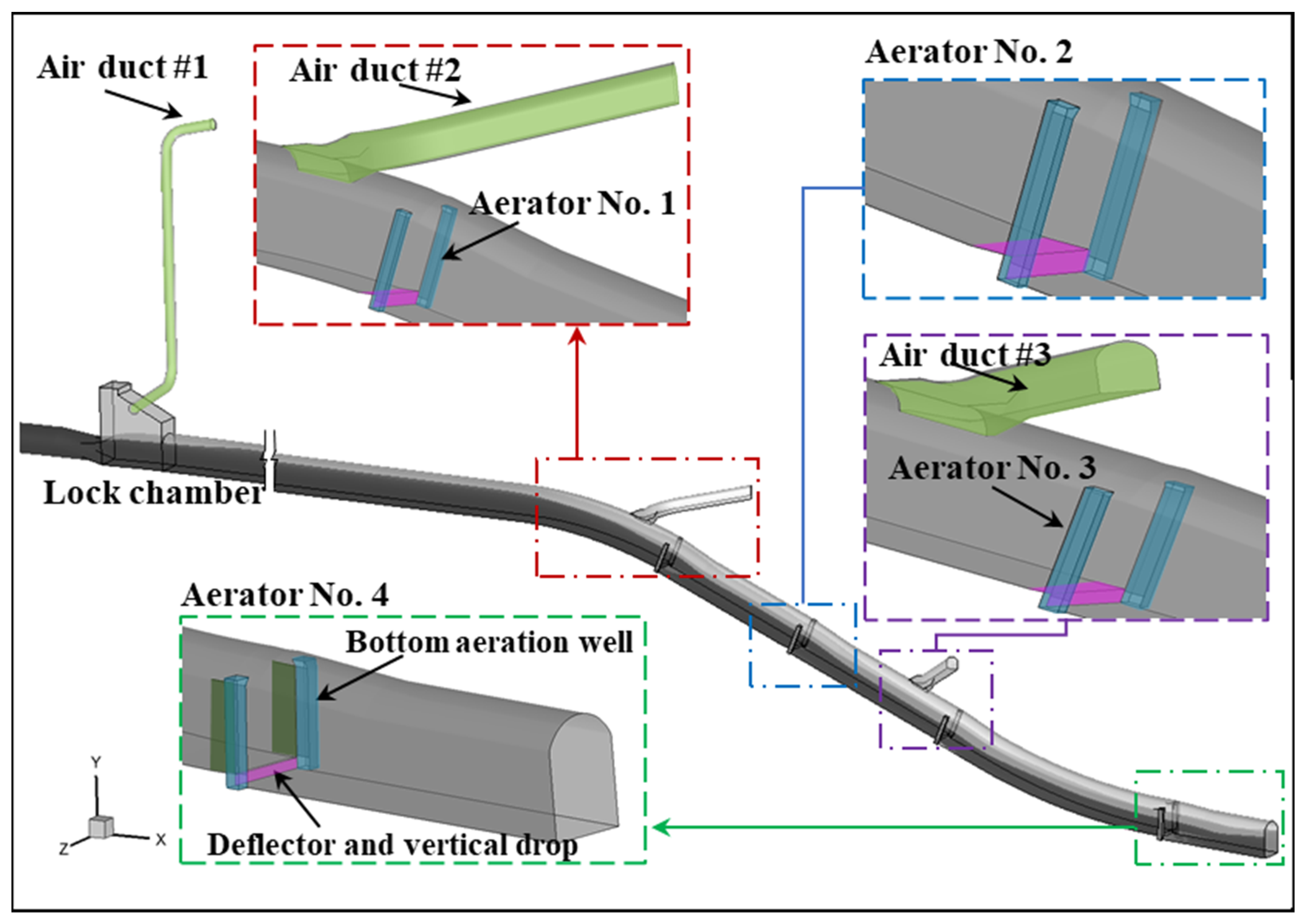
2.1. Prototype Observation Results

Jinping-I Dam, which is the highest dam in the world (305 m) by far, is located on the downstream of the Yalong River in southern China. The layout of the tunnel of Jinping-I project is depicted in Figure 1. The length downstream the lock chamber is about 800 m; the drop of bottom elevation is about 141 m; and the height and width of the cross-section are 17 m and 13 m, respectively. Three air ducts are installed between the tunnel gate and outlet. Four aeration devices are employed in the tunnel to prevent cavitation damage. Recently, prototype observation has been conducted to examine the ventilation capacities of air ducts and air entrainments of aerator. Prototype observation was conducted [23], and the results can be seen in

Table 1. Air demand and aeration concentration data from prototype observation.

Gate Opening Ratio	Flow Rate (m3/s)	Air Demand of Air Ducts (m3 s−1)			Average Aeration Concentration of Cross Section (%)
		Duct No. 1	Duct No. 2	Duct No. 3	Aerator No. 2	Aerator No. 4
25%	793	933.59	1402.13	892.08	27.79	32.19
50%	1460	1258.51	1805.52	1119.53	20.72	27.00
75%	2140	1543.3	2161.08	1495.33	17.35	22.11
100%	3220	1313.09	2097.1	1812.71	12.57	16.10

. The gate opening percentages are 25%, 50%, 75% and 100%.

2.2. Two-Fluid Model

2.2.1. Basic Equations

The classical Eulerian equations for both phases are solved:

$$\frac{\partial }{\partial t}\left({\rho }_k{\alpha }_k\right)+\nabla \cdot \left({\rho }_k{\alpha }_k{\mathbf{u}}_k\right)=0,$$

(1)

$$\frac{\partial }{\partial t}\left({\rho }_k{\alpha }_k{\mathbf{u}}_k\right)+\nabla \cdot \left({\rho }_k{\alpha }_k{\mathbf{u}}_k{\mathbf{u}}_k\right)=-\nabla \left({\alpha }_{k}p\right)+{\rho }_k{\alpha }_k\mathbf{g}+\nabla \cdot {\alpha }_k\left({\mathsf{\tau }}_k+{\mathsf{\tau }}_k^t\right)+{\mathbf{F}}_{km},$$

(2)

where k = W or A, which represents the water and air phase, respectively; $\rho$ is the density; $g$ is the gravitational acceleration; $\mathbf{u}$ is the vector of velocity; $p$ is the pressure; ${\mathsf{\tau }}_k$ and ${\mathsf{\tau }}_k^t$ are the stresses tensors of laminar and turbulent, respectively; ${\alpha }_k$ the volume fraction of each phase; and ${\mathbf{F}}_{km}$, which corresponds to the interaction forces between air and water, is the interphase momentum transfer per unit volume.

2.2.2. Interaction Forces

The interaction forces ${\mathbf{F}}_{km}$ consist of the added mass force ${\mathbf{F}}_{\mathrm{VM}}$, the lift forces ${\mathbf{F}}_{\mathrm{L}}$, and the drag force ${\mathbf{F}}_{\mathrm{D}}$. According to the previous study [24], the most important force is ${\mathrm{F}}_{\mathrm{D}}$:

$${\mathbf{F}}_{\mathrm{D}}=K_{\mathrm{D}}\left({\mathbf{u}}_{\mathrm{W}}-{\mathbf{u}}_{\mathrm{A}}\right)=\frac{{\rho }_{\mathrm{A}}f}{6{\tau }_{\mathrm{A}}}{d}_{\mathrm{A}}{A}_{\mathrm{I}}\left({\mathbf{u}}_{\mathrm{W}}-{\mathbf{u}}_{\mathrm{A}}\right),$$

(3)

where $K_{\mathrm{D}}$ is the interphase exchange coefficients; ${\tau }_{\mathrm{A}}=\left({\rho }_{\mathrm{A}}{d}_{\mathrm{A}}^2\right)/\left(18{\mu }_{\mathrm{W}}\right)$ is the particulate relaxation time; $A_{\mathrm{I}}={6{\alpha }_{\mathrm{A}}{\alpha }_{\mathrm{W}}/d}_{\mathrm{A}}$ is the interfacial area concentration, where $d_{\mathrm{A}}$ is the bubble diameter; and $f$ is the drag function.

For the model of Schiller and Naumann [25]:

$$f=\frac{C_{\mathrm{D}}\mathrm{Re}}{24},$$

(4)

where

$$C_{\mathrm{D}}=\left\{\begin{array}{l}24\left(1+0.15{\mathrm{Re}}^{0.687}\right)/\mathrm{Re},\mathrm{Re}\le 1000\\ 0.44 ,\mathrm{Re}>1000\end{array}\right.,$$

(5)

and Re is the relative Reynolds number:

$$\mathrm{Re}={\rho }_{\mathrm{W}}\left|{\mathbf{u}}_{\mathrm{W}}-{\mathbf{u}}_{\mathrm{A}}\right|d_{\mathrm{A}}/{\mu }_{\mathrm{W}},$$

(6)

For the symmetric model, the density and the viscosity in Equations (3)–(6) are calculated from volume-averaged properties [25]:

$${\rho }_{\mathrm{WA}}={\alpha }_{\mathrm{W}}{\rho }_{\mathrm{W}}+{\alpha }_{\mathrm{A}}{\rho }_{\mathrm{A}},$$

(7)

$${\mu }_{\mathrm{WA}}={\alpha }_{\mathrm{W}}{\mu }_{\mathrm{W}}+{\alpha }_{\mathrm{A}}{\mu }_{\mathrm{A}},$$

(8)

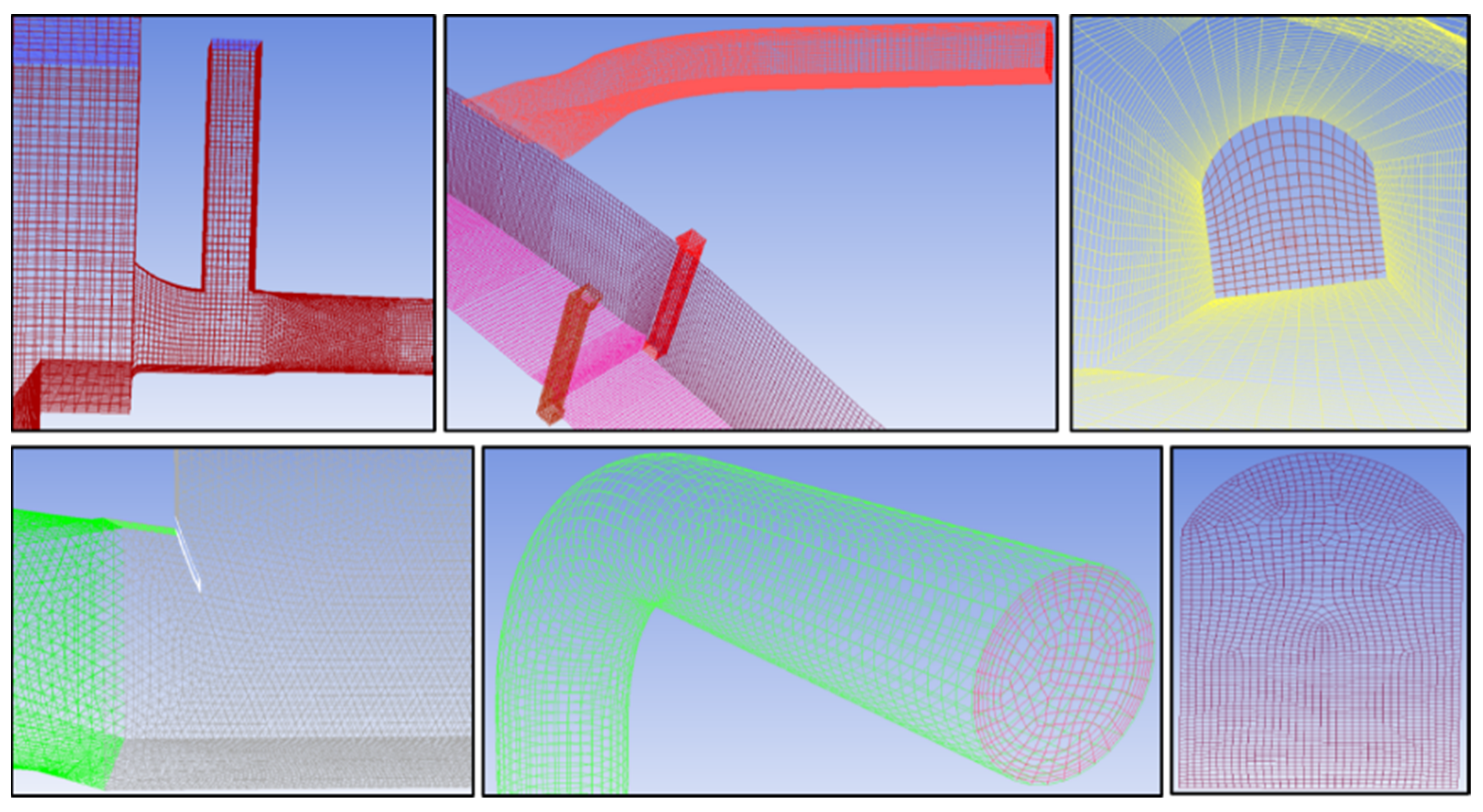
2.2.3. CFD Model Setup

A 3D mesh geometric model was established. The model starts from 50 m upstream of tunnel inlet to tunnel outlet, including the reservoir, pressurized tunnel, non-pressurized tunnel, air ducts no. 1 to no. 3 and aerator no. 1 to no. 4. The mesh is generated by the ICEM-CFD software in ANSYS15.0. As can be seen in Figure 2, the hexahedral grid is mainly used. The mesh refinements are carried out for the key parts including the aerators and air ducts. Furthermore, three sets of meshes for the 100% gate opening ratio are generated. The cell counts are 720,000, 2.03 million, and 3.23 million, and the corresponding equivalent grid sizes are 0.9816 m, 0.6940 m, and 0.5947 m, respectively.

Under the Euler–Euler framework, water phase is set as the primary phase (or continuous phase), while air phase is set as the secondary phase (or dispersed phase). The inlet boundary of reservoir is set as pressure inlet with a triangular distribution of hydrostatic pressure. The pressure value of this inlet is realized by the DEFINE_PROFILE macro in the User-Defined-Function interface of the commercial solver Fluent 15.0. The pressure boundary condition of tunnel outlet and other air inlet are set as fix-value with the atmosphere pressure (0 Pa). The tunnel walls are all set as no-slip wall boundary with roughness height of 0.001 m. To speed up the calculation, the initial volume fraction of water is set as 1 for the reservoir and pressurized tunnel.

3. Results

3.1. Verification

3.1.1. Grid Convergence

In the commercial solver Fluent 15.0, the continuous fluid is divided into a finite number of control bodies by the grid, and the hydrodynamic equations are solved discretely in these control bodies by the finite volume method (FVM). Therefore, it must be verified that the resolution of the mesh is sufficient to describe the movement of the fluid and the errors caused by the spatial discretization of the fluid are within an acceptable range. As can be seen in

Table 2. Examination of grid convergence.

	Air Duct No. 1			Air Duct No. 2			Air Duct No. 3
Grid parameter	Cell counts: 323 w; 203 w; 72 w Equivalent size h: 0.5947; 0.6940; 0.9816
	r21 = 1.1669; r32 = 1.4145
Air velocity (m/s)	69.12	70.37	77.97	66.54	67.53	73.31	57.78	58.37	63.36
φext	67.5259			65.2104			57.2601
ea	1.81%			1.49%			1.02%
eext	2.36%			2.04%			0.91%
GCIfine	2.88%			2.50%			1.12%

, the grid convergence method (GCI) [26] was applied to analyze the discretization error of air velocity of three air duct. The extrapolated values ${\phi }_{\mathrm{ext}}$, approximate relative error $e_a$, extrapolated relative error $e_{\mathrm{ext}}$, and the fine-grid convergence index ${\mathrm{GCI}}_{\mathrm{fine}}$ are listed in the table. The maximum ${\mathrm{GCI}}_{\mathrm{fine}}$ was 2.88%. Therefore, the discretization error was within the acceptable range and the mesh with 2.03 million grids was used in the following analysis.

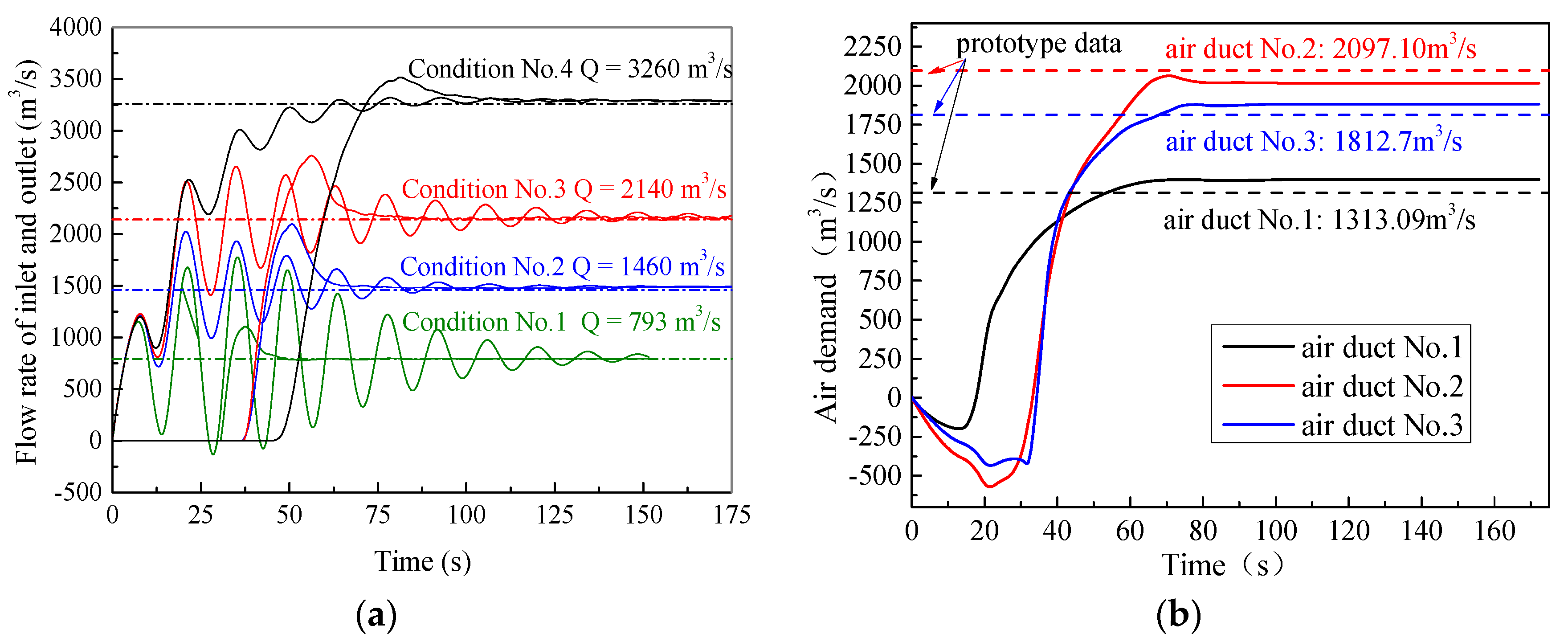
3.1.2. Time Independence

In consideration of convergence of the calculation process, the transient computation was used to approximate the steady state. Therefore, the sample convergence trends were documented for critically important variables. As can be seen in Figure 3, the inlet and outlet flow rate of water under four conditions in Table 1 all converged to a constant after about 150 s, and the air velocity of three air ducts converged to a constant after about 80 s. Accordingly, the analysis in this paper was based on these convergent values.

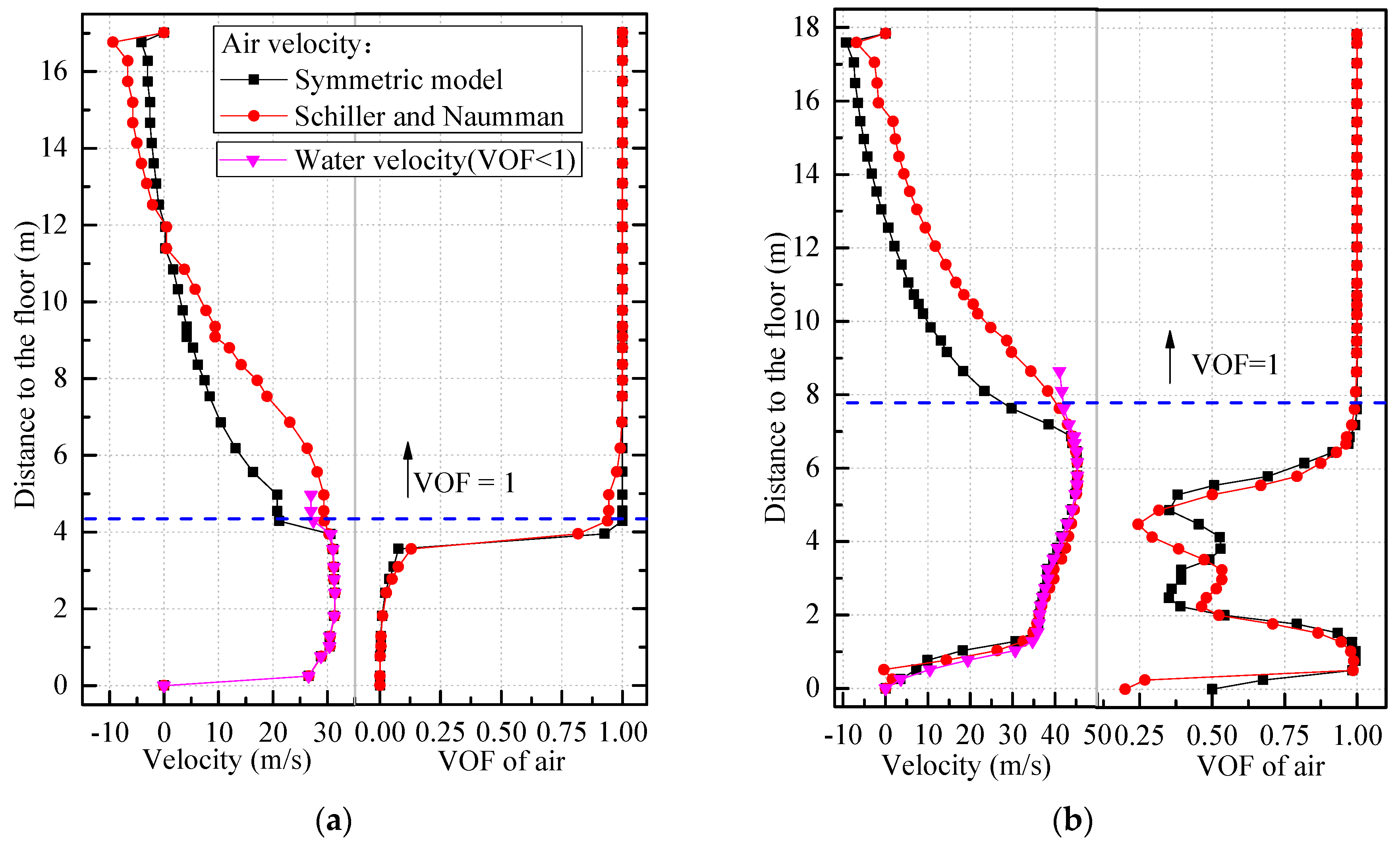
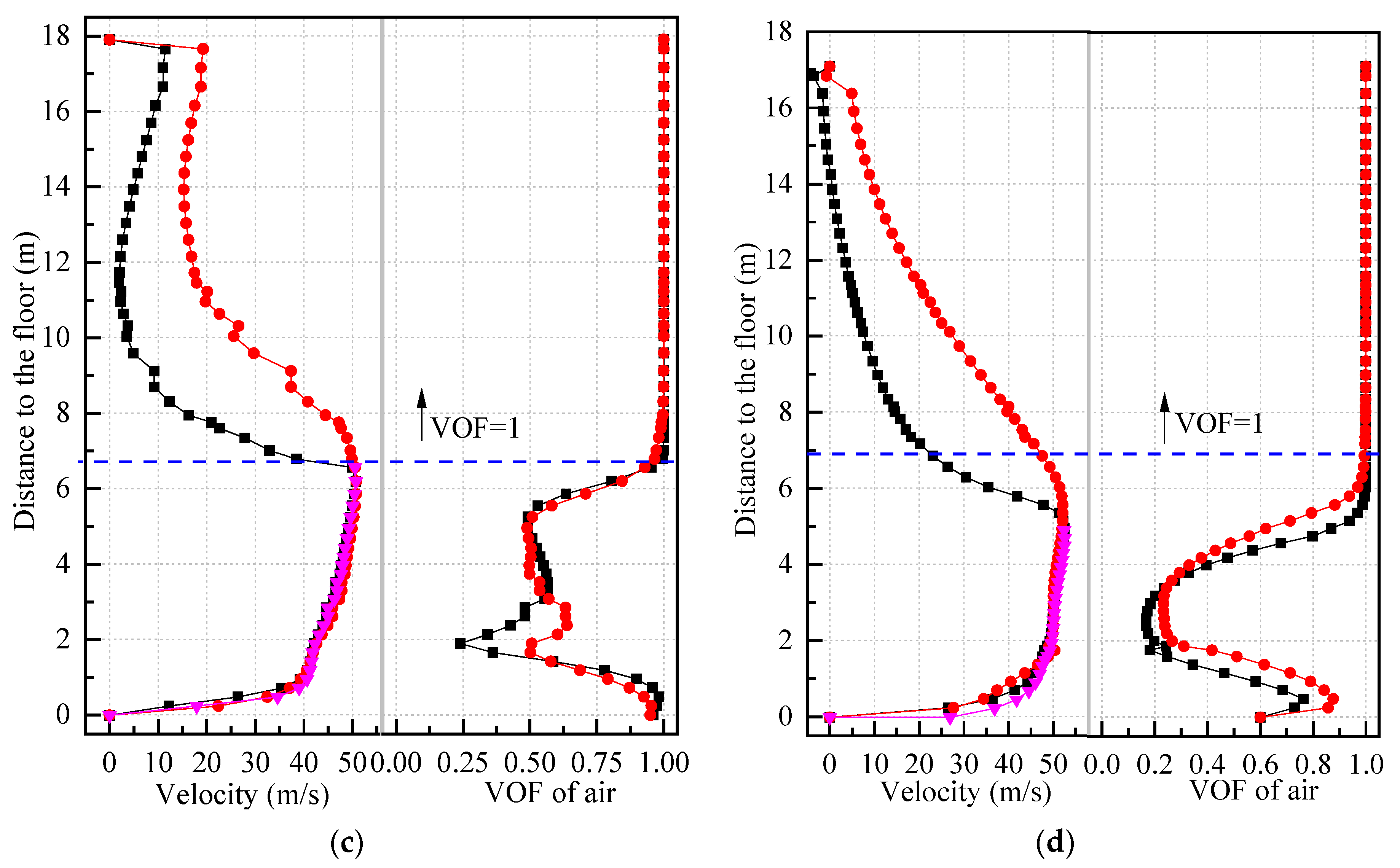
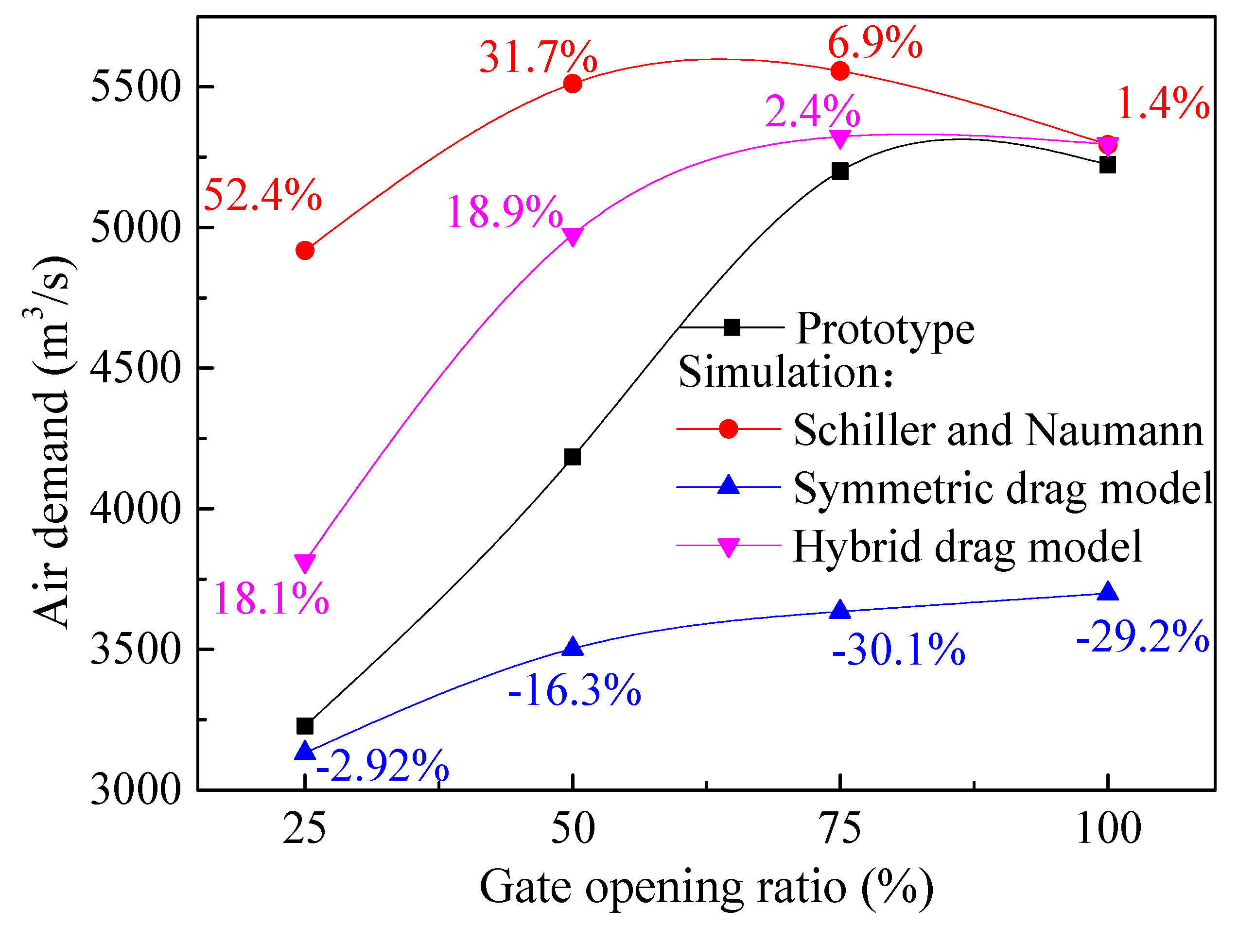
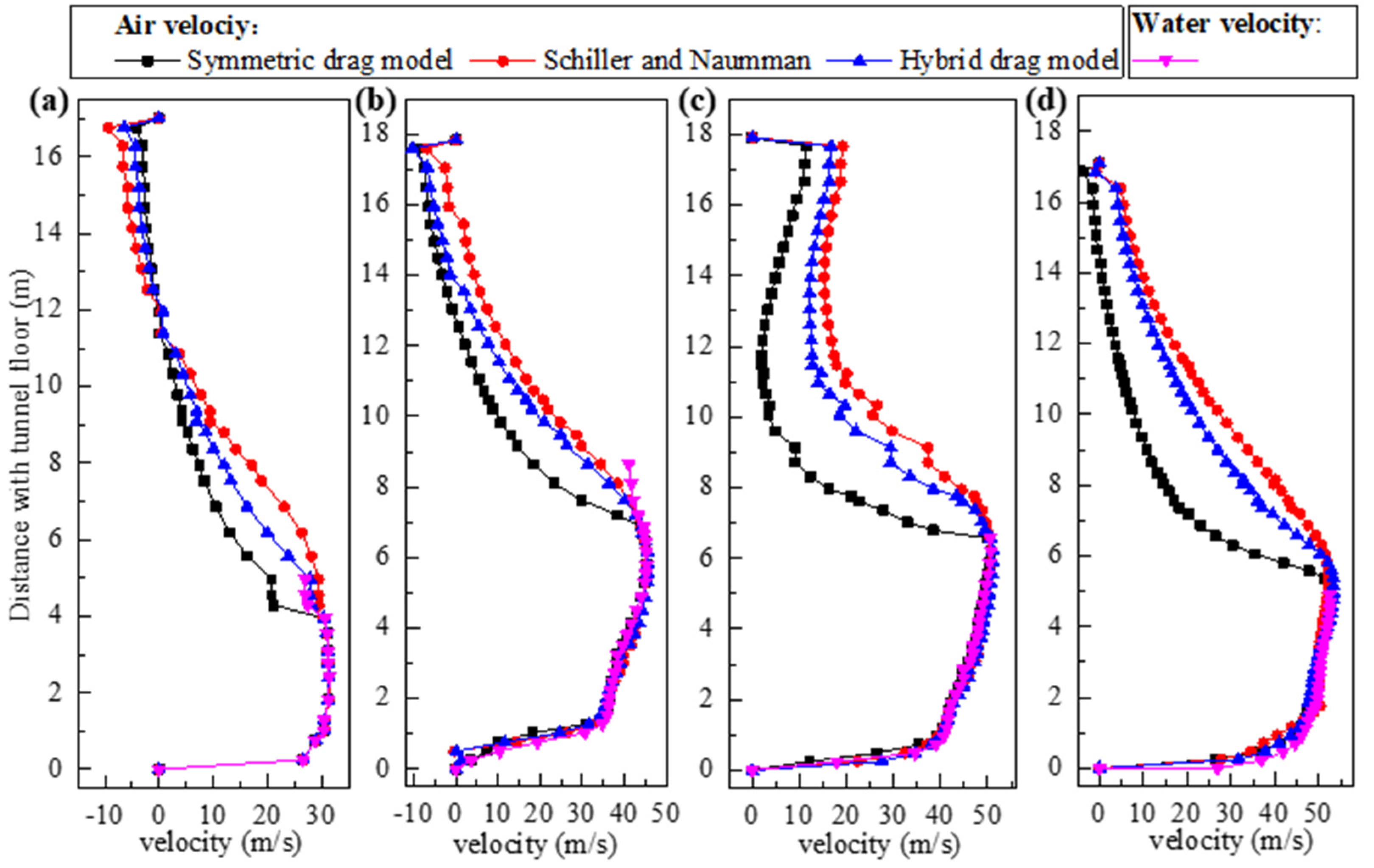
3.1.3. Air Demand and Velocity Profiles

As can be seen in Figure 4, the results of numerical simulation were compared to the prototype observation. The variation trend of air demand with gate opening obtained by numerical simulation was the same as that obtained by prototype observation. However, the results based on the Schiller and Naumann drag model were closer to the prototype data for large gate opening percentage, while the results based on the symmetric drag model were closer to the prototype data for small gate opening percentage.

In order to reveal the difference between the drag models, several typical sections were selected. Water velocity, air velocity, and air volume fraction ${\alpha }_a$ on the center line of these sections were extracted. As the water velocity from different drag models showed little discrepancy, only one profile for water velocity was plotted on every subfigure. In Figure 5, the profiles of air velocity in the location where ${\alpha }_a<1$ was close to the water velocity. This indicates that in the calculation of this paper, whether the Schiller and Naumann model or the Symmetric model was adopted, the distribution of air velocity in the water body would eventually be consistent with the profile of water velocity. However, near the air–water interface where ${\alpha }_a$ transforms from ${\alpha }_a<1$ to ${\alpha }_a=1$, the difference of the air velocity profile calculated from two models appeared. The air velocity calculated by the Symmetric model was obviously distorted here, and the large gradient resulted in a suddenly decrease of air velocity. The results of the symmetric drag model are generally smaller than those of the Schiller and Naumann models. Nevertheless, it is necessary to provide a more proper drag model since it has a great influence on the calculation of air demand of a spillway tunnel.

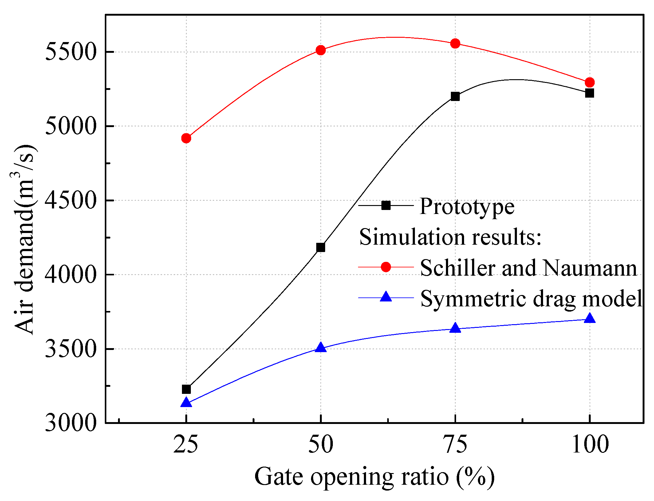
3.1.4. Improvement of the Drag Model

As can be seen in Figure 6, the gate panel and its bottom boundary were able to strongly disturb the water surface. As the gate opening percentage became larger, this effect waned. Obviously, when the gate opening is small, the drag effect of the free surface will be reduced because it is strongly disturbed and broken. In this case, the following features of airflow were poor, and thus the result of the symmetric model was more reasonable. On the contrary, when the gate was totally open, the drag effect of water on the air was stronger because the surface of the water was not disturbed and maintained better integrity. In this case, the following features of airflow were good, and therefore the result of the Schiller and Naumann model was more reasonable. Furthermore, although the disturbance effect of the gate may vanish far downstream from the gate, the air entrainment by forced-aeration or self-aeration in the tunnel will also destroy the continuity of water bodies, especially for the condition where gate opening percentage or water flow rate is small.

Here, a hybrid drag model was proposed on the basis of a parameter related to the gate opening to integrate the Schiller and Naumann model and symmetric model by a blending function:

$$K_{D,hyb}=\left(1-{\epsilon }^2\right)K_{D,sym}+{\epsilon }^2{K}_{D,s-n},$$

(9)

where $K_{D,hyb}$ are the interphase exchange coefficients of hybrid drag model, $K_{D,sym}$ are the coefficients calculated by the symmetric model, $K_{D,s-n}$ are the coefficients calculated by the Schiller and Naumann model, and $\epsilon$ is the percentage of gate opening. In this formula, when the gate is totally open, the hybrid model degenerates into the Schiller and Naumann model, while the hybrid model is closer to the symmetric model for small gate opening conditions. In the commercial solver Fluent 15.0, the interphase exchange coefficients $K_{D,hyb}$ in every cell can be calculated and applied to Equation (2) through the macro named DEFINE_EXCHANGE_PROPERTY.

The air demands of different gate-opening ratios were calculated on the basis of the hybrid drag model. As can be seen in Figure 7, the relative error of air demand prediction from the hybrid drag model was less than 20% for all conditions. Similarly, several typical cross-sections were selected. The water velocity, air velocity, and air volume fraction ${\alpha }_a$ on the center line of the sections were plotted in Figure 8. It is consistent with the previous analysis that the distribution of air velocity in the water body was eventually consistent with the profile of water velocity even for the hybrid drag model. Nevertheless, the air velocity profiles above the water of the hybrid model were between that of the Schiller and Neumman model and the symmetric model. It is suggested that the new model is more applicable for the prediction of air demand and air velocity profile under the complicated flow pattern in a high-head spillway tunnel. Therefore, the numerical simulation results based on the hybrid drag model are discussed further.

4. Discussion

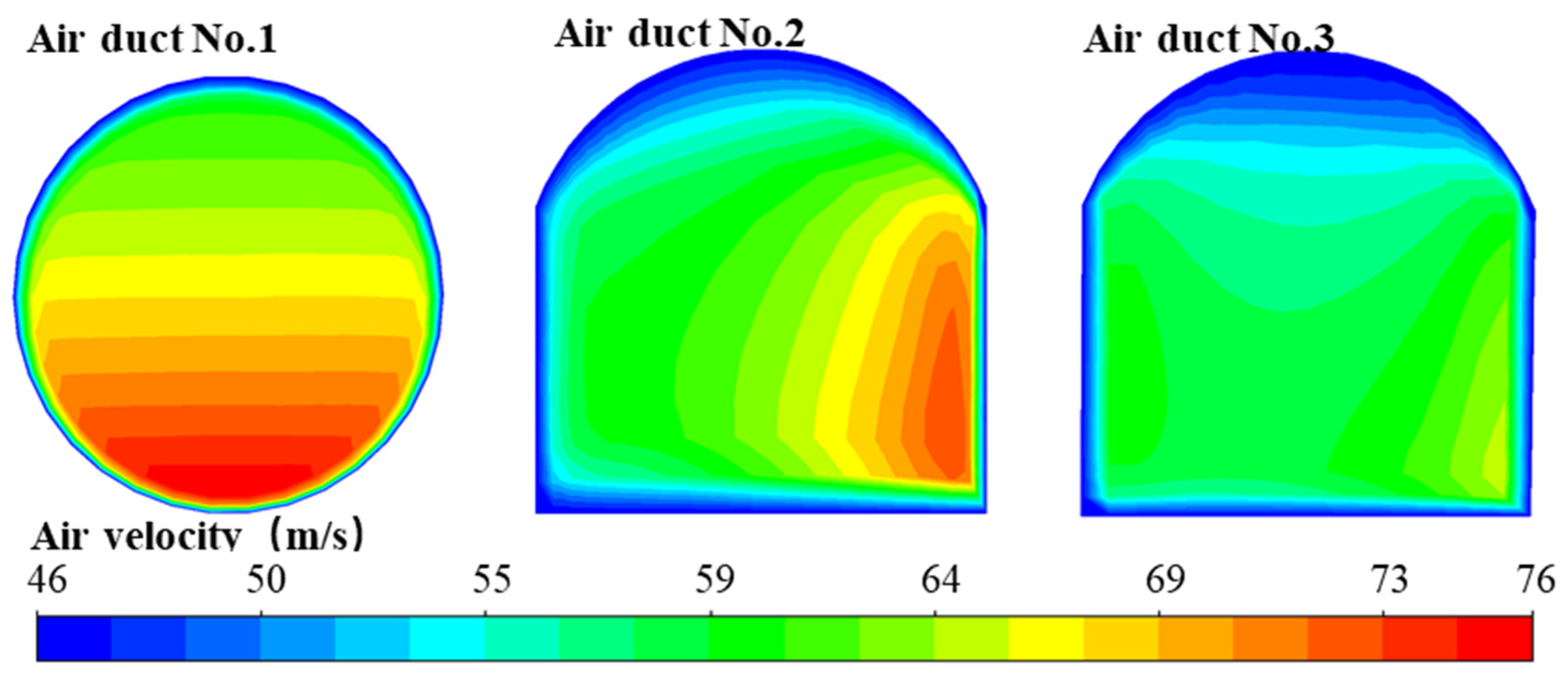
4.1. Air Velocity Distribution in Air Ducts

The contours of air velocity in the cross-sections of air ducts no. 1 to no. 3 under the 100% gate opening ratio can be seen in Figure 9. The air velocity of the air duct no. 1 decreased with the increase of the distance from the floor, and the maximum air velocity was about 76 m/s, while the minimum wind speed was about 46 m/s. The air velocity of the air ducts no. 2 and no. 3 were both larger at the downstream side wall, with the maximum air velocities of 73 m/s and 65 m/s, and the minimum air velocities of 49 m/s and 45 m/s, respectively. Near the wall of these ducts, the air flow was restricted by the wall boundary condition, resulting in a minimum air velocity.

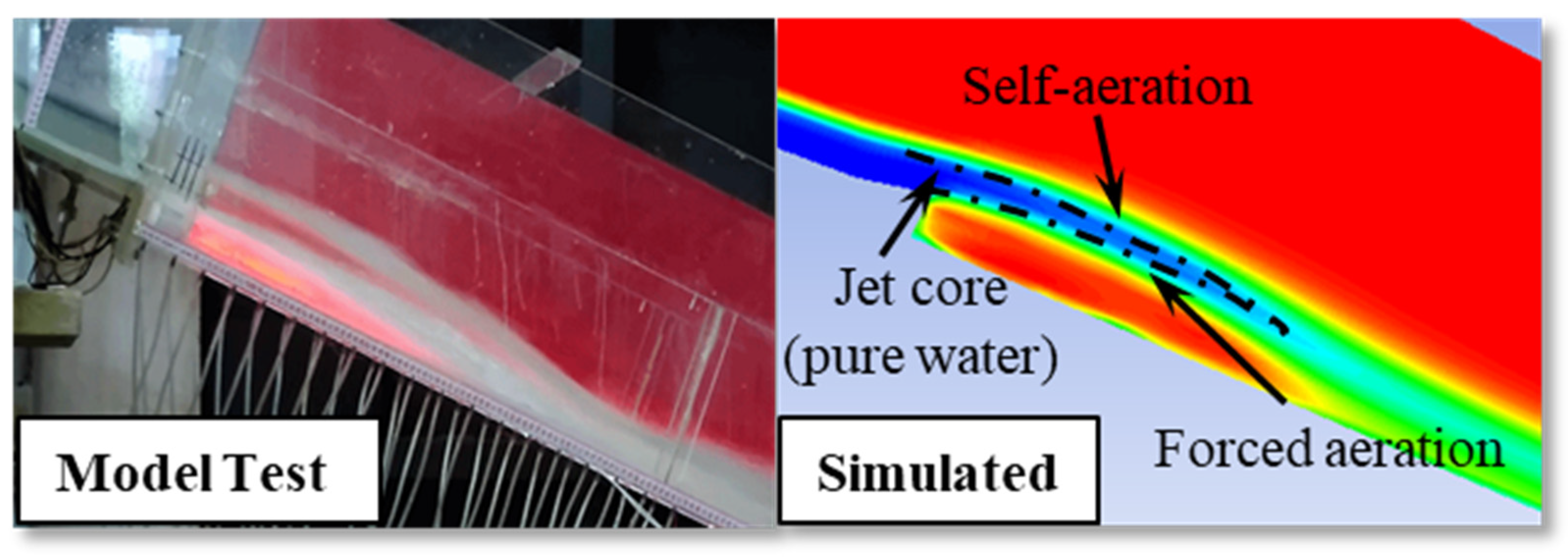
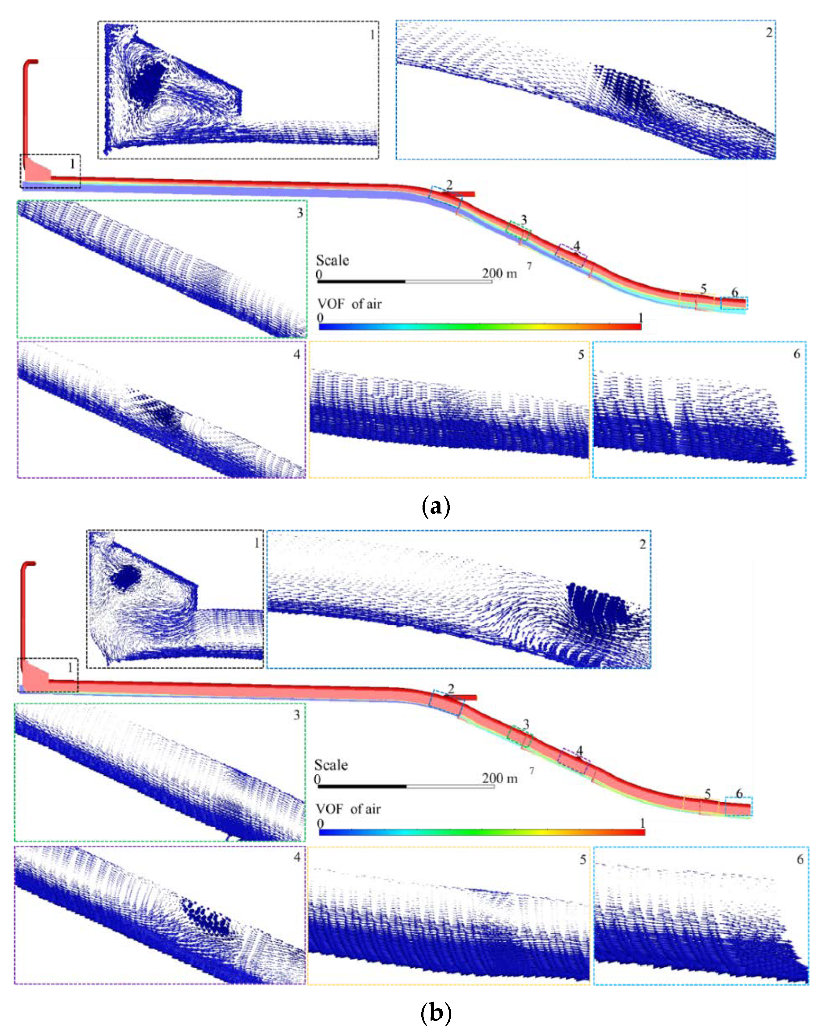
4.2. Water Tongue and Air Entrainment behind Aerators

As shown in Figure 10, the contour of air volume fraction of the water tongue behind the aerator no. 1 was compared to the model test result (Lian et al., 2017). It can be seen that the surface aeration region, forced aeration region, and the jet core with pure water were simulated successfully. The air entrainment and shape of water tongue were similar to that from the model test. In general, the Euler–Euler model based on the hybrid drag model was in accordance with the physical reality for the air–water two-phase flow in the spillway tunnel.

As shown in

Table 3. The average aeration concentration of cross-sections behind the aerators.

Gate Opening Ratio	Flow Rate (m3/s)	Aerator No. 2			Aerator No. 4
		Calculated	Prototype	Error (%)	Calculated	Prototype	Error (%)
25%	793	31.68%	27.79%	13.99	36.29%	32.19%	12.74
50%	1460	20.13%	20.72%	−2.83	24.49%	27.00%	−9.29
75%	2140	14.08%	17.35%	−18.82	17.63%	22.11%	−20.25
100%	3220	9.33%	12.57%	−25.80	11.54%	16.10%	−28.35

, the air entrainment quantities of the forced aerators were calculated for comparison with the prototype data. Restricted to prototype data, only the average aeration concentration of the cross-section behind the aerators no. 2 and no. 4 were listed. The average aeration concentration of the cross-section behind the aerators is defined as follows:

$$C_{average}=Q_{air}/\left(Q_{water}+Q_{air}\right),$$

(10)

where $Q_{air}$ is the air flux in the aeration well, and $Q_{water}$ is the water flow rate under the corresponding gate opening ratio. As can been seen, the maximum relative error was less than 30%, which means the aeration magnitude from numerical simulation was close to the prototype data. In addition, it is obvious that the quantities of air entrainment will not increase in an equal proportion with the increase of water flow rate.

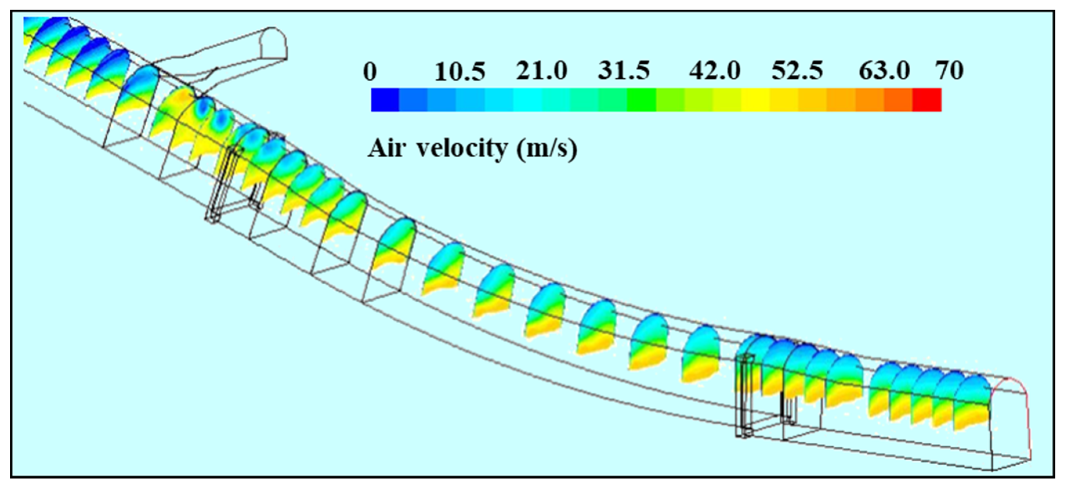
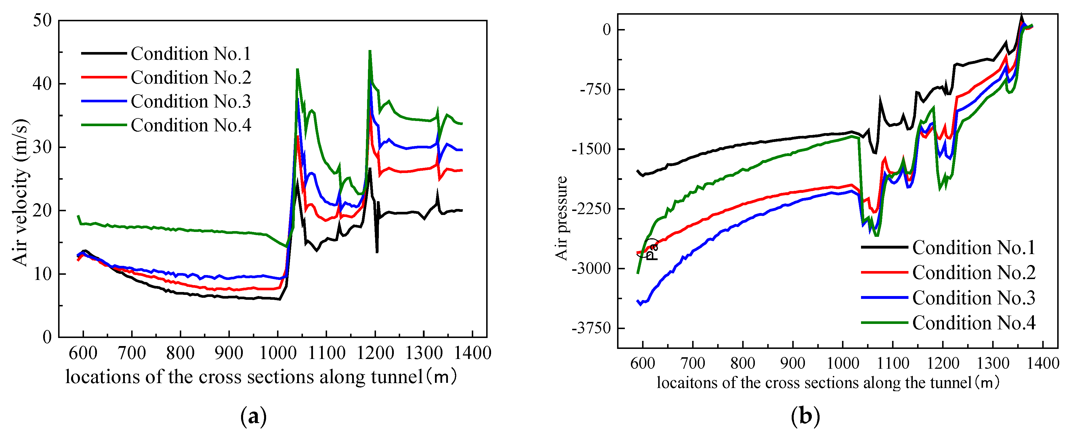
4.3. Air Velocity above Water in the Tunnel

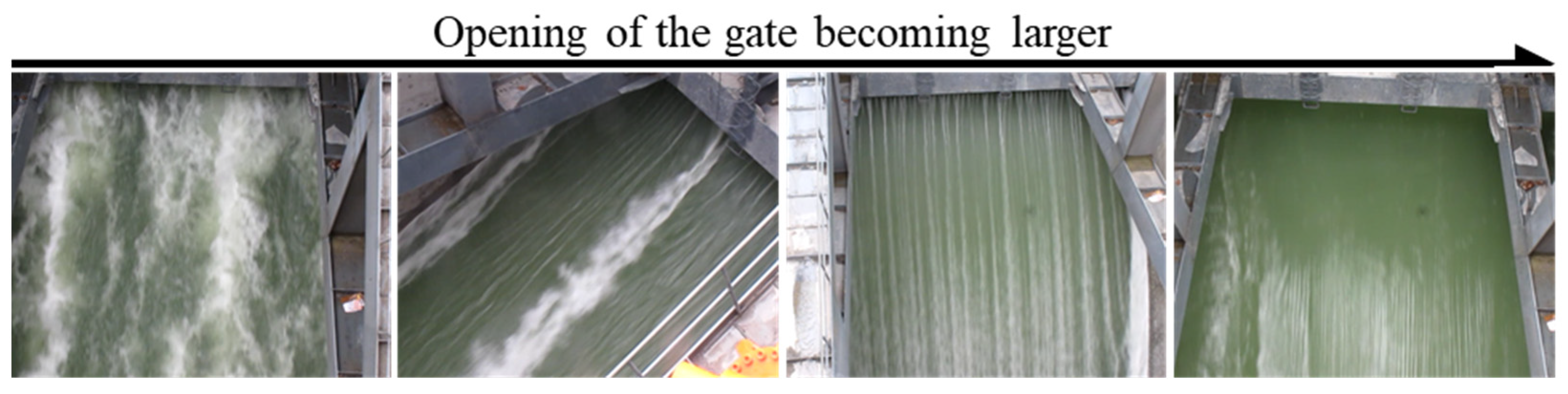
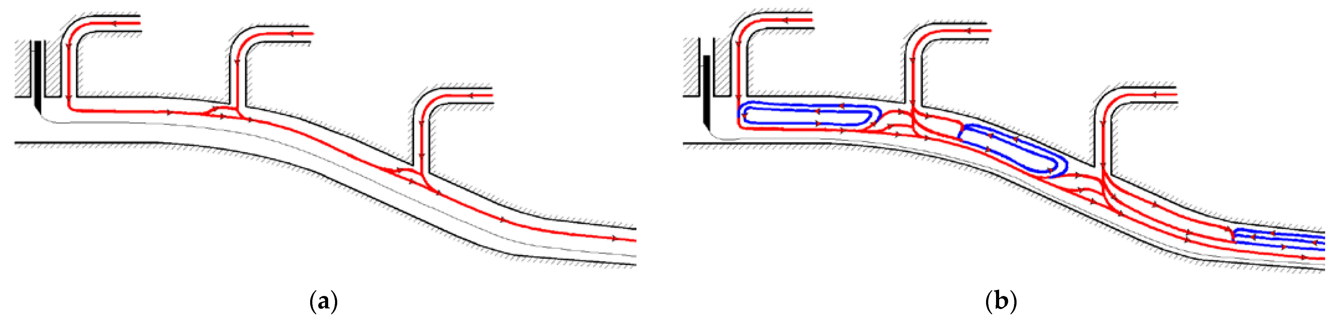
Several cross-sections along the flow direction in the tunnel were chosen to analyze the air flow characteristics in the tunnel. The region denoting the area residual of the tunnel was extracted from these cross-sections according to the volume fraction ${\alpha }_{\mathrm{a}}>0.5$. This allowed for the further analysis of air velocity, pressure, and other quantities that we care about in the tunnel. As can be seen in Figure 11, the contours of air velocity on this section showed the relative larger gradient on the direction perpendicular to the water surface than the direction perpendicular to the axial plane of the spillway tunnel. The maximum air velocity can be up to 50 m/s, while the minimum value can be close to zero.

As for the sectional average air velocity along flow direction in the tunnel shown in Figure 12a, due to the mass and momentum input of the air ducts, the air velocity increased suddenly at every intersection of the air ducts and the spillway tunnel. However, as the water flowed downstream, the water depth decreased. The increase of area residual resulted in the continuous decrease of average air velocity. Nevertheless, for the locations near the downstream of the gate where the water surface was disturbed intensively, the air entrainment of the water body led to the loss of air volume. The average air velocity at these sections decreased slightly.

As for the sectional average air pressure along flow direction shown in Figure 12b, due to the sudden increases of the air velocities at every intersection, the air pressure decreased suddenly according to Bernoulli’s law. Generally, the air pressure increased in the flow direction and eventually became atmospheric at the outlet of the tunnel. Furthermore, the air pressure under the 25% gate opening ratio was the largest, while the air pressure under the 75% gate opening ration rather than 100% was generally the smallest.

4.4. Flow Patterns

The flow pattern of the ventilation system of a spillway tunnel is very complex. The analysis of the vector field of air velocity is helpful in clarifying the reason for air demand difference under different gate opening ratios. It is also helpful to understand the balances between air ducts and residual space in a tunnel.

In the vector field of air velocity under the 100% gate opening ratio, it can be seen in Figure 13a that the flow pattern was relatively simple. The air flowing from air duct no. 1 generated several vortices in the gate chamber, and then flowed downstream to interconnect with the airflow flowing from air duct no. 2. Then, the confluence continued to flow downstream. Similarly, the airflow from the air duct no. 3 converged with the flow from upstream and flowed downstream until it is out of the tunnel. There was no obvious reverse flow in the residual space of the tunnel, and also no obvious airflow vortex.

In the vector field of air velocity under the 25% gate opening ratio (seen in Figure 13b), the flow pattern became more complex. On the downstream side of the chamber, there was obvious reverse airflow, which means part of the air flow in the chamber came from the downstream. Near the air duct no. 2 in the tunnel, part of the airflow from upstream converged with the air from air duct no. 2 and flowed downstream, while the other part was hindered and turned around to form a countercurrent, flowing upstream along the roof of the spillway tunnel. The airflow characteristics near the air duct no. 3 were similar to the characteristics near the air duct no. 2. Between the air duct no. 2 and no. 3, the airflow flowing downstream met the reverse flow from downstream, forming a local vortex. At the outlet, while the airflow was dragged out by the water flow, a small amount of air flowed back along the top of the tunnel. This part of airflow will finally form a vortex when it meets the airflow from upstream. The different flow patterns can be summarized as follows:

Pattern 1: as can be seen in Figure 14a, when the dragging capacity of water flow was sufficient, the air from the air duct was dragged downstream with the water flow, and there was little vortex in the residual space of the tunnel. In this case, the airflow field was simple, and the ventilation conditions were good.

Pattern 2: as can be seen in Figure 14b, when the dragging capacity of water was insufficient relative to the residual space of the tunnel, only part of the airflow can finally get out of the tunnel, while the rest part was locked between air ducts and outlet. The locked air formed self-circulation (or vortex) and occupied the residual space in the tunnel, which inhibited the process of air supply from the air ducts to the tunnel and finally reduced the air demand of the tunnel. The distribution area of the self-circulation was related to the equilibrium relationship between the dragging capacity of water flow and the size of residual space above water in a tunnel.

5. Conclusions

In this paper, the Euler–Euler two-phase flow model was applied in the numerical investigation of the air–water two-phase flow of the Jinping-I spillway tunnel.

The key factor that influences the prediction of air demand is the interphase exchange coefficients. The air velocity profile and air demand prediction based on different interphase exchange coefficients models, including the Schiller and Naumann model and the symmetric drag model, were analyzed. A hybrid drag model was proposed to improve the air demand prediction. The relative error of air demand prediction from the hybrid drag model was less than 18.9%, and the maximum relative error of average aeration concentrations of the cross-section behind the aerators was less than 28.35%, which means the results of numerical simulation can be verified by the prototype data.

On the basis of the new drag model, the air entrainment behind aerators, air velocity distribution in the air ducts, and the residual space of the tunnel were systematically analyzed. To summarize, the quantities of air entrainment increased in a smaller proportion with the increase of water flow rate. The air velocity along the flow direction in the tunnel decreased due to the increase of area residual, while the air velocity in the tunnel increased suddenly at every intersection of the air duct due to the mass and momentum.

Two flow patterns were finally summarized. In pattern 1, when the dragging capacity of water flow was sufficient, the airflow field was simple. In pattern 2, when the dragging capacity of water was insufficient relative to the residual space of the tunnel, part of the airflow was locked between the air ducts and outlet and occupied the residual space in the tunnel, inhibiting the process of air supply from the air ducts to the tunnel and finally reducing the air demand of the tunnel.

References

1. Safavi, K.; Zarrati, A.R.; Attari, J. Experimental study of air demand in high head gated tunnels. Proc. Inst. Civ. Eng. Water Manag. 2008, 161, 105–111. [Google Scholar] [CrossRef]
2. Lian, J.; Wang, X.; Ma, B.; Liu, D. Improvement to the sources selection to identify the low frequency noise induced by flood discharge. Mech. Syst. Signal Process. 2018, 110, 139–151. [Google Scholar] [CrossRef]
3. Lian, J.; Wang, X.; Liu, D. Air demand prediction and air ducts design optimization method for spillway tunnel. J. Hydraul. Res. 2020, 59, 448–461. [Google Scholar] [CrossRef]
4. Campbell, F.B.; Guyton, B. Air demand in gated outlet works. In Proceedings: Minnesota International Hydraulic Convention; ASCE: Reston, VA, USA, 2015. [Google Scholar]
5. U.S. Army Corps of Engineers (USACE). Air Demand Regulated Outlet Works; Hydraulic Design Criteria: New York, NY, USA, 1964. [Google Scholar]
6. Sharma, H.R. Air entrainment in high head gated conduits. J. Hydraul. Div. 1976, 102, 1629–1646. [Google Scholar] [CrossRef]
7. Speerli, J.; Hager, W.H. Air-water flow in bottom outlets. Can. J. Civ. Eng. 2000, 27, 454–462. [Google Scholar] [CrossRef]
8. Luo, H.Y. On the air intake problem of spillway tunnel. J. Hydraul. Eng. 1984, 8, 64–70. (In Chinese) [Google Scholar]
9. Chen, Z.H.; Huang, W.; Ye, S. A study of prototype law of air demand in flood control conduits. J. Nanjing Hydraul. Res. Inst. 1986, 1, 1–18. (In Chinese) [Google Scholar]
10. Deng, J. Investigation Report on the Air Demand in Flood Discharge Tunnel of High Dam Engineering; State Key Laboratory of Hydraulic and Mountain River Engineering, Sichuan University: Chengdu, China, 2017. (In Chinese) [Google Scholar]
11. Lian, J.; Ren, P.; Qi, C. A brief theoretical analysis on the ventilation characteristics of the multi-intake-well air supply system in a spillway tunnel. Appl. Sci. 2019, 9, 2793. [Google Scholar] [CrossRef] [Green Version]
12. Hohermuth, B.; Schmocker, L.; Boes, R.M. Air Demand of Low-Level Outlets for Large Dams. J. Hydraul. Eng. 2020, 146, 04020055. [Google Scholar] [CrossRef]
13. Wei, W.; Deng, J.; Xu, W. Numerical investigation of air demand by the free surface tunnel flows. J. Hydraul. Res. 2020, 59, 158–165. [Google Scholar] [CrossRef]
14. Yazdi, J.; Zarrati, A.R. An algorithm for calculating air demand in gated tunnels using 3D numerical model. J. Hydro-Environ. Res. 2011, 5, 3–13. [Google Scholar] [CrossRef]
15. Liu, T.; Yang, J. Three-dimensional Computations of Water–Air Flow in a Bottom Spillway During Gate Opening. Eng. Appl. Comput. Fluid Mech. 2014, 8, 104–115. [Google Scholar] [CrossRef] [Green Version]
16. Li, M.; Tian, Z. Influence of the ventilation area on the ventilation volume of the spillway tunnel and the wind field. Sichuan Water Power 2015, 34, 74–77. (In Chinese) [Google Scholar]
17. Salazar, F.; San-Mauro, J.; Celigueta, M.A. Air demand estimation in bottom outlets with the particle finite element method. Comput. Part. Mech. 2017, 4, 1–12. [Google Scholar] [CrossRef] [Green Version]
18. Yang, J.; Teng, P.; Xie, Q.; Li, S. Understanding Water Flows and Air Venting Features of Spillway—A Case Study. Water 2020, 12, 2106. [Google Scholar] [CrossRef]
19. Wardle, K.E.; Weller, H.G. Hybrid Multiphase CFD Solver for Coupled Dispersed/ Segregated Flows in Liquid-Liquid Extraction. Int. J. Chem. Eng. 2013, 2013, 128936. [Google Scholar] [CrossRef]
20. Ishii, M.; Mishima, K. Two-fluid model and hydrodynamic constitutive relations. Nucl. Eng. Des. 1984, 82, 107–126. [Google Scholar] [CrossRef]
21. Rehman, K.U.; Shatanawi, W.; Malik, M.Y. Heat transfer and double sampling of stratification phenomena in non-Newtonian liquid suspension: A comparative thermal analysis. Case Stud. Therm. Eng. 2022, 33, 101934. [Google Scholar] [CrossRef]
22. Munir, T.; Din, A.; Ullah, S.; Malik, M.Y.; Alqahtani, A.S. Discrete mass conservation and stability analysis of the ocean-atmosphere model with coupling conditions. J. Ocean Eng. Sci. 2022; in press. [Google Scholar] [CrossRef]
23. Lian, J.; Qi, C.; Liu, F.; Gou, W.; Pan, S.; Ouyang, Q. Air Entrainment and Air Demand in the Spillway Tunnel at the Jinping-I Dam. Appl. Sci. 2017, 7, 930. [Google Scholar] [CrossRef] [Green Version]
24. Simonnet, M.; Gentric, C.; Olmos, E.; Midoux, N. CFD simulation of the flow field in a bubble column reactor: Importance of the drag force formulation to describe regime transitions. Chem. Eng. Process. Process Intensif. 2008, 47, 1726–1737. [Google Scholar] [CrossRef]
25. ANSYS Inc. ANSYS FLUENT Theory Guide; ANSYS Inc.: Canonsburg, PA, USA, 2016. [Google Scholar]
26. Richardson, L.F. On the Approximate Arithmetical Solution by Finite Differences of Physical Problems Involving Differential Equations, with an Application to the Stresses in a Masonry Dam. Proc. R. Soc. Lond. 1910, 83, 335–336. [Google Scholar]
Figure 1. Layout of the spillway tunnel of Jinping-I project.
Applsci 12 04311 g001
Figure 2. Mesh of Jinping-I spillway tunnel model.
Applsci 12 04311 g002
Figure 3. The time independence of documented value: (a) flow rate of inlet and outlet; (b) air demand.
Applsci 12 04311 g003
Figure 4. Air demand comparison between prototype observation and numerical simulation.
Applsci 12 04311 g004
Figure 5. Water velocity and air volume fraction on the center line of typical sections (50% gate opening ratio) (a) downstream the gate, section marked 0 + 773.1 m; (b) downstream the aerator no. 2, section marked 1 + 141.90 m; (c) downstream the aerator no. 3, section marked 1 + 221.87 m; (d) downstream the aerator no. 4, section marked 1 + 360.52 m.
Applsci 12 04311 g005aApplsci 12 04311 g005b
Figure 6. The disturbance effect of gate.
Applsci 12 04311 g006
Figure 7. The comparison of air demand between prediction according to the different drag model and prototype data (the percentage on the lines represents relative prediction error).
Applsci 12 04311 g007
Figure 8. Water velocity and air volume fraction on the center line of typical sections (50% gate opening ratio) (a) downstream from the gate, section marked 0 + 773.1 m; (b) downstream from the aerator no. 2, section marked 1 + 141.90 m; (c) downstream from the aerator no. 3, section marked 1 + 221.87 m; (d) downstream from the aerator no. 4, section marked 1 + 360.52 m.
Applsci 12 04311 g008
Figure 9. Air velocity distribution in the cross-section of air ducts no. 1 to no. 3 under 100% gate opening ratio.
Applsci 12 04311 g009
Figure 10. Water tongue and air entrainment behind aerator no. 1.
Applsci 12 04311 g010
Figure 11. The regions of residual space along the tunnel and the contours of air velocity on it.
Applsci 12 04311 g011
Figure 12. The (a) average air velocity and (b) average air pressure over the cross-sections in the tunnel.
Applsci 12 04311 g012
Figure 13. Vectors of air velocity in the free space above water in the tunnel. (a) 100% gate opening ratio, (b) 25% gate opening ratio.
Applsci 12 04311 g013
Figure 14. Different flow patterns under different conditions: (a) pattern 1; (b) pattern 2.
Applsci 12 04311 g014