Solving Inverse Problems of Stationary Convection–Diffusion Equation Using the Radial Basis Function Method with Polyharmonic Polynomials

Abstract

In this article, the radial basis function method with polyharmonic polynomials for solving inverse problems of the stationary convection–diffusion equation is presented. We investigated the inverse problems in groundwater pollution problems for the multiply-connected domains containing a finite number of cavities. Using the given data on the part of the boundary with noises, we aim to recover the missing boundary observations, such as concentration on the remaining boundary or those of the cavities. Numerical solutions are approximated using polyharmonic polynomials instead of using the certain order of the polyharmonic radial basis function in the conventional polyharmonic spline at each source point. Additionally, highly accurate solutions can be obtained with the increase in the terms of the polyharmonic polynomials. Since the polyharmonic polynomials include only the radial functions. The proposed polyharmonic polynomials have the advantages of a simple mathematical expression, high precision, and easy implementation. The results depict that the proposed method could recover highly accurate solutions for inverse problems with cavities even with 5% noisy data. Moreover, the proposed method is meshless and collocation only such that we can solve the inverse problems with cavities with ease and efficiency.

1. Introduction

In recent years, numerical methods have been used extensively to simulate the movement of contaminants to groundwater [1,2]. Applications of groundwater pollution problems as well as inverse problems require accurate input data and parameters for solving the convection–diffusion equation [3]. However, the parameters are sometimes difficult to measure directly from the physical point of view. Meanwhile, measurement error and measurement uncertainty are often encountered. The inverse problems of the convection–diffusion equation involve the findings of the missing geometric shape, unknown physical parameters, and other conditions from historical observations [4,5].

Several numerical approaches have been successfully applied in the inverse problems for groundwater relative problems. The methods such as the model reduction technique, the differential evolution algorithm, and the collocation method have been used [6,7,8]. Identifying sources requires the solution of an inverse problem since this information has to be generally inferred from sparsely available measurements [9].

Inverse problems are often ill-posed, and the measurement uncertainty may enlarge numerical error exponentially in the solution [10,11]. To solve the ill-posed inverse problems, the meshless method, such as the Trefftz method and the radial basis function (RBF) method, may be a better alternative due to its meshless and high accuracy [12,13,14,15]. In order to model the backward inverse heat conduction problem, a meshless method based on the Trefftz formulation was presented [16]. Recently, the RBF method has become a promising numerical approach for solving direct problems [17,18,19,20]. Compared to the conventional RBF collocation method, the RBF method with the polyharmonic polynomials can obtain highly accurate solutions [21,22]. Accordingly, the attempt of using the collocation meshless method for solving inverse problems with cavities was made in this study.

The polyharmonic polynomials (PPs) are a series of polyharmonic RBFs, including even radial terms and natural logarithms [23]. Several inverse problems of convection–diffusion equation for the multiply-connected domains containing a finite number of cavities were investigated. Numerical solutions are approximated using polyharmonic RBFs instead of using the certain term of the polyharmonic RBF in the conventional polyharmonic spline at each source point. Additionally, highly accurate solutions can be obtained with the increase in the terms of polyharmonic polynomials. Additionally, examples in simply and multiply connected domains were carried out. A brief outline of the article is as follows: the description of the governing equation and boundary conditions are defined in Section 2; the mathematical formulation of the proposed method is introduced in Section 3; the convergence analysis is described in Section 4; several numerical examples are provided in Section 5; the disucssion is described in Section 6; and finally, conclusions are drawn in Section 7.

2. The Governing Equation

It is well known that the stationary groundwater pollution problem in porous media is governed by the convection–diffusion equation as follows [1,5]

$$Lu(\mathsf{x})=f(\mathsf{x}),\mathsf{x}\in \mathsf{\Omega },$$

(1)

where L is the differential operator, $L={\nabla }^2+\alpha \frac{\partial }{\partial x}+\beta \frac{\partial }{\partial y}+\gamma$; $u(\mathsf{x})$ is the variable of interest which usually is the concentration; x is the spatial coordinate, $x=(x,y)$; $f(\mathsf{x})$ is the given function; $\mathsf{\Omega }$ is the problem domain; $\nabla$ is the gradient; and $\alpha ,\beta$, and $\gamma$ are given functions. The boundary conditions are applied as follows:

$$B_{1}u(\mathsf{x})=g(\mathsf{x}),\mathsf{x}\in \partial {\mathsf{\Omega }}_1,$$

(2)

$$B_{2}u(\mathsf{x})=h(\mathsf{x}),\mathsf{x}\in \partial {\mathsf{\Omega }}_1,$$

(3)

where $\partial {\mathsf{\Omega }}_1$ is the boundary, $B_1$ and $B_2$ are boundary operators described as $B_1=1$ and $B_2=\partial /\partial \mathsf{n}$, $g(\mathsf{x})$ and $h(\mathsf{x})$ are the given functions, n is the outward normal vector described as $\mathsf{n}=(n_x,n_y^{})$, and $n_x$ and $n_y$ are the normal directions of the x and y axes, respectively.

The inverse problems for simply and multiply connected domains are displayed in Figure 1a,b, respectively. As illustrated in Figure 1a, the boundary includes $\partial {\mathsf{\Omega }}_1$ and $\partial {\mathsf{\Omega }}_2$, where $\partial {\mathsf{\Omega }}_1$ and $\partial {\mathsf{\Omega }}_2$ are the known and unknown boundaries, respectively. As depicted in Figure 1b, the boundary includes $\partial {\mathsf{\Omega }}_1$, $\partial {\mathsf{\Omega }}_2$, and $\partial {\mathsf{\Omega }}_3$, where $\partial {\mathsf{\Omega }}_3$ is the unknown boundary.

3. The Radial Basis Function

One of the commonly used polyharmonic RBF is [21,22,23]

$$\phi (r)=r_{}^{2k}\ln (r),k=1,2,3\cdots ,$$

(4)

where $\phi (r)$ is the basis function, r is the distance between points, written as $r=\left|\mathsf{x}-{\mathsf{x}}^s\right|$, x is the inner or boundary points, ${\mathsf{x}}^s$ is the source point, and k is the order which is a certain value. In this study, we propose polyharmonic polynomials (PPs), which are a series of polyharmonic RBFs at each center or source as follows:

$$\phi (r)={\displaystyle \sum _{k=1}^{M_N}{r}_{}^{2k}\ln (r),k=1,2,3\cdots }$$

(5)

where $M_N$ is the term of the PPs. The first derivative of Equation (5) for x and y yields the following:

$$\frac{\partial \phi (\mathsf{x})}{\partial x}\cong {\displaystyle \sum _{k=1}^{M_N}(x-x_{}^s)r_{}^{2k-2}[2k\ln (r)+1]},$$

(6)

$$\frac{\partial \phi (\mathsf{x})}{\partial y}\cong {\displaystyle \sum _{k=1}^{M_N}(y-y_{}^s)r_{}^{2k-2}[2k\ln (r)+1]},$$

(7)

where $x^s$ and $y^s$ are the x- and y-coordinates of the center point, respectively. The second derivative of Equation (5) yields the following:

$$\frac{{\partial }^2\phi (\mathsf{x})}{\partial x^2}\cong {\displaystyle \sum _{k=1}^{M_N}\left[{(x-x_{}^s)}^2{r}_{}^{2k-4}[(4k^2-4k)\ln (r)+4k-2]+r_{}^{2k-2}[2k\ln (r)+1]\right]}\mathrm{and}$$

(8)

$$\frac{{\partial }^2\phi (\mathsf{x})}{\partial y^2}\cong {\displaystyle \sum _{k=1}^{M_N}\left[{(y-y_{}^s)}^2{r}_{}^{2k-4}[(4k^2-4k)\ln (r)+4k-2]+r_{}^{2k-2}[2k\ln (r)+1]\right]}$$

(9)

Employing the PPs for the function approximation, we have:

$$u(\mathsf{x})\cong {\displaystyle \sum _{j=1}^{M_O}{\displaystyle \sum _{k=1}^{M_N}{a}_{j,k}}}{r}_j^{2k}\ln (r_j),$$

(10)

where $a_{j,k}$ is the unknown coefficient determined by collocation, $M_O$ is the total number of source points, $r_j$ is the radial distance at the jth source point, $r_j=\left|x-x_j^s\right|$, and $x_j^s$ is the jth source point described as $x_j^s=(x_j^s,y_j^s)$. Equation (10) is the function approximation that is built up by intruding the proposed PPs into the RBF. In order to satisfy the boundary conditions (as shown in Equations (2) and (3)), Equation (10) is then imposed at each boundary point. Therefore, we primarily adopt Equation (10) for collocating the boundary points in this study.

Inserting the aforementioned equations into Equation (1), the governing equation can be written as:

$$\begin{array}{l}{\displaystyle \sum _{j=1}^{M_O}{\displaystyle \sum _{k=1}^{M_N}{a}_{j,k}{r}_j^{2k-2}[4k^2\ln (r_j)+4k]}}+\alpha {\displaystyle \sum _{j=1}^{M_O}{\displaystyle \sum _{k=1}^{M_N}{a}_{j,k}(x-x_j^s)r_j^{2k-2}[2k\ln (r_j)+1]}}\\ +\beta {\displaystyle \sum _{j=1}^{M_O}{\displaystyle \sum _{k=1}^{M_N}{a}_{j,k}(y-y_j^s)r_j^{2k-2}[2k\ln (r_j)+1]}}+\gamma {\displaystyle \sum _{j=1}^{M_O}{\displaystyle \sum _{k=1}^{M_N}{a}_{j,k}{r}_j^{2k}\ln (r_j)}=f(\mathsf{x})}.\end{array}$$

(11)

Equation (11) is mainly utilized for the discretization of inner collocation points within the solution domain. Since the proposed PPs are not a solution to the stationary convection–diffusion equation, the inner points must be collocated inside the domain for the discretization. Thus, Equation (11) is mainly imposed to satisfy the governing equation (stationary convection–diffusion equation) at each inner point. By using Equation (11) and boundary data as shown in Equations (2) and (3), we obtained the following linear system:

$$Pa=Q,$$

(12)

in which P is an $n\times m$ matrix, where $m=M_O\times M_N$, $n=n_I+n_D+n_N$, $n_I$ is the inner collocation number, $n_D$ is the boundary point number for Dirichlet boundary, $n_N$ is the boundary point number for Neumann boundary, a is an $m\times 1$ vector that includes unknown coefficients described as $a={[a_1{a}_2\dots a_m]}^{\mathrm{T}}$, Q is an $n\times 1$ vector, n is the total number of points, and $a_1,a_2,\dots ,a_m$ are the unknown coefficients to be solved.

The input data with noises are considered as follows:

$$\widehat{g}(\mathsf{x})=g(\mathsf{x})\times (1+\delta \times rand)\mathrm{and}\widehat{h}(\mathsf{x})=h(\mathsf{x})\times (1+\delta \times rand),$$

(13)

where $\widehat{g}(x)$ and $\widehat{h}(x)$ are the input data with noises, rand is a random number ranging from −1 to 1, and $\delta$ is the noise level. The maximum absolute error (MAE) is

$$\mathrm{MAE}=\max \left|\widehat{u}\left({\mathsf{x}}_j\right)-u\left({\mathsf{x}}_j\right)\right|,1\le j\le n_t,$$

(14)

and the root mean square error (RMSE) is

$$\mathrm{RMSE}=\sqrt{{\displaystyle \sum _{j=1}^{n_t}{[\widehat{u}({\mathsf{x}}_j)-u({\mathsf{x}}_j)]}^2}/n_t},$$

(15)

where $n_t$ is the validation point number and $\widehat{u}(x_j)$ and $u\left(x_j\right)$ are the analytical and numerical solutions at the jth validation point, respectively. The validation points coincided with the inner points where Equation (11) is imposed.

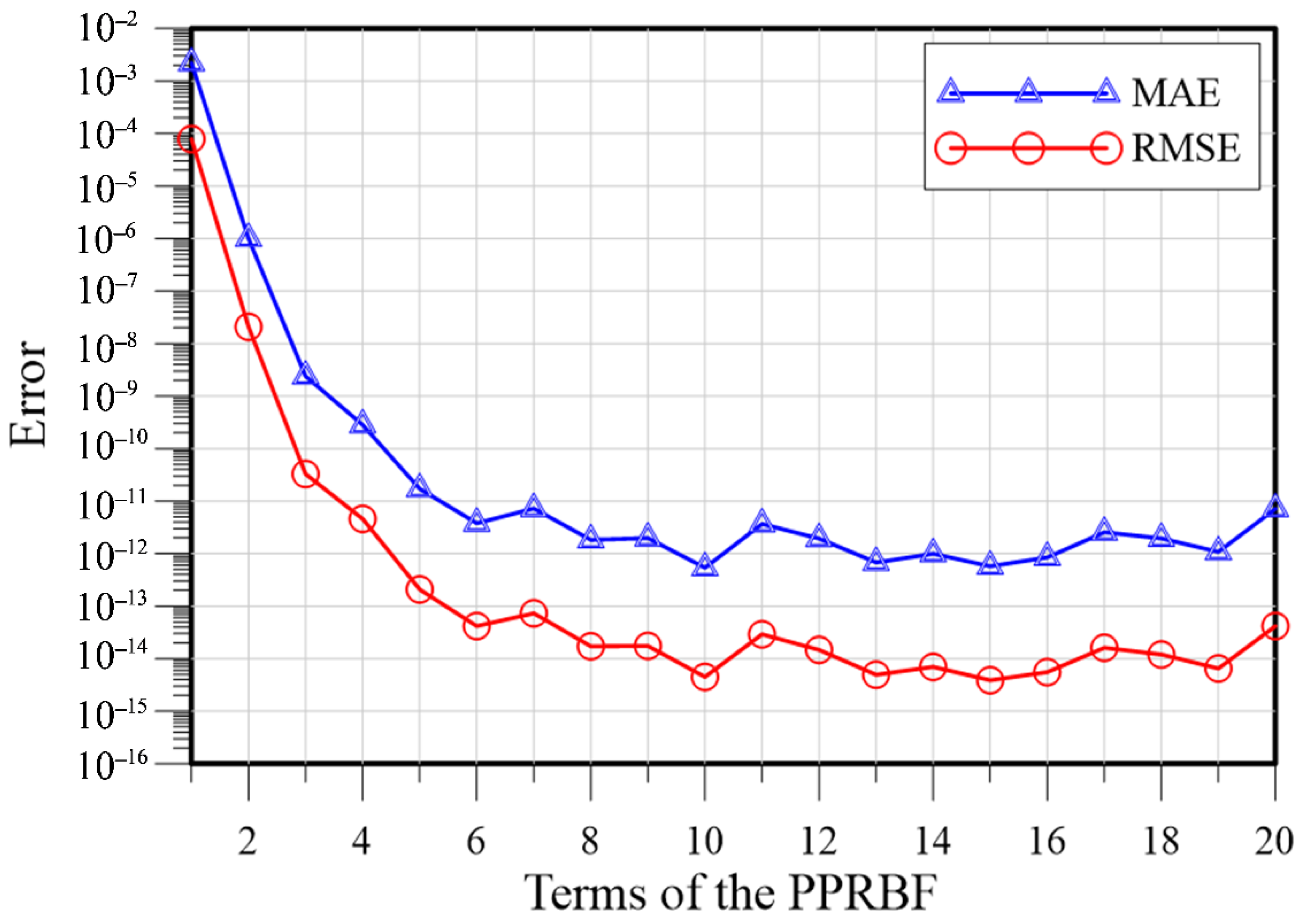
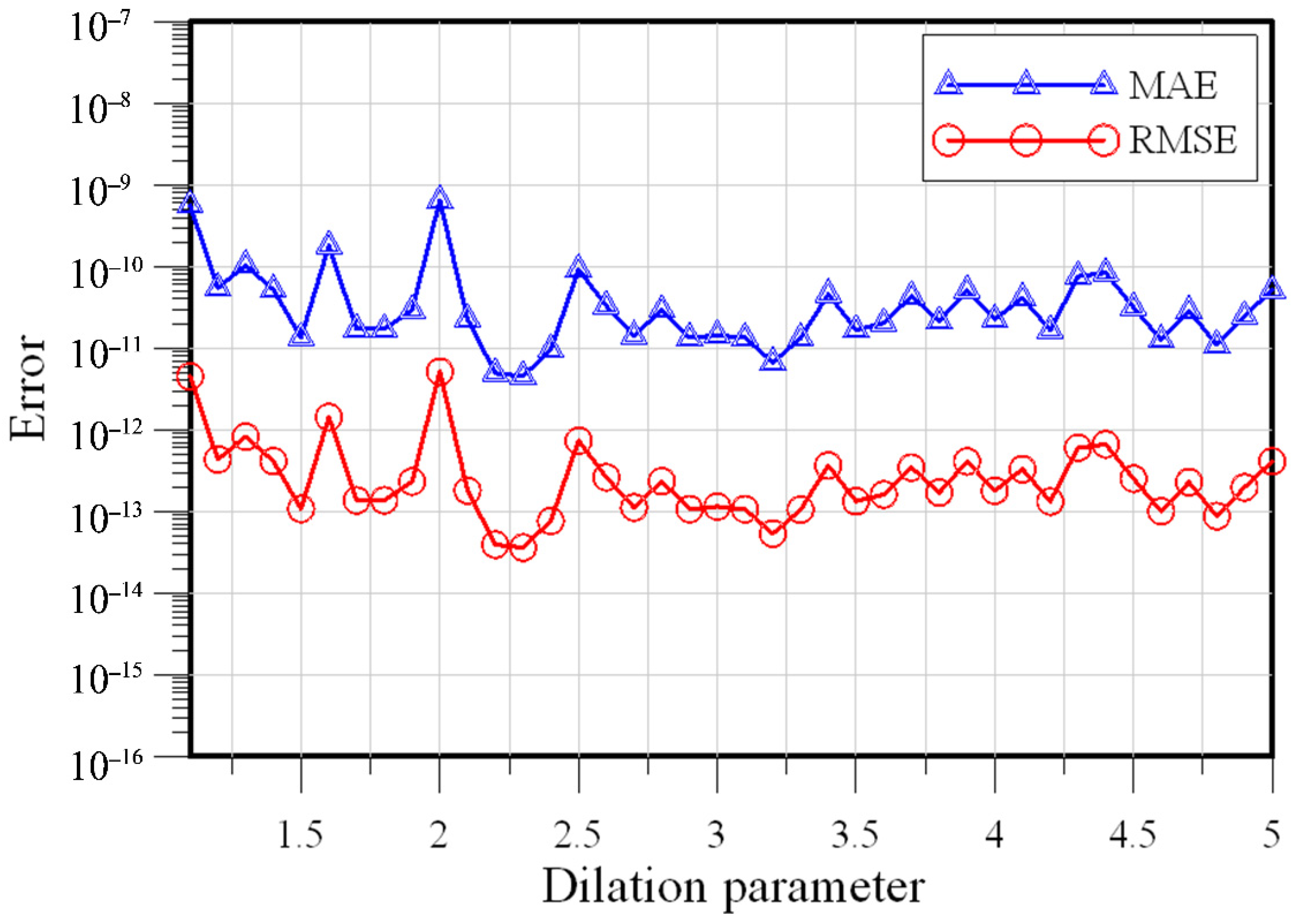
4. Validation of the Proposed RBF

A benchmark problem enclosed by a simply connected domain was adopted for the validation. We adopted the simplified form of Equation (1), which is the Laplace equation for the inverse problem for the validation as

$${\nabla }^{2}u(\mathsf{x})=0.$$

(16)

The boundary shape is

$$\begin{gathered} \partial \mathsf{\Omega }=\left\{(x,y)|x=\rho (\theta )\cos (\theta ),y=\rho (\theta )\sin (\theta ),0\le \theta \le 2\pi \omega \right\}, \\ \rho (\theta )=\sqrt[1/3]{\cos (3\theta )+\sqrt{2-{\sin }^2(3\theta )}}. \end{gathered}$$

(17)

The boundary conditions are expressed as follows:

$$B_{1}u(\mathsf{x})=g(\mathsf{x}),\mathsf{x}\in \partial {\mathsf{\Omega }}_1,$$

(18)

$$B_{2}u(\mathsf{x})=h(\mathsf{x}),\mathsf{x}\in \partial {\mathsf{\Omega }}_1.$$

(19)

The overspecified boundary conditions are assigned using the analytical solution:

$$u(\mathsf{x})=e^y\sin x+e^x\sin y.$$

(20)

The sources are placed outside the boundary using the equation.

$${\mathsf{x}}_j^s=\eta {\rho }_j^s\left(\cos {\theta }_j^s,\sin {\theta }_j^s\right),j=1,\dots ,M_O,$$

(21)

where $\eta$ is the dilation parameter, ${\rho }_j^s$ is the radius of the sources at the jth source point, and ${\theta }_j^s$ is the angle of the sources at the jth source point.

For obtaining better accuracy, the centers are often regarded as fictitious sources that are randomly scattered within the domain. In this study, we attempted to increase the accuracy by locating the sources in different ways. For investigating the accuracy, three different scenarios for locating the source points are considered, as illustrated in Figure 2. The first scenario is that the sources are randomly located inside the domain shown in Figure 2a. The second scenario is that the sources are simultaneously located within and outside the computational domain depicted in Figure 2b. The third scenario is that the sources are collocated outside the domain demonstrated in Figure 2c. The number of the source points for three different scenarios, as shown in Figure 2, is actually equal to investigating the accuracy of the proposed three collocation scenarios.

In this study, the convergence analysis for the number of source points is conducted to find the optimal number of source points. The results obtained demonstrate that promising numerical solutions can be achieved when the number of source points is greater than 300. Accordingly, the number of source points can then be determined. After determining the optimal number of source points based on the convergence analysis, another convergence analysis for the terms of the basis functions is then carried out to find the optimal terms of the basis functions, as shown in Figure 3. Figure 3 illustrates the RMSE of the three scenarios for locating the sources. As depicted in Figure 3, the third scenario exhibits higher accuracy in the order of 10⁻¹¹ than those of the first and the second scenarios. Accordingly, we may conclude that the sources collocated outside the domain are suggested for locating the sources. Figure 4 depicts the error versus the dilation parameter values for the third scenario. The MAE fluctuates from 10⁻⁷ to 10⁻¹¹, while the dilation parameter ranges from 1.1 to 5. Figure 5 illustrates the error versus the proportion of the accessible boundary. From Figure 5, the value of the accessible boundary to be 1 means that the entire set of boundary values is prescribed. Additionally, the accessible boundary to be 1 represents that the problem becomes a forward problem. For the forward problem, we found the solution within the domain similar to the boundary value problem in which the entire boundary values are given. On the other hand, the accessible boundary value less than 1 represents that the problem becomes an inverse problem. The inverse problems of the convection–diffusion equation involve the findings of the solution within the domain as well as missing boundary values. The results obtained show that both MAE and RMSE decrease with greater accessible boundary values.

Considering the given data polluted by random noise, the noise level is ranged from 10⁻² to 10⁻⁶.

Table 1. Errors of the proposed method with various noise levels.

Noise Level	$\mathit{\omega }=75\%$		$\mathit{\omega }=50\%$
	MAE	RMSE	MAE	RMSE
${10}^{-6}$	$2.57\times {10}^{-6}$	$5.00\times {10}^{-8}$	$8.43\times {10}^{-6}$	$8.67\times {10}^{-8}$
${10}^{-5}$	$2.58\times {10}^{-6}$	$5.54\times {10}^{-7}$	$3.62\times {10}^{-5}$	$7.77\times {10}^{-7}$
${10}^{-4}$	$4.69\times {10}^{-5}$	$1.01\times {10}^{-6}$	$7.74\times {10}^{-5}$	$1.66\times {10}^{-6}$
${10}^{-3}$	$8.10\times {10}^{-5}$	$1.74\times {10}^{-6}$	$7.67\times {10}^{-5}$	$1.65\times {10}^{-6}$
$0.01$	$2.40\times {10}^{-3}$	$5.21\times {10}^{-5}$	$3.20\times {10}^{-3}$	$6.91\times {10}^{-5}$
$0.02$	$2.90\times {10}^{-3}$	$6.28\times {10}^{-5}$	$5.20\times {10}^{-3}$	$1.12\times {10}^{-4}$
$0.03$	$6.90\times {10}^{-3}$	$1.49\times {10}^{-4}$	$7.20\times {10}^{-5}$	$1.55\times {10}^{-4}$

lists the error of the proposed method for the inverse problem where the percentages of the accessible boundary are $\omega =75\%$ and $\omega =50\%$. Thus, accurate results can be achieved even with input data polluted by noise. Figure 6 demonstrates the comparison of results for solving inverse problems. Results computed using the proposed method are agreed with the exact solution.

5. Numerical Examples

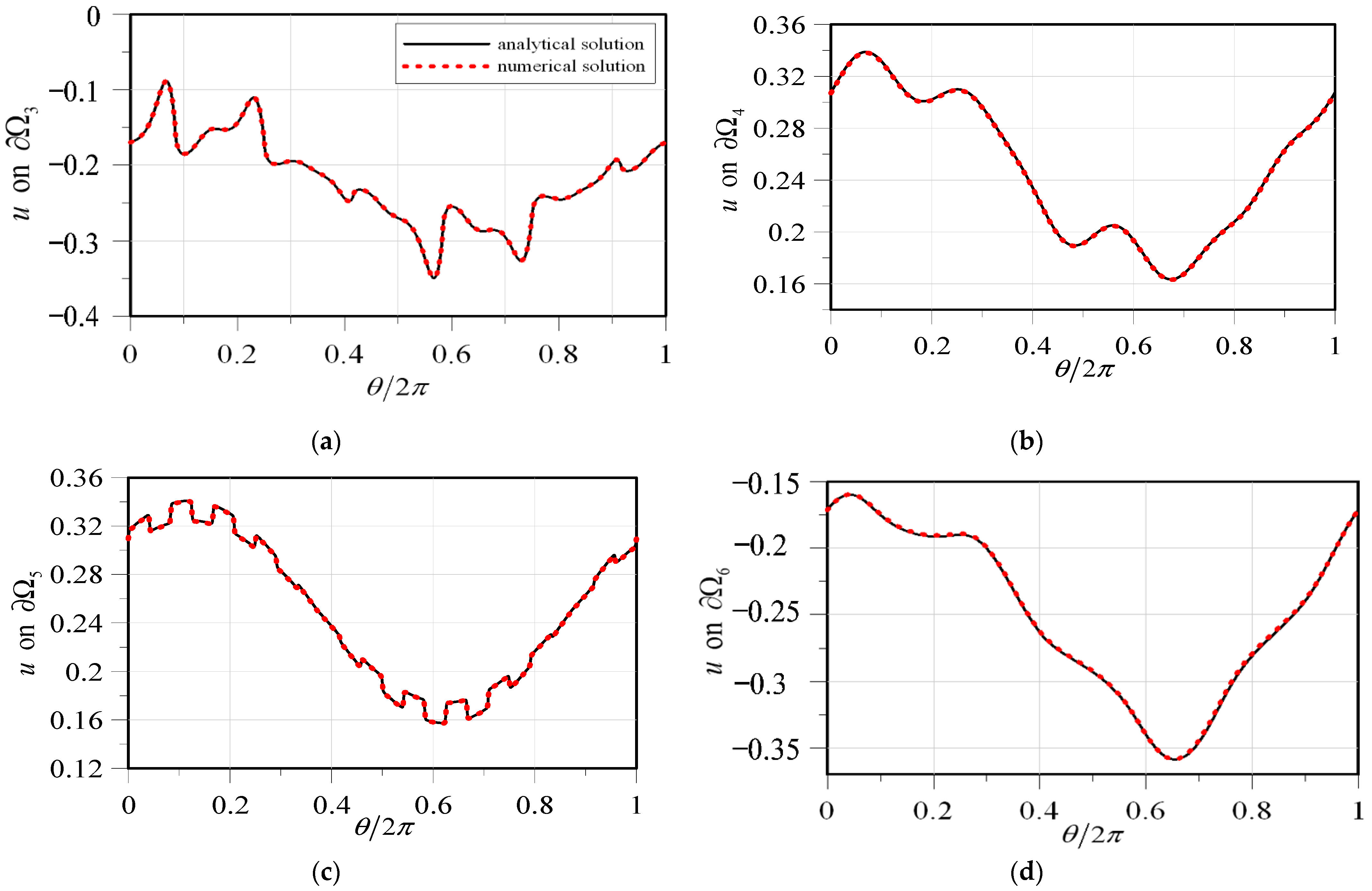
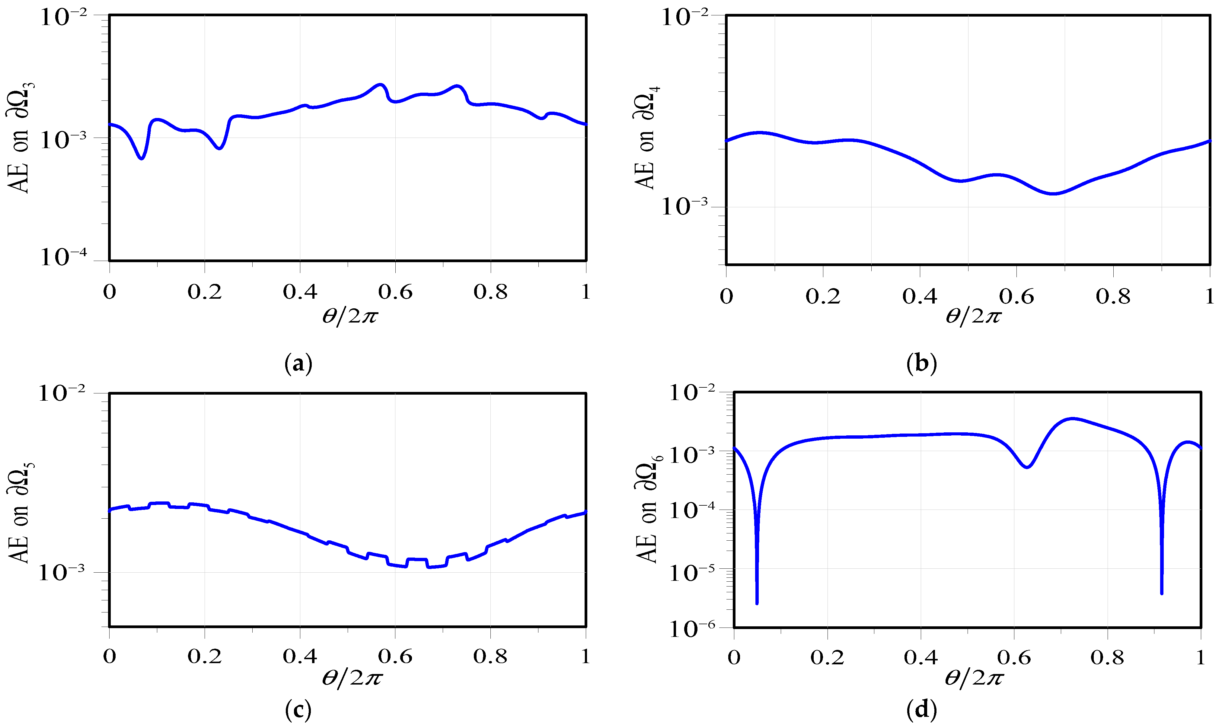
5.1. Example 1

An inverse problem of the stationary convection–diffusion equation with nine cavities enclosed by a multiply connected domain was considered. Figure 7 shows a hollow circular domain with eight circular holes with a radius of 0.125. The radii of the outer and inner circles of the hollow circular domain are 1.0 and 0.5, respectively.

The governing equation is presented in Equation (1), where $\alpha =0$, $\beta =0$, $\gamma =-900$, and $f(\mathsf{x})=(1+\gamma )(e^x+e^y)$. The boundary conditions are

$$B_{1}u(\mathsf{x})=g(\mathsf{x}),\mathsf{x}\in {\mathsf{\Omega }}_1,$$

(22)

$$B_{2}u(\mathsf{x})=h(\mathsf{x}),\mathsf{x}\in {\mathsf{\Omega }}_1.$$

(23)

The boundary data are given using the following exact solution:

$$u(\mathsf{x})=e^x+e^y.$$

(24)

Figure 8 depicts the MAE and RMSE versus the terms of the PPs. The MAE and RMSE rapidly decrease with an increase in terms, and accurate results may be obtained while the terms of the PPs are greater than 5. Figure 9 presents the error versus the dilation parameter, indicating that the value of the dilation parameter is not sensitive to the computed results and the MAE and RMSE from the proposed method are in 10⁻¹¹ and 10⁻¹³, respectively.

Additionally, we examine the influence of the location of the inner points. The layouts of the uniformly and randomly distributed inner points are depicted in Figure 10a,b, respectively. Furthermore, we consider the specified data to be polluted by random noise when the noise level is $\delta =0.03$. Figure 11 depicts the comparison of solutions along the hole boundary $\delta =0.03$. It was found that the proposed method generates results consistent with those of the analytical solution. The MAE values of the uniformly and randomly distributed inner points are in the order of ${10}^{-4}$.

Table 2. Errors of the proposed method with various wave numbers.

Wave Number	$\mathit{\omega }=50\%$		$\mathit{\omega }=25\%$
	MAE	RMSE	MAE	RMSE
100	$4.30\times {10}^{-11}$	$3.42\times {10}^{-13}$	$1.01\times {10}^{-10}$	$8.04\times {10}^{-13}$
200	$4.41\times {10}^{-11}$	$3.51\times {10}^{-13}$	$9.40\times {10}^{-11}$	$7.47\times {10}^{-13}$
300	$3.56\times {10}^{-11}$	$2.83\times {10}^{-13}$	$1.31\times {10}^{-11}$	$1.04\times {10}^{-13}$
400	$2.04\times {10}^{-11}$	$1.62\times {10}^{-13}$	$5.50\times {10}^{-11}$	$4.38\times {10}^{-13}$
500	$7.81\times {10}^{-12}$	$6.21\times {10}^{-14}$	$1.77\times {10}^{-11}$	$1.41\times {10}^{-13}$
600	$1.71\times {10}^{-11}$	$1.36\times {10}^{-13}$	$3.03\times {10}^{-10}$	$2.41\times {10}^{-12}$
700	$4.59\times {10}^{-12}$	$3.65\times {10}^{-14}$	$3.38\times {10}^{-11}$	$2.69\times {10}^{-13}$
800	$1.52\times {10}^{-11}$	$1.21\times {10}^{-13}$	$4.29\times {10}^{-11}$	$3.41\times {10}^{-13}$
900	$4.94\times {10}^{-12}$	$3.93\times {10}^{-14}$	$1.43\times {10}^{-10}$	$1.14\times {10}^{-12}$
1000	$1.25\times {10}^{-11}$	$9.93\times {10}^{-14}$	$4.70\times {10}^{-11}$	$3.74\times {10}^{-13}$

lists the errors of the proposed method with various wave numbers, and the percentages of the accessible boundary are set as $\omega =50\%$ and $\omega =25\%$. As displayed in Table 2, the MAEs utilizing the proposed method with $\omega =50\%$ and $\omega =25\%$ for $\gamma =1000$ are in the order of 10⁻¹⁴ and 10⁻¹³, respectively. The results demonstrate that the boundary data on the inaccessible boundary can be recovered even considering a large wave number.

5.2. Example 2

The governing equation is presented in Equation (1), where $\alpha =0$, $\beta =0$, $\gamma =0$, and $f\left(\mathsf{x}\right)=-\cos x-\sin y$. The boundary conditions are

$$\partial {\mathsf{\Omega }}_4=\left\{(x,y)|x=0.40+{\rho }_4(\theta )\cos \left(\theta +\frac{1}{2}\sin (8\theta )\right),y={\rho }_4(\theta )\sin \left(\theta +\frac{1}{2}\sin (8\theta )\right)\right\},$$

(25)

$$B_{1}u(\mathsf{x})=g(\mathsf{x}),\mathsf{x}\in \partial {\mathsf{\Omega }}_1,$$

(26)

$$B_{2}u(\mathsf{x})=h(\mathsf{x}),\mathsf{x}\in \partial {\mathsf{\Omega }}_1.$$

(27)

Figure 12 depicts the domain for the analysis. The boundaries are defined as follows:

$$\partial {\mathsf{\Omega }}_1=\left\{(x,y)|x={\rho }_1(\theta )\cos (\theta ),y={\rho }_1(\theta )\sin (\theta ),0\le \theta \le 2\pi \omega \right\},\omega =50\%\mathrm{and}75\%,$$

(28)

$$\partial {\mathsf{\Omega }}_2=\left\{(x,y)|x=-0.40+{\rho }_2\left(\theta \right)\cos (\theta ),y={\rho }_2\left(\theta \right)\sin (\theta )\right\},$$

(29)

$$\partial {\mathsf{\Omega }}_3=\left\{(x,y)|x={\rho }_3\left(\theta \right)\cos (\theta ),y={\rho }_3\left(\theta \right)\sin (\theta )\right\},$$

(30)

$$\partial {\mathsf{\Omega }}_4=\left\{(x,y)|x=0.40+{\rho }_4(\theta )\cos \left(\theta +\frac{1}{2}\sin (8\theta )\right),y={\rho }_4(\theta )\sin \left(\theta +\frac{1}{2}\sin (8\theta )\right)\right\},$$

(31)

in which

$${\rho }_1(\theta )=\sqrt[1/3]{\cos \left(4\theta \right)+\sqrt{\frac{18}{5}-{\sin }^2\left(4\theta \right)}},$$

(32)

$${\rho }_2(\theta )=\mathrm{abs}\left[\right(\sec 3\theta {\left)\right]}^{\sin 6\theta },$$

(33)

$${\rho }_3(\theta )=\left(3+\cos \left(\theta -\frac{\pi }{7}\right)\right)\sin \left(4\theta \right)/5+\sin \left(2\theta \right),$$

(34)

$${\rho }_4(\theta )=\sqrt[1/3]{\cos \left(3\theta \right)+\sqrt{2-{\sin }^2\left(3\theta \right)}}.$$

(35)

The analytical solution is described as

$$u(x)=\cos x+\sin y+4.$$

(36)

Two scenarios with different accessible boundaries are investigated. The locations of the collocation points for cases A and B are depicted in Figure 12a,b, respectively. The error of the proposed method with different terms of the PPs is investigated, as shown in Figure 13a. Highly accurate results are obtained while the terms are greater than 4. The RMSE is in the order of 10⁻¹⁰ if the terms of the PPs range between 5 and 20. Consequently, the terms of the PPs are set as 11 in this example. Figure 13b illustrates the error versus the dilation parameter for case B. Accurate results are obtained for the dilation parameter from 2 to 5.

The MAE and RMSE versus different noise levels for cases A and B are represented in Figure 14a,b, respectively. The RMSE values associated with the proposed approach for cases A and B are in the order of 10⁻⁵ and 10⁻⁵, respectively. Figure 15 displays the computed results with different noise levels. Results obtained indicate that our approach obtains highly accurate results, as shown in Figure 16.

5.3. Example 3

The governing equation is presented in Equation (1), where $\alpha =y^3\sin x$, $\beta =-y^2\cos x$, $\gamma =x^{2}y$ and $f\left(\mathsf{x}\right)=y\cos (x)+x\cos (y)$. The following analytical solution is adopted for validation

$$u(x,y)=y\cos (x)+x\cos (y).$$

(37)

The boundary data are expressed as

$$B_{1}u(\mathsf{x})=g(\mathsf{x}),\mathsf{x}\in \partial {\mathsf{\Omega }}_1,\mathrm{and}$$

(38)

$$B_{2}u(\mathsf{x})=h(\mathsf{x}),\mathsf{x}\in \partial {\mathsf{\Omega }}_1.$$

(39)

Figure 17 depicts a multiply connected domain for this example. The boundaries are defined as follows:

$$\begin{gathered} \partial {\mathsf{\Omega }}_1=\left\{(x,y)|x={\rho }_1\left(\theta \right)\cos \left(\theta \right),y={\rho }_1\left(\theta \right)\sin \left(\theta \right),0\le \theta \le 2\pi \omega \right\}, \\ \omega =75\%\mathrm{and}50\%, \end{gathered}$$

(40)

$$\partial {\mathsf{\Omega }}_2=\left\{(x,y)|x=-0.22+{\rho }_2\left(\theta \right)\cos \left(\theta \right),y={\rho }_2\left(\theta \right)\sin \left(\theta \right)\right\},$$

(41)

$$\partial {\mathsf{\Omega }}_3=\left\{(x,y)|x={\rho }_3\left(\theta \right)\cos \left(\theta \right),y=0.25+{\rho }_3\left(\theta \right)\sin \left(\theta \right)\right\},$$

(42)

$$\partial {\mathsf{\Omega }}_4=\left\{(x,y)|x=0.25+{\rho }_4\left(\theta \right)\cos \left(\theta \right),y={\rho }_4\left(\theta \right)\sin \left(\theta \right)\right\},\mathrm{and}$$

(43)

$$\partial {\mathsf{\Omega }}_5=\left\{(x,y)|x={\rho }_5\left(\theta \right)\cos \left(\theta \right),y=-0.25+{\rho }_5\left(\theta \right)\sin \left(\theta \right)\right\},$$

(44)

in which

$${\rho }_1(\theta )=\sqrt[1/3]{\cos \left(4\theta \right)+\sqrt{\frac{18}{5}-{\sin }^2\left(4\theta \right)}},$$

(45)

$${\rho }_2(\theta )=\mathrm{abs}{(\sec (3\theta ))}^{\sin (6\theta )},$$

(46)

$${\rho }_3(\theta )=\left(3+\cos \left(\theta -\frac{\pi }{7}\right)\right)\sin \left(4\theta \right)/5+\sin \left(2\theta \right),$$

(47)

$${\rho }_4(\theta )=1+\frac{1}{10}\tan \mathrm{h}\left(10\sin \left(2\theta \right)\right),\mathrm{and}$$

(48)

$${\rho }_5(\theta )=\sqrt[1/3]{\cos \left(3\theta \right)+\sqrt{2-{\sin }^2\left(3\theta \right)}}.$$

(49)

In this example, the dilation parameter and the PPs terms are 2 and 11, respectively. Two scenarios with different accessible boundaries are investigated. The configurations of the collocation points for cases C and D are illustrated in Figure 17. The percentages of the accessible boundary for cases C and D are 75% and 50%, respectively.

The error of the proposed approach with different terms of the PPs is investigated, as shown in Figure 18a. Highly accurate results are acquired while the terms are greater than 4. The RMSE is in the order of 10⁻⁹, with the terms ranging from 5 to 20. Figure 18b illustrates the error versus the terms for case D. Accurate results may be achieved while the dilation parameter is from 2 to 5. Furthermore, the dilation parameter may be less sensitive to accuracy.

The MAE and RMSE versus different noise levels for cases C and D are shown in

Table 3. Errors of the proposed method with various noise levels.

Noise Level	Case C		Case D
	MAE	RMSE	MAE	RMSE
${10}^{-6}$	$1.03\times {10}^{-7}$	$2.79\times {10}^{-10}$	$1.37\times {10}^{-6}$	$3.68\times {10}^{-9}$
${10}^{-5}$	$1.07\times {10}^{-6}$	$4.83\times {10}^{-9}$	$1.58\times {10}^{-5}$	$2.91\times {10}^{-8}$
${10}^{-4}$	$1.94\times {10}^{-6}$	$1.98\times {10}^{-8}$	$1.88\times {10}^{-5}$	$3.53\times {10}^{-8}$
${10}^{-3}$	$6.59\times {10}^{-5}$	$2.52\times {10}^{-7}$	$1.14\times {10}^{-4}$	$6.45\times {10}^{-7}$
$0.01$	$2.80\times {10}^{-3}$	$6.00\times {10}^{-6}$	$2.10\times {10}^{-3}$	$7.27\times {10}^{-6}$
$0.02$	$1.20\times {10}^{-3}$	$4.08\times {10}^{-6}$	$3.50\times {10}^{-3}$	$1.28\times {10}^{-5}$
$0.03$	$1.30\times {10}^{-3}$	$6.51\times {10}^{-6}$	$5.20\times {10}^{-3}$	$1.62\times {10}^{-5}$

. Figure 19 displays the computed results with the different noise levels. Our method yields highly accurate results shown in Figure 20. The MAE of our method can reach 10⁻³ with $\delta =0.03$, as depicted in Figure 21.

6. Discussion

A linear combination of polyharmonic RBFs plus a polynomial term is the common way to construct the polyharmonic spline. The polyharmonic splines are often used for function approximation, which is provided for interpolating and fitting scattered data in different dimensions. The polyharmonic splines are the combination of many polyharmonic RBFs at different centers in which a certain order of each polyharmonic RBF is fixed. The polynomial term may improve fitting accuracy for the polyharmonic spline. However, the polynomial term is separated from the polyharmonic RBF, which needs to be defined by the users. Additionally, the certain order of the polyharmonic RBF depends on the types of problems to be solved; it is often challenging to determine the certain order of the polyharmonic RBF.

In this study, we proposed a pioneering work to apply the RBF method with polyharmonic polynomials in which the polynomial term is not required prior. The polyharmonic polynomials are a series of polyharmonic RBFs that have many radial polynomials. Since the polyharmonic polynomials include only the radial terms, the proposed polyharmonic polynomials have the advantages of a simple mathematical expression, high precision, and easy implementation.

We also conducted the parametric analysis in the sections of validation and numerical examples. It was found that the MAE and RMSE versus the order of the proposed polyharmonic polynomials exhibited that accurate solutions can be obtained while the terms of the polyharmonic polynomials are greater than 5. Additionally, accurate solutions can be obtained with the terms of the polyharmonic polynomials no greater than 10 for all numerical examples. Finally, we may conclude that the proposed polyharmonic polynomials may resolve the challenge of determining the certain order of the polyharmonic RBF in the conventional polyharmonic spline. Additionally, an accurate solution can be obtained with the increase in terms for polyharmonic polynomials.

7. Conclusions

In this study, a pioneering work applies the RBF method with polyharmonic polynomials to model the movement of contaminants based on the stationary convection–diffusion equation. The concept of the proposed approach is addressed in detail. Significant findings are concluded as follows.

(1)

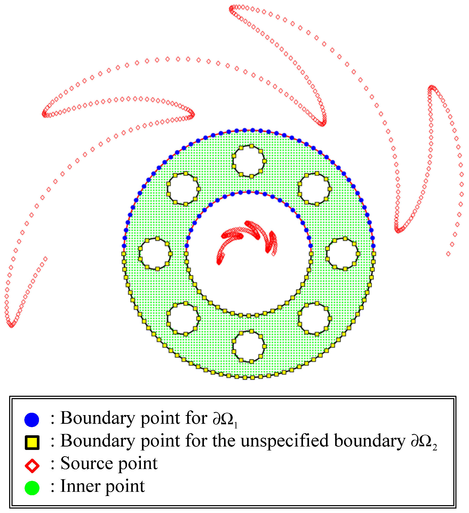
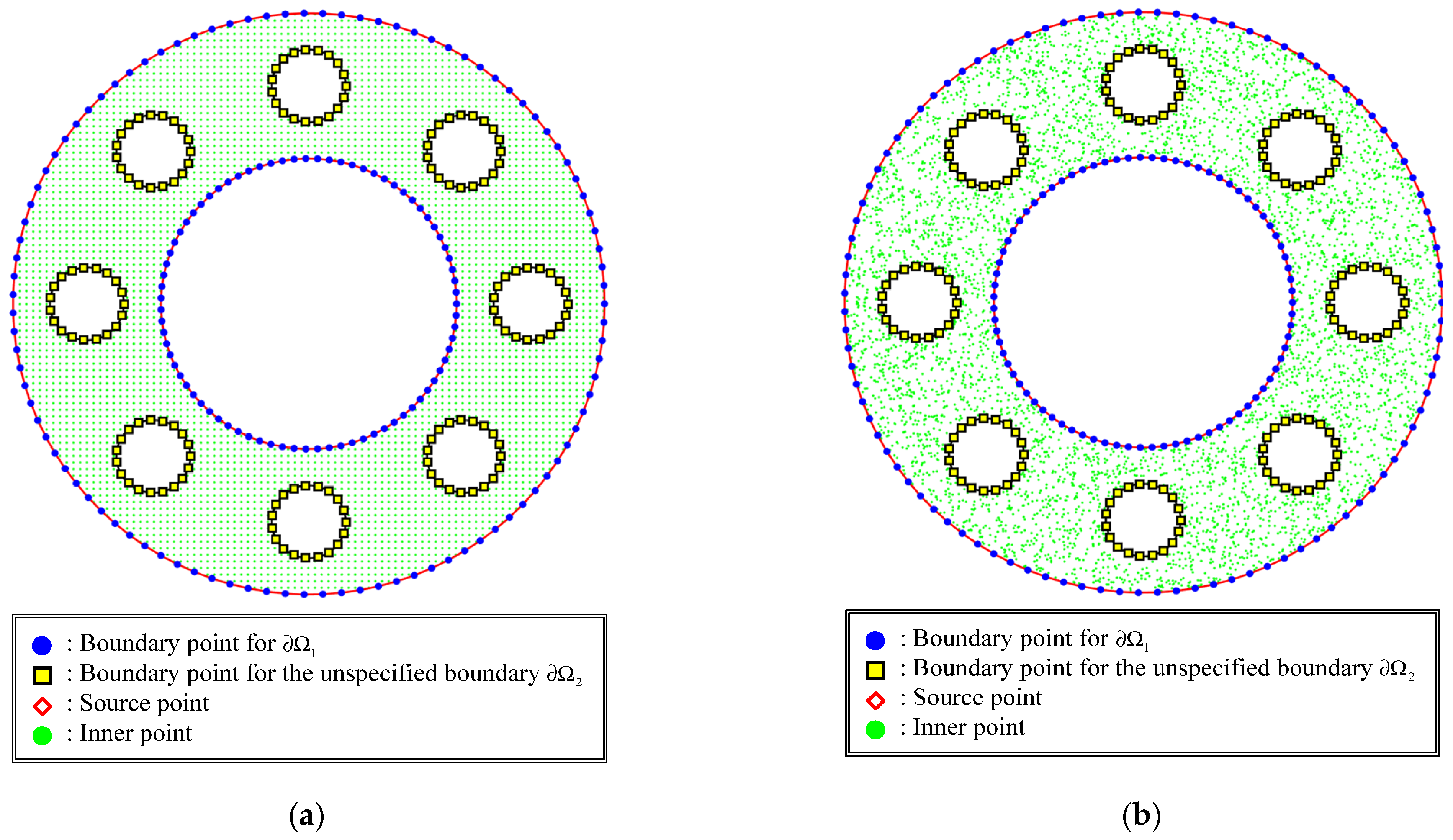
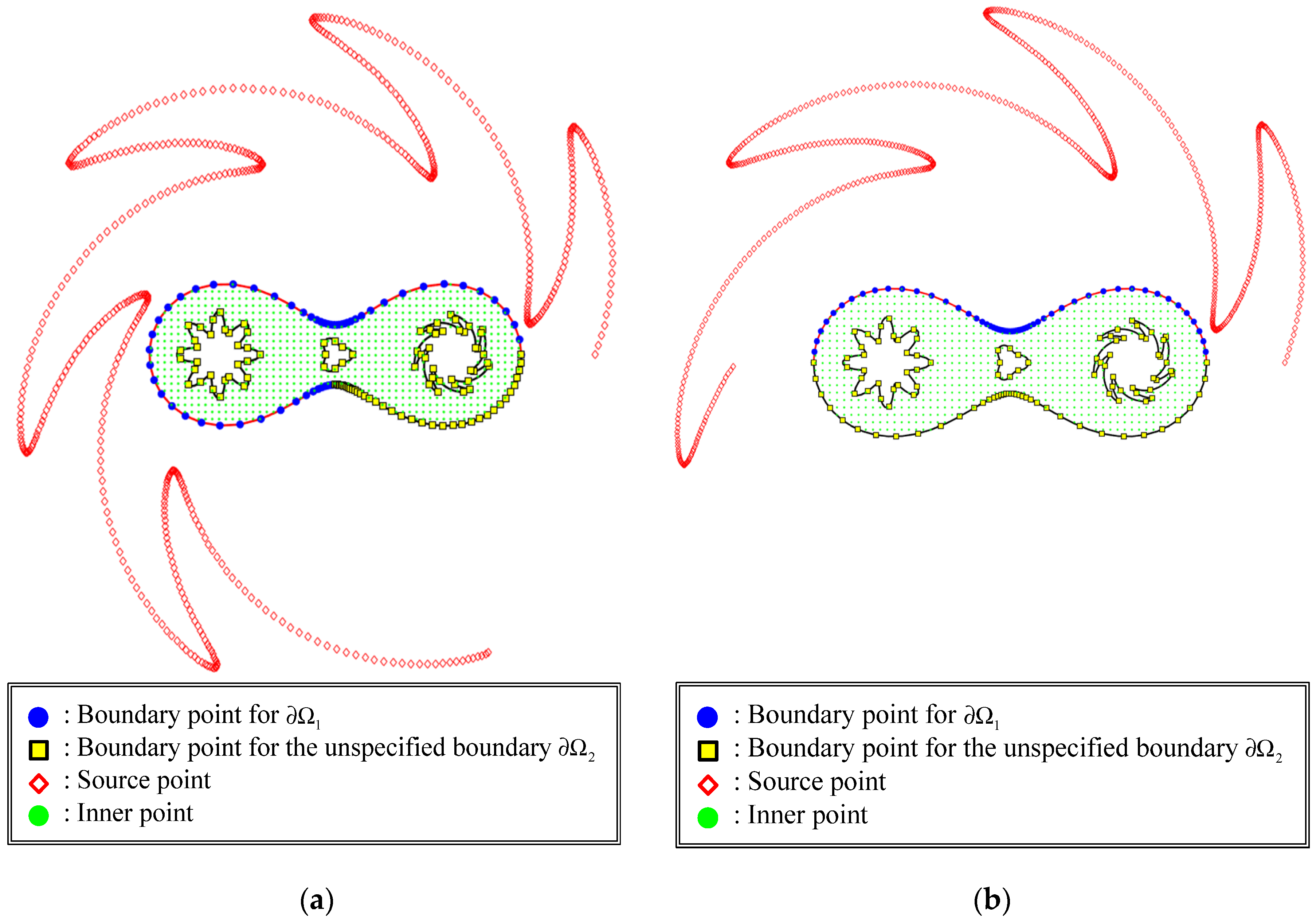
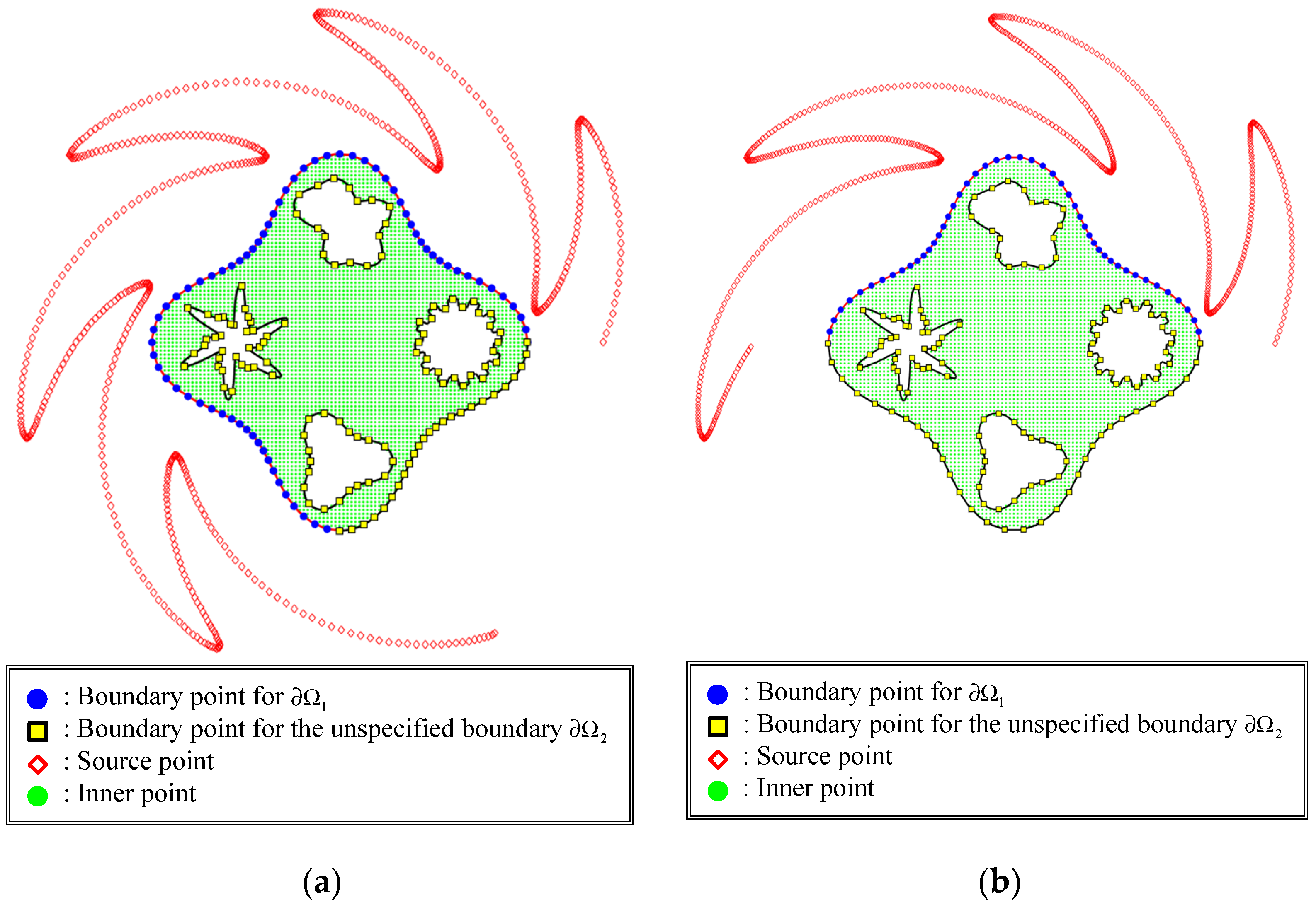
In this study, we demonstrated that the radial basis function method with polyharmonic polynomials could achieve accurate results for inverse problems of the stationary convection–diffusion equation. Due to the meshless nature, the proposed RBF method is superior to solving the inverse problems in groundwater pollution problems with highly complicated domains such as the multiply-connected domains containing a finite number of cavities;

(2)

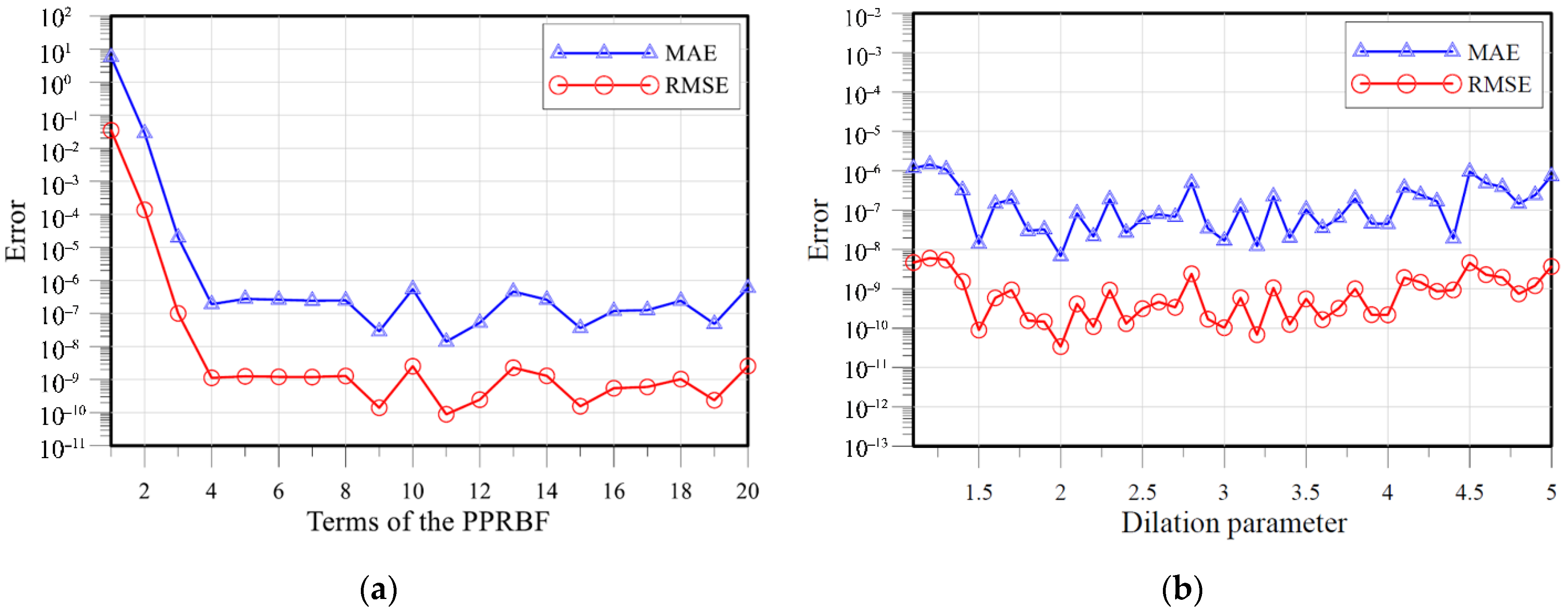
The polyharmonic RBFs with a certain order are often used for function approximation. Because the order of the conventional polyharmonic RBF is fixed and needs to be given prior to the analysis, it is often challenging to determine the certain order of the polyharmonic RBF. In this study, we proposed polyharmonic polynomials (PPs). The PPs are a series of polyharmonic RBFs, including any order of the polyharmonic RBFs. Accordingly, the order of the polyharmonic RBF is not required to be given prior to the analysis;

(3)

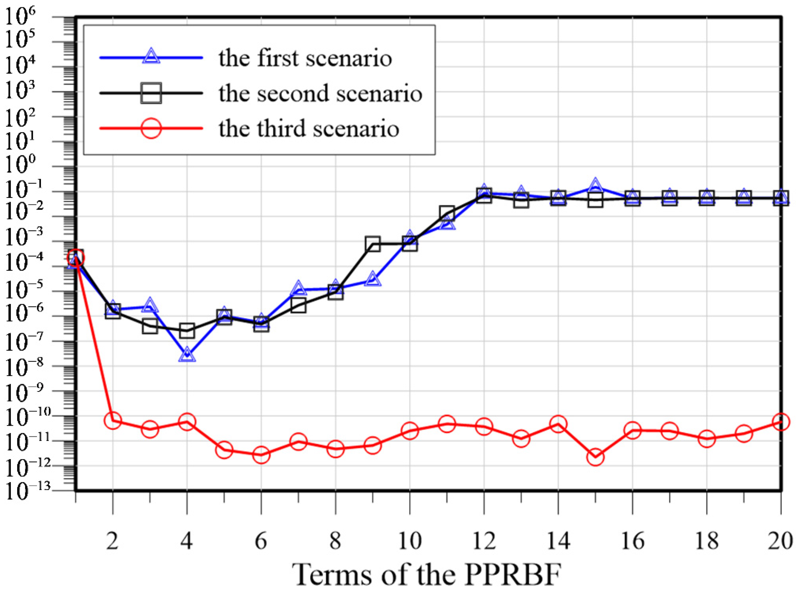
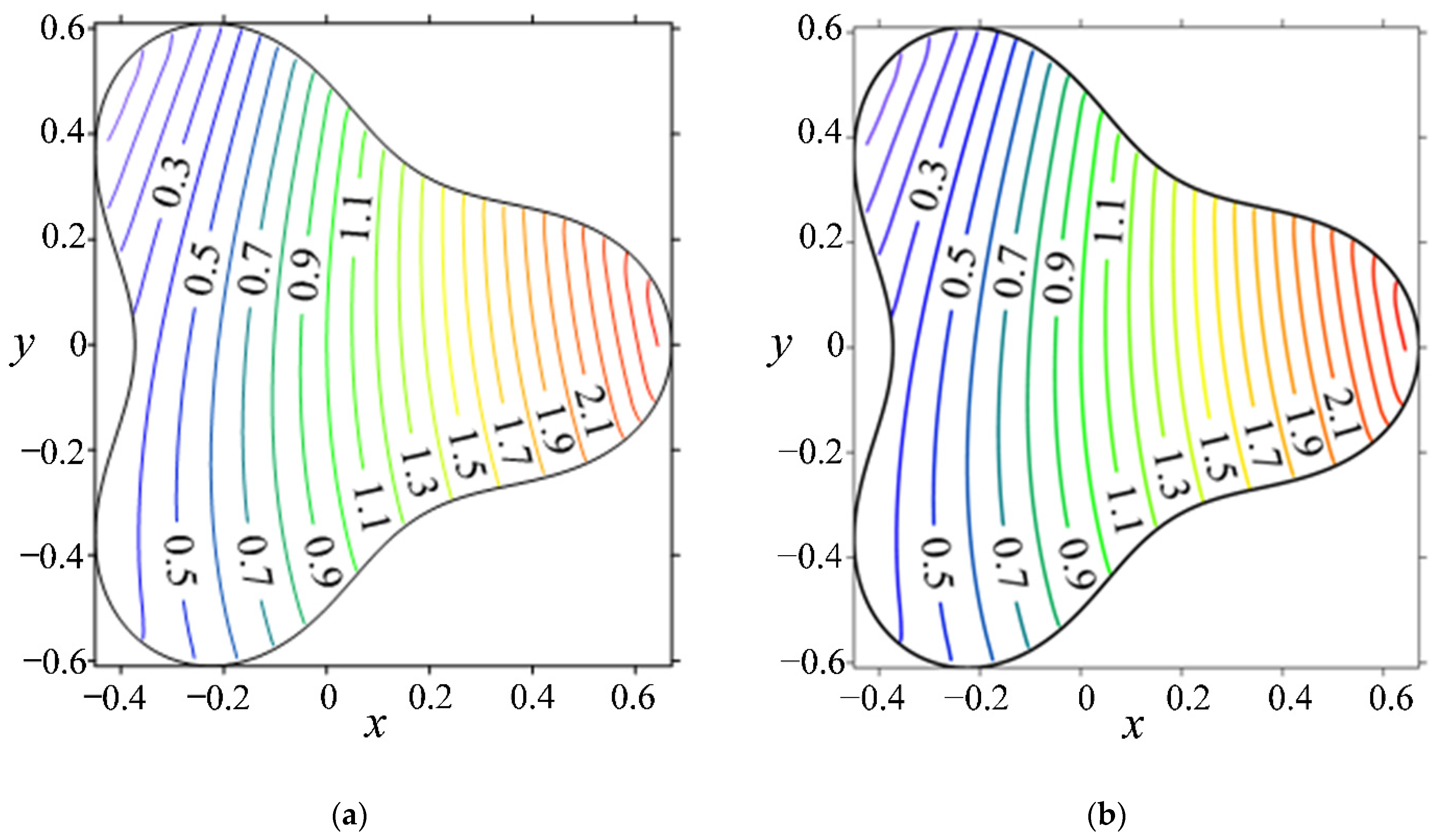
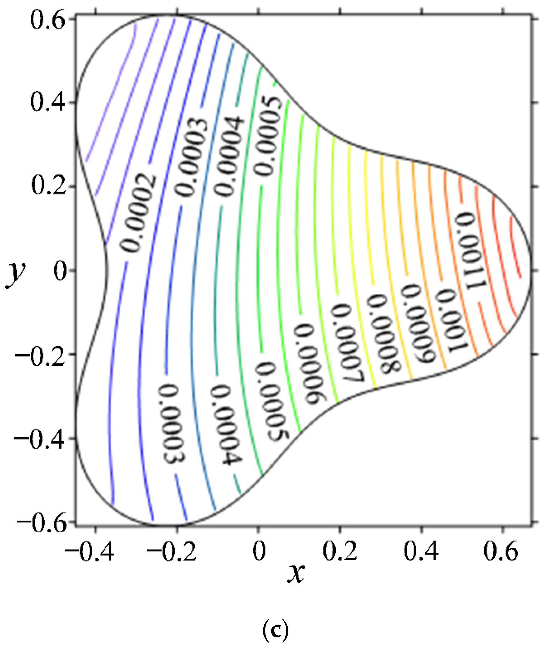
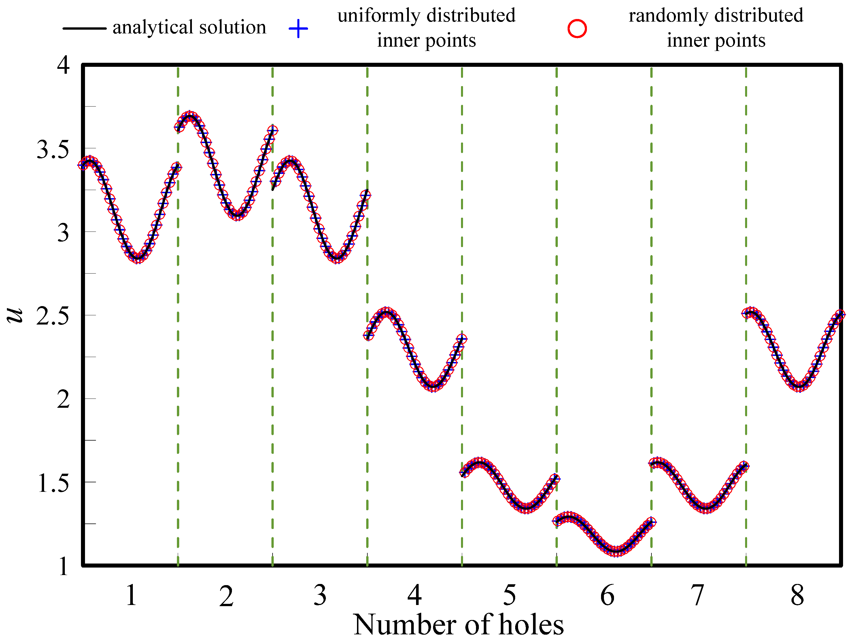
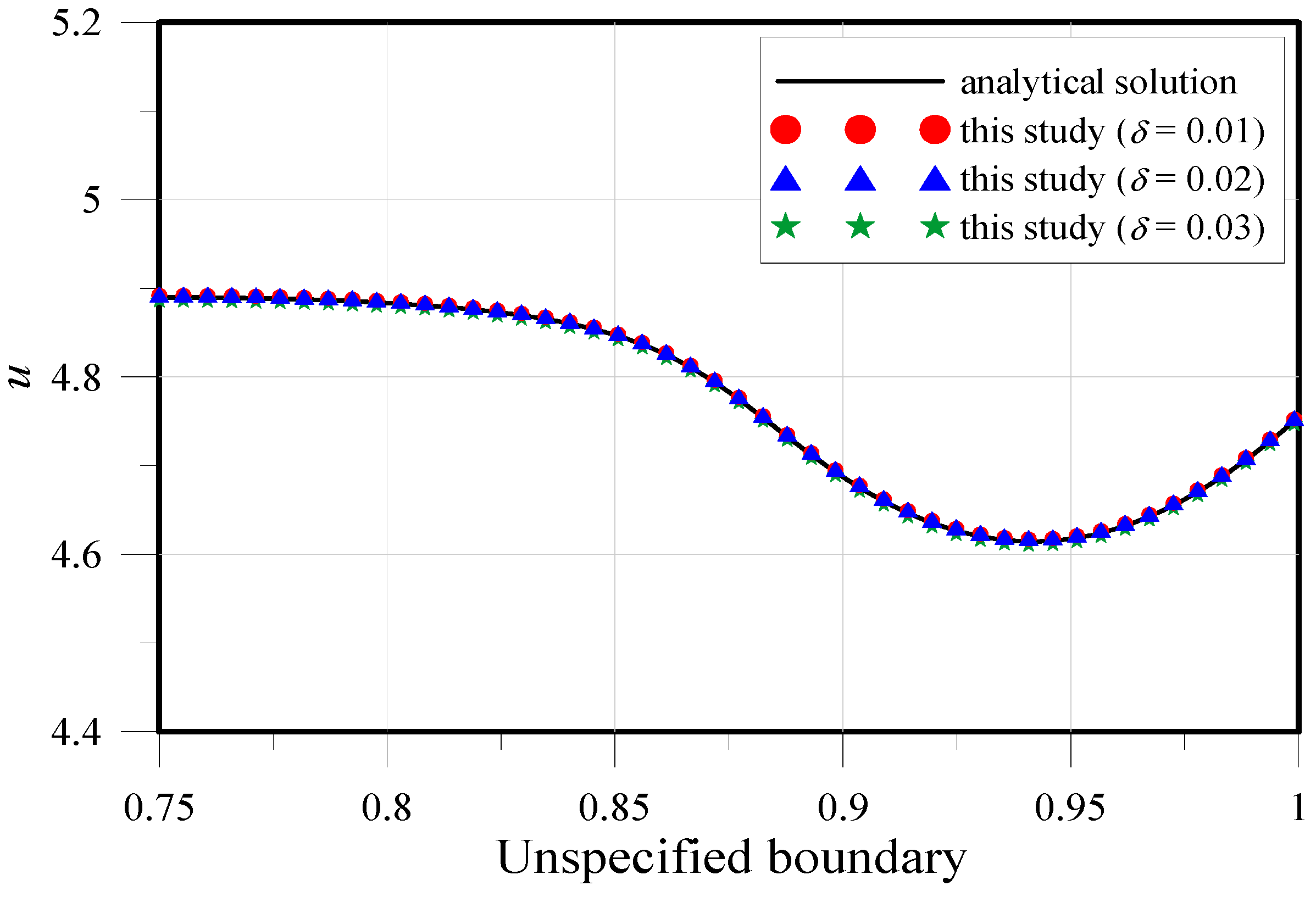
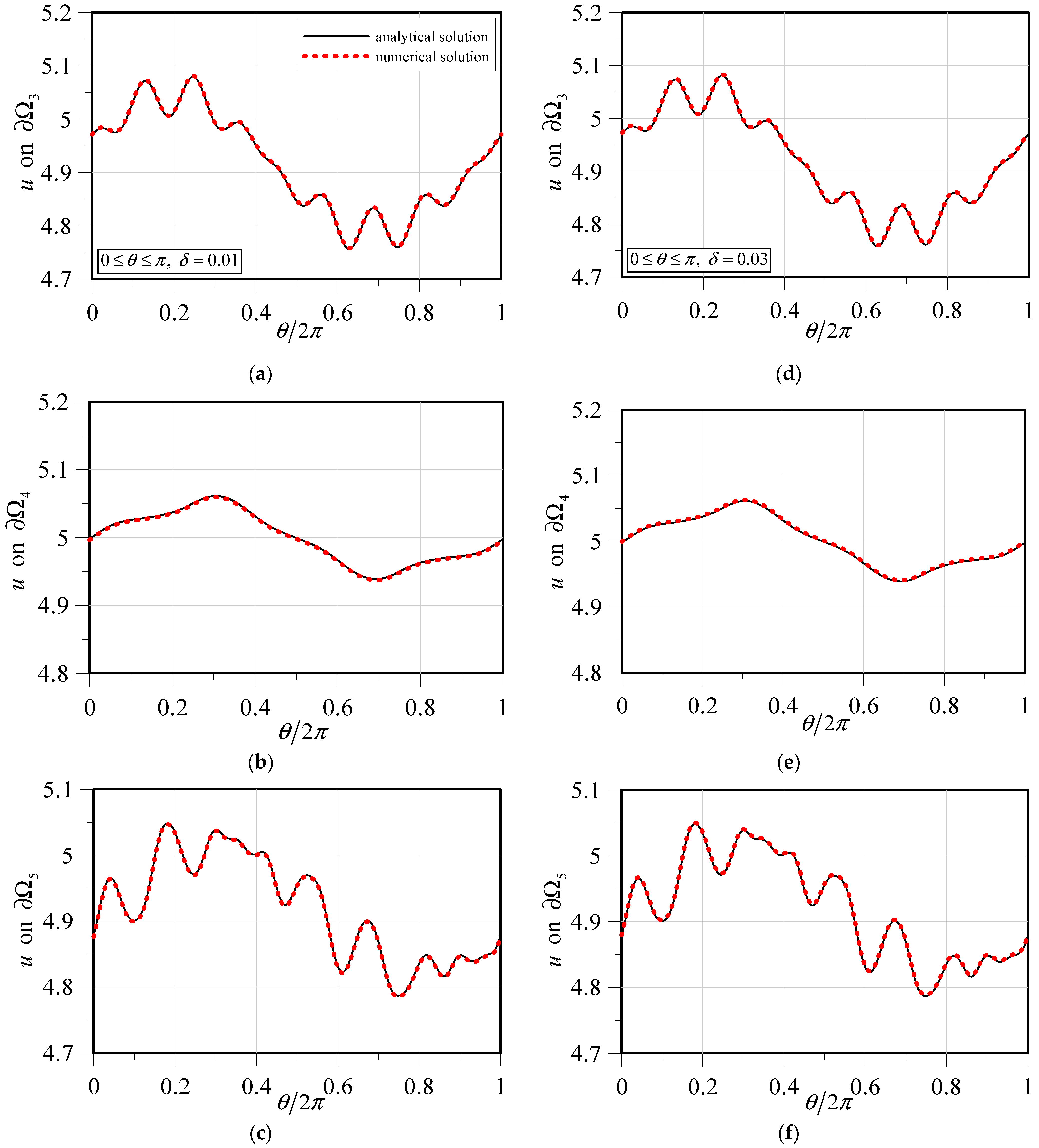
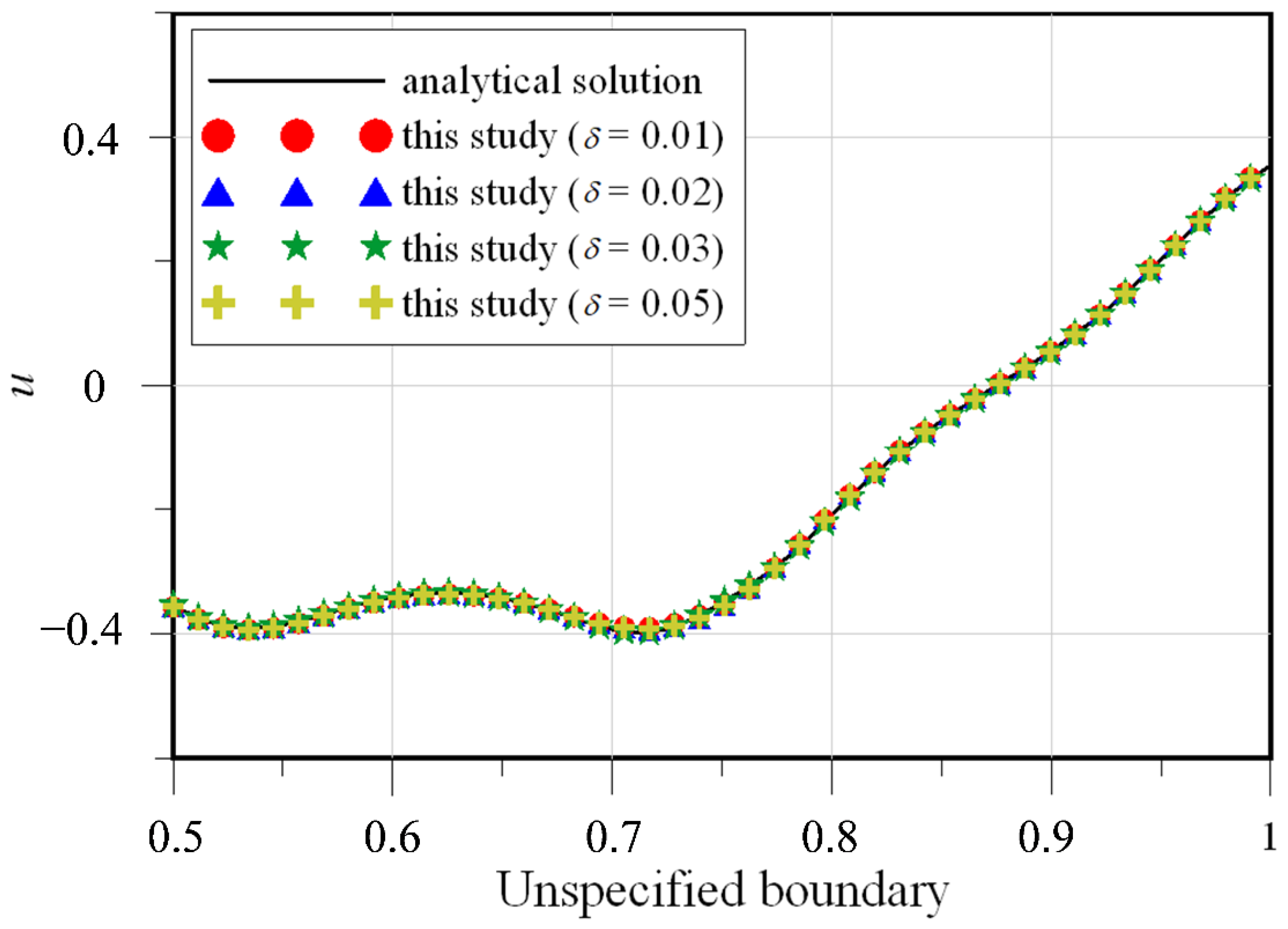
Numerical examples in simply and multiply connected domains such as cavities with complicated shapes were carried out. We may recover the missing boundary observations such as concentration on the remaining boundary or those of the cavities with highly accurate results using more terms of the PPs;

(4)

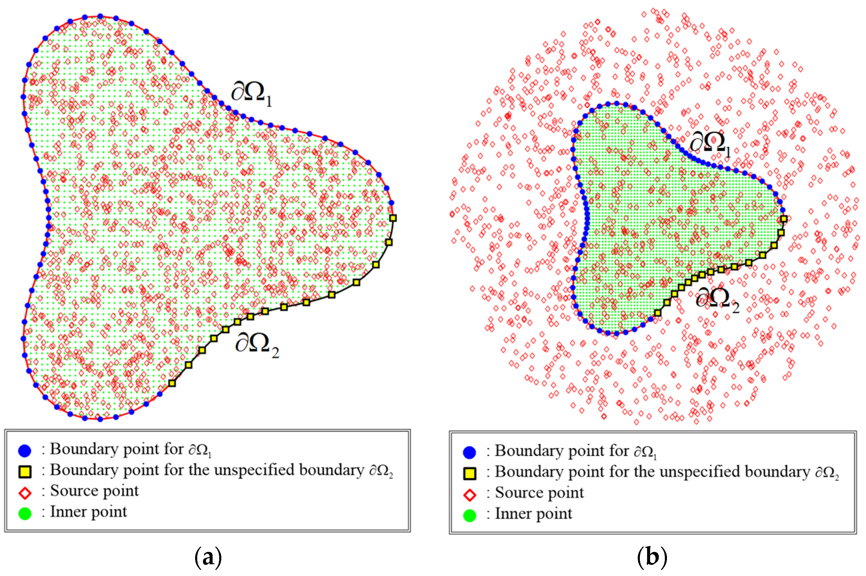
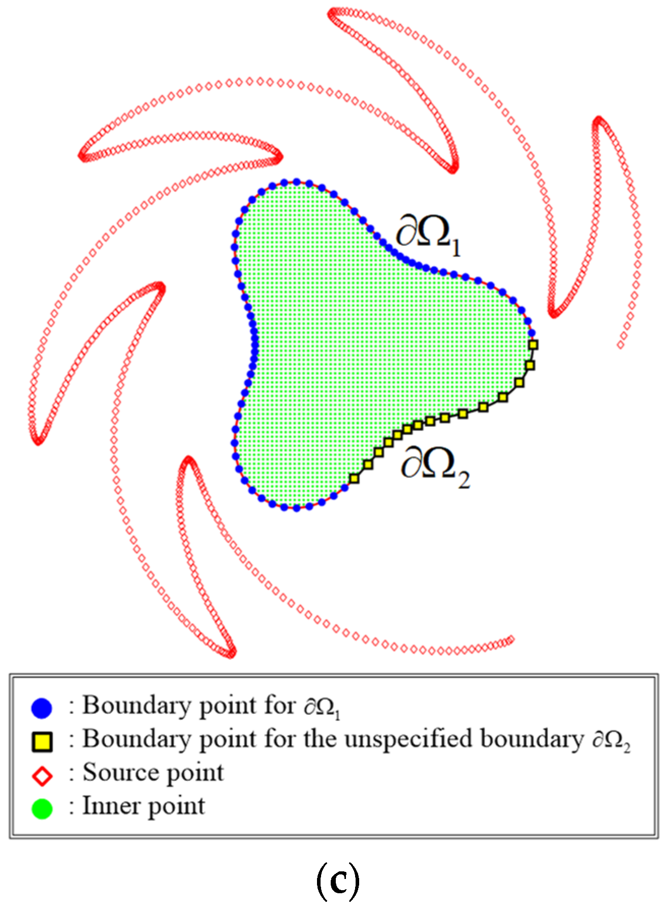
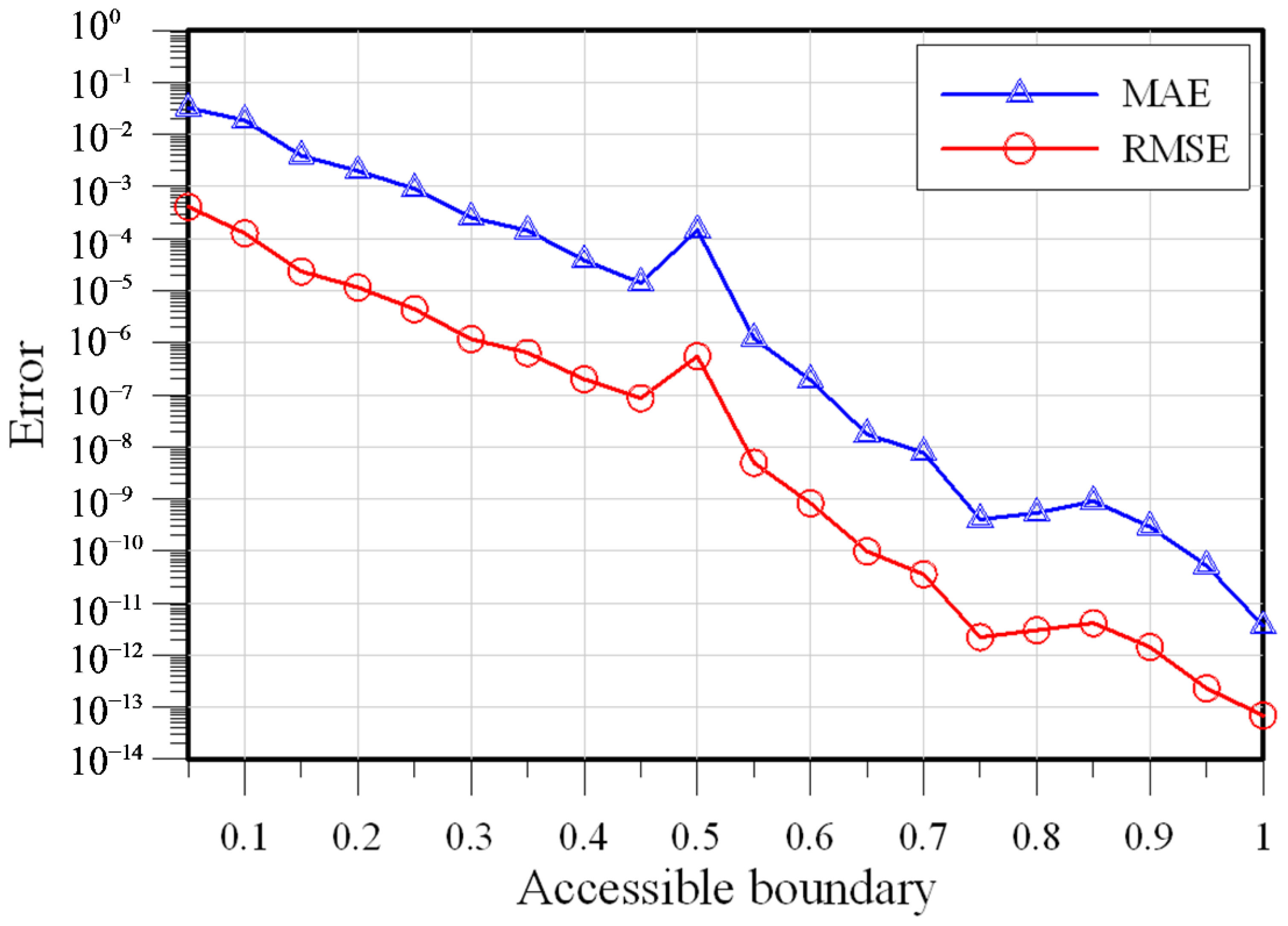
Comparative analysis was conducted for three different scenarios for collocating sources, such as sources inside the domain randomly, random sources within a circle containing the domain, and sources outside the domain. It was found that the sources collocated outside the domain exhibit the best accuracy;

(5)

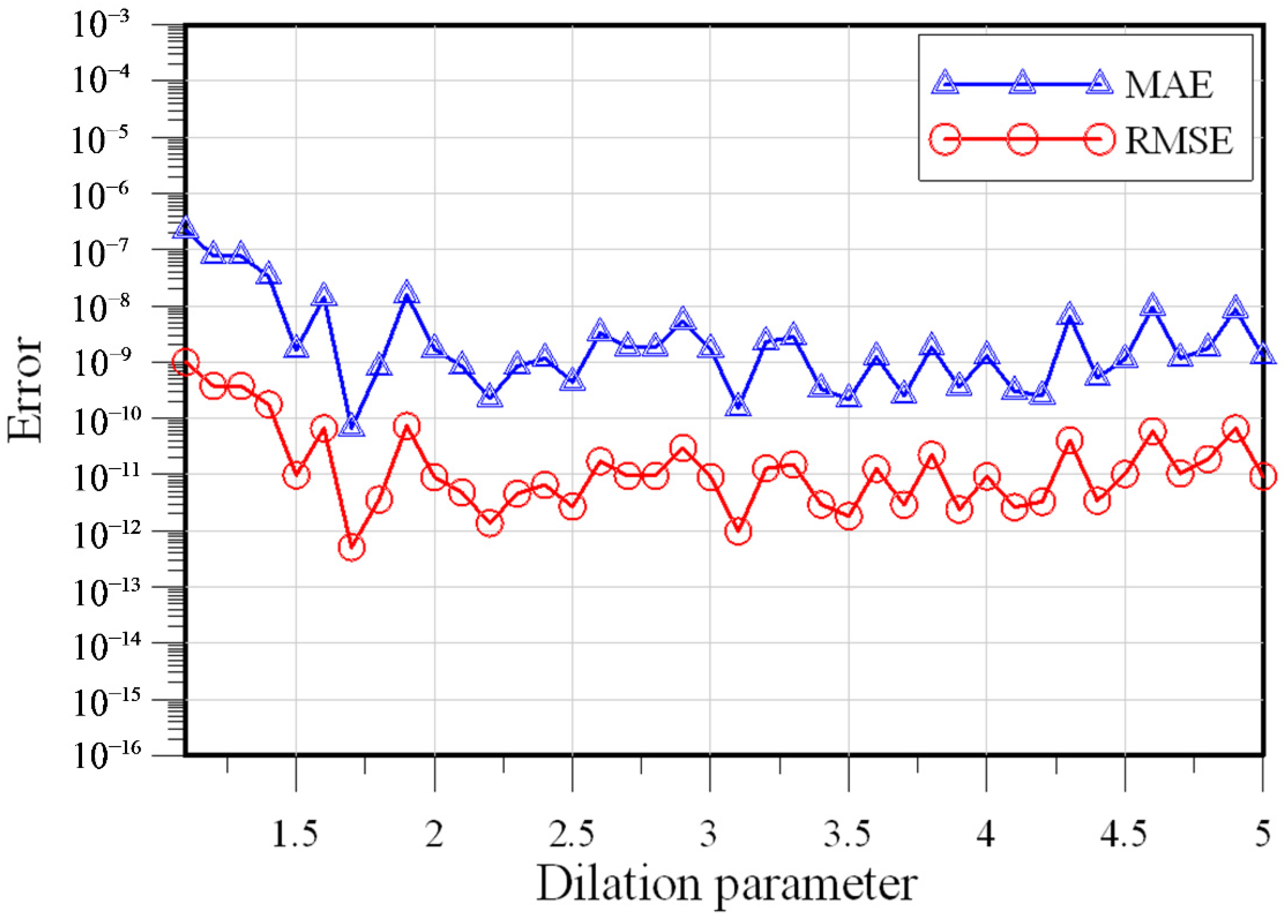
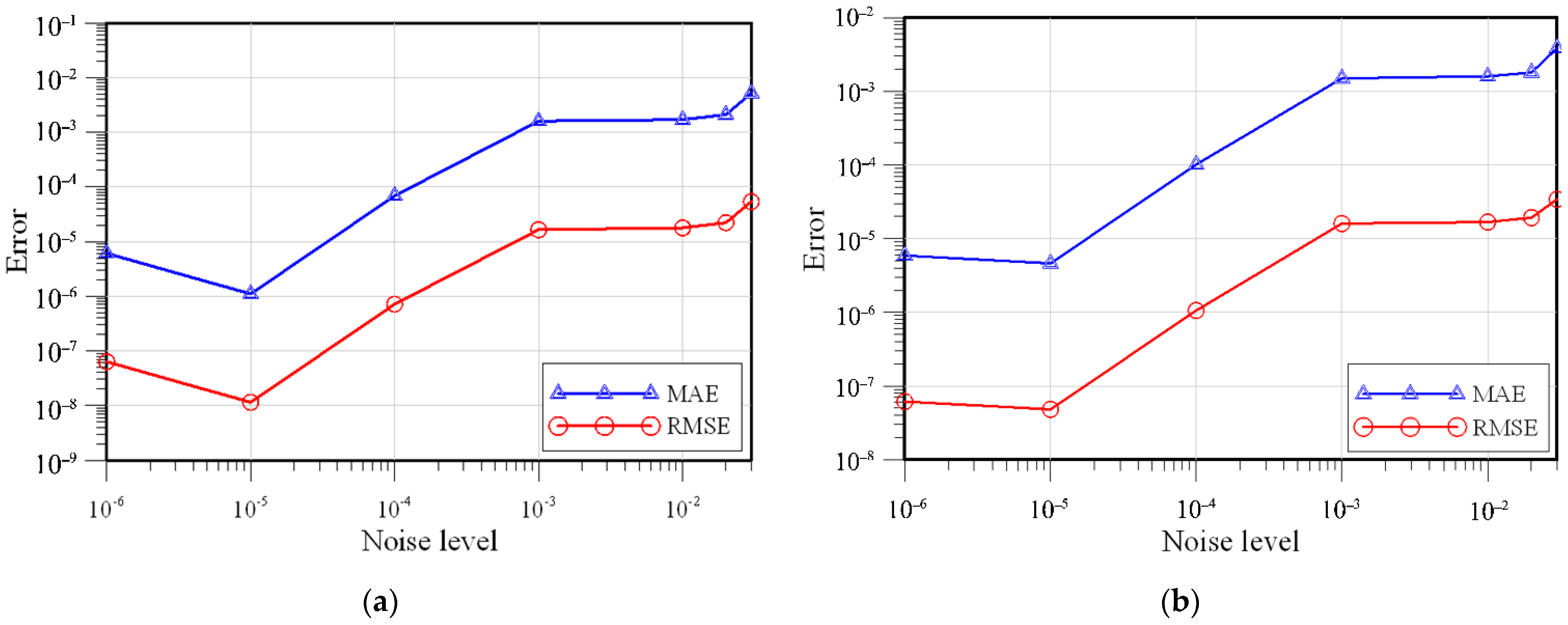
The results depict that the proposed method could recover highly accurate solutions for inverse problems of the stationary convection–diffusion equation with cavities even with 5% noisy data. Moreover, the proposed method is a meshfree method and collocation only such that we can solve the inverse problems with highly complicated domain shapes easily and efficiently;

(6)

In this study, a pioneering work attempted to apply the radial basis function method with PPs for inverse problems with very complicated domains. We achieved a promising result for multiply connected domains containing a finite number of cavities. Further studies to investigate the characteristics of the proposed method to solve inverse problems in three dimensions are suggested.

References

- Oruç, Ö. A meshless multiple-scale polynomial method for numerical solution of 3d convection–diffusion problems with variable coefficients. Eng. Comput. 2020, 36, 1215–1228. [Google Scholar] [CrossRef]
- Chang, C.-M.; Ma, K.-C.; Chuang, M.-H. Temporal variability in the response of a linear time-invariant catchment system to a non-stationary inflow concentration field. Appl. Sci. 2020, 10, 5356. [Google Scholar] [CrossRef]
- Srivastava, M.H.; Ahmad, H.; Ahmad, I.; Thounthong, P.; Khan, N.M. Numerical simulation of three-dimensional fractional-order convection-diffusion PDEs by a local meshless method. Therm. Sci. 2020, 210, 1–14. [Google Scholar]
- Rap, A.; Elliott, L.; Ingham, D.B.; Lesnic, D.; Wen, X. The inverse source problem for the variable coefficients convection-diffusion equation. Inverse Probl. Sci. Eng. 2007, 15, 413–440. [Google Scholar] [CrossRef]
- Liu, J.; Zhang, J.; Zhang, X. Semi-discretized numerical solution for time fractional convection–diffusion equation by RBF-FD. Appl. Math. Lett. 2022, 128, 107880. [Google Scholar] [CrossRef]
- Boyce, S.E.; Yeh, W.W.G. Parameter-independent model reduction of transient groundwater flow models: Application to inverse problems. Adv. Water Resour. 2014, 69, 168–180. [Google Scholar] [CrossRef]
- Pyatkov, S.G. Some classes of inverse problems of determining the source function in convection–diffusion systems. Differ. Equ. 2017, 53, 1352–1363. [Google Scholar] [CrossRef]
- Ku, C.Y.; Hong, L.D.; Liu, C.Y. Solving transient groundwater inverse problems using space–time collocation Trefftz method. Water 2020, 12, 3580. [Google Scholar] [CrossRef]
- Gurarslan, G.; Karahan, H. Solving inverse problems of groundwater-pollution-source identification using a differential evolution algorithm. Hydrogeol. J. 2015, 23, 1109–1119. [Google Scholar] [CrossRef]
- Golmohammadi, A.; Khaninezhad, M.R.M.; Jafarpour, B. Group-sparsity regularization for ill-posed subsurface flow inverse problems. Water Resour. Res. 2015, 51, 8607–8626. [Google Scholar] [CrossRef]
- Liu, C.S.; Wang, F. A meshless method for solving the nonlinear inverse Cauchy problem of elliptic type equation in a doubly-connected domain. Comput. Math. Appl. 2018, 76, 1837–1852. [Google Scholar] [CrossRef]
- Sarra, S.A. A local radial basis function method for advection–diffusion–reaction equations on complexly shaped domains. Appl. Math. Comput. 2012, 218, 9853–9865. [Google Scholar] [CrossRef] [Green Version]
- Uddin, M. RBF-PS scheme for solving the equal width equation. Appl. Math. Comput. 2013, 222, 619–631. [Google Scholar] [CrossRef]
- Liu, C.S.; Wang, P. An analytic adjoint Trefftz method for solving the singular parabolic convection–diffusion equation and initial pollution profile problem. Int. J. Heat Mass Transf. 2016, 101, 1177–1184. [Google Scholar] [CrossRef]
- Shivanian, E. Local radial basis function interpolation method to simulate 2D fractional-time convection-diffusion-reaction equations with error analysis. Numer. Meth. Part Differ. Equ. 2017, 33, 974–994. [Google Scholar] [CrossRef]
- Liu, C.Y.; Ku, C.Y.; Xiao, J.E.; Yeih, W. A novel spacetime collocation meshless method for solving two-dimensional backward heat conduction problems. Comp. Model. Eng. Sci. 2019, 118, 229–252. [Google Scholar] [CrossRef] [Green Version]
- Valencia, C.; Yuan, M. Radial basis function regularization for linear inverse problems with random noise. J. Multivar. Anal. 2013, 116, 92–108. [Google Scholar] [CrossRef]
- Khan, M.N.; Ahmad, I.; Ahmad, H. A radial basis function collocation method for space-dependent inverse heat problems. J. Appl. Comput. Mech. 2015, 8, 239–254. [Google Scholar]
- Golbabai, A.; Kalarestaghi, N. Improved localized radial basis functions with fitting factor for dominated convection-diffusion differential equations. Eng. Anal. Bound. Elem. 2018, 92, 124–135. [Google Scholar] [CrossRef]
- Rashidinia, J.; Khasi, M.; Fasshauer, G.E. A stable Gaussian radial basis function method for solving nonlinear unsteady convection–diffusion–reaction equations. Comput. Math. Appl. 2018, 75, 1831–1850. [Google Scholar] [CrossRef]
- Liu, C.Y.; Ku, C.Y.; Hong, L.D.; Hsu, S.M. Infinitely smooth polyharmonic RBF collocation method for numerical solution of elliptic PDEs. Mathematics 2021, 9, 1535. [Google Scholar] [CrossRef]
- Santos, L.G.C.; Manzanares-Filho, N.; Menon, G.J.; Abreu, E. Comparing RBF-FD approximations based on stabilized Gaussians and on polyharmonic splines with polynomials. Int. J. Numer. Methods Eng. 2018, 115, 462–500. [Google Scholar] [CrossRef]
- Ku, C.Y.; Liu, C.Y.; Xiao, J.E.; Hsu, S.-M.; Yeih, W. A collocation method with space–time radial polynomials for inverse heat conduction problems. Eng. Anal. Bound. Elem. 2021, 122, 117–131. [Google Scholar] [CrossRef]