1. Introduction
Agriculture in the world plays an important role in feeding the population. Agriculture has recently been threatened by the availability of water and has generated concern about the use of water in the world, leaving much to be desired in agriculture as it has generated an unsustainable situation [
1] For this reason, smart irrigation systems were created to optimize water use in crops and improve productivity [
2].
The development of the 21st century is still largely based on agriculture with activities in agribusiness, taking into consideration climate change, soil and irrigation factors in almost all regions, for this, a study [
3] was conducted using artificial neural networks (ANN) that analyzes the smart agriculture dataset with parameters such as temperature, soil moisture, wind speed, solar radiation and soil water tension.
Agriculture has played an important role in the development of every country, therefore, automation has been increased the area of irrigation with smart technology in some cases through embedded systems that concentrates on controlling the irrigation process automatically using a Raspberry Pi device through Python programming with the help of moisture sensors that monitor the soil [
4]. The level of irrigation depends on the soil moisture content and crop type, which reduces the overall energy consumption and optimizes the use of water reserves, a low-cost Arduino-based smart irrigation solution [
5].
The advancement in automation techniques allows improving crop yields, making them more profitable and reducing irrigation wastage by having sensors deployed in an agricultural field, which sends data through a microprocessor via Internet of Things (IoT) devices with the cloud, through a decision tree algorithm, which sends an alert by mail to farmers and allows the decisions on water supply to be made in advance [
6]. Automation through irrigation scheduling has been achieved by several methods, such as the measurement of environmental variables used for control, simulation of irrigation strategies that allows forecasting conditions for crops without damaging the crops and then being applied in the field [
7].
Automated irrigation is based on parameters monitored from a meteorological station that indicates parameters such as crop water demand, soil, evapotranspiration, precipitation, climatic conditions, etc., which are used to analyze the data in various scenarios and to propose strategies and control methods where irrigation efficiency analysis can be applied [
8]. Through simulation, the performance of proposals can be validated, so [
9] shows a control algorithm with a database that forecasts crop yield and manages water resources, closed-loop control is performed and through feedback from weather conditions the model anticipates the crop water demand and to generate the irrigation scheduling of water consumption [
10].
Although water resources are available in many countries, global warming, pollution and losses due to the misapplication of water are considerable and inappropriate types of risks have been generated, affecting the efficient use of water [
11]. Agricultural irrigation is mostly done manually/mechanically without considering the amount of water needed for the crop. With the help of technology, it is possible to create smart irrigation systems that focus on saving water and energy and obtaining a higher quality in the final product [
12].
Different projects have been carried out in different sectors of smart irrigation systems with fuzzy logic based on rules, by sensing soil moisture and meteorological variables and managing the flow of water through an agronomic design [
12]. The smart irrigation design in vegetables implemented in a university is managed through a graphical interface, allowing the automation of irrigation using fuzzy logic compared to manual drip irrigation [
13]. In rural areas, irrigation control is performed by comparing environmental parameters with sensors located along the crop, electrovalves as actuators that control the water flow and thus obtain greater efficiency and less water waste [
14]. Although these studies have contributed to the improvement of irrigation, they do not consider the future state of irrigation variables, so their decisions are not the most optimal.
Optimal irrigation has not been fully addressed with smart tools, such as model-based predictive control (MPC), which allow the improvement of agricultural production at low costs by taking advantage of optimally managed natural resources and analyzing the technical feasibility of future events [
15].
Agriculture is one of the main energy demanders in society through the extraction of water for irrigation [
16], and it should be taken into account that crops interact with solar radiation, which means that the higher the radiation, the greater the water needs of the crop. A viable solution is solar pumping in off-grid systems to supply water to different communities [
17,
18].
On the other hand, irrigation systems require energy for their operation and the most common is that irrigations are located in areas far from the power grid and require diesel-based generation units, in few cases based on renewable resources [
19]; however, microgrids can be an alternative in order to supply the energy to this system in an environmentally friendly way.
In developing countries, in rural areas that do not have access to electricity supply, agricultural production is affected. Therefore, the combination of a water management systems for irrigation water requirements with an energy management system considering climatic conditions optimizes the use of energy and water in agricultural production [
20].
Microgrids are useful for supplying electricity demand in isolated locations, considering the characteristics of the loads and managing energy [
21]. The surplus energy after supplying the local demand can be stored in batteries to reduce the consumption of energy based on fossil sources [
22].
Work has been done on proposals for smart irrigation; however, this is not enough—techniques that also use water optimally are required, supporting the reduction of water resources and minimizing the effect of global warming. In addition, including energy sources to supply the demand of irrigation systems based on natural resources and managing them properly contributes to the reduction of carbon footprints.
Currently, there are problems in food production in the agricultural sector due to the increase in the world population growth [
1,
23] as well as pollution problems due to the use of pumps based on fossil resources in isolated areas, far the electricity grid. These aspects have increased the costs of agricultural production [
24]. In order to reduce these problems, some studies have researched how to meet the demand for water by reducing energy consumption [
25,
26]. Thus, it is necessary to create strategies to save water resources and energy and minimize pollution. In this context, the main aim of this article is to propose a smart irrigation system considering optimal energy management based on model predictive control (MPC), which achieves efficient cultivation with minimum water consumption at the same time that the electrical demand is supplied with a microgrid based on renewable resources, which is optimally managed.
This research proposes a system that allows smart irrigation and, at the same time, achieves an optimal management of water resources. In addition, optimal energy management is achieved by improving agricultural production while respecting technical conditions and guaranteeing clean, environmentally friendly and low-cost energy. The proposal considers two stages, the first stage corresponds to the smart irrigation through the water balance, which provides the knowledge of the water needs in the root zone of the crop, thus generating the optimal irrigation profile, considering climatic variables. After understanding the irrigation needs, the necessary electrical demand is dimensioned, which is considered in the second stage. The second stage corresponds to the optimal energy management system of the microgrid that is responsible for managing the storage system, the diesel generator, to adequately turn on the pumps, with previous knowledge of the daily solar power forecast, giving priority to the generation of energy through natural resources in order to supply the necessary irrigation to the crop, modifying the water balance and closing the control loop.
3. Smart Irrigation System Considering Optimal Energy Management with Predictive Control
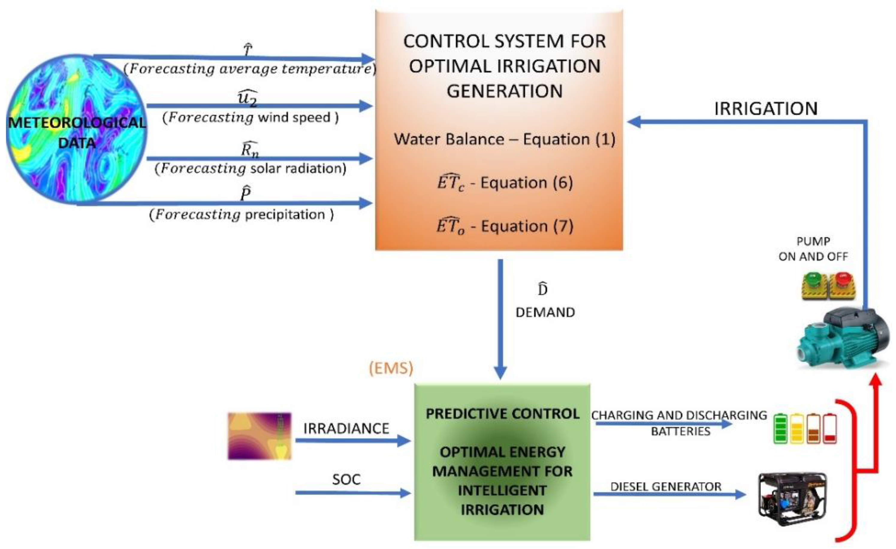
The proposed smart irrigation system considering optimal energy management with model predictive control MPC is shown in
Figure 3. It contains two stages. The initial stage focuses on obtaining the daily irrigation demand profile in a smart way through an expert system. This system is programmed to automatically obtain the daily moisture by means of the water balance, i.e., the water gain and loss in the root zone of the crop by means of Equation (1), for which the forecasted data of one day of precipitation
are needed as water input to the system. Similarly, it is necessary to know the water losses that occur in the crop by evapotranspiration. Using Equation (6), the evapotranspiration of the crop (
is determined and by means of meteorological data the referenced evapotranspiration is obtained with Equation (7). The energy demand is the result of the irrigation time for the daily turning on of the pumps throughout the day, this demand profile obtained is transmitted to the next stage which is called energy manager system (EMS) of the microgrid for the irrigation system; in this stage an optimization problem is solved and is responsible for the efficient management of the energy system to determine the energy needed to turn on the water pump, taking advantage of renewable resources for power generation. In this second stage (EMS), the availability of energy from the hybrid energy system formed of photovoltaic panels, storage systems and a diesel generator is guaranteed.
3.1. Expert System for the Generation of Optimal Irrigation—(First Stage)
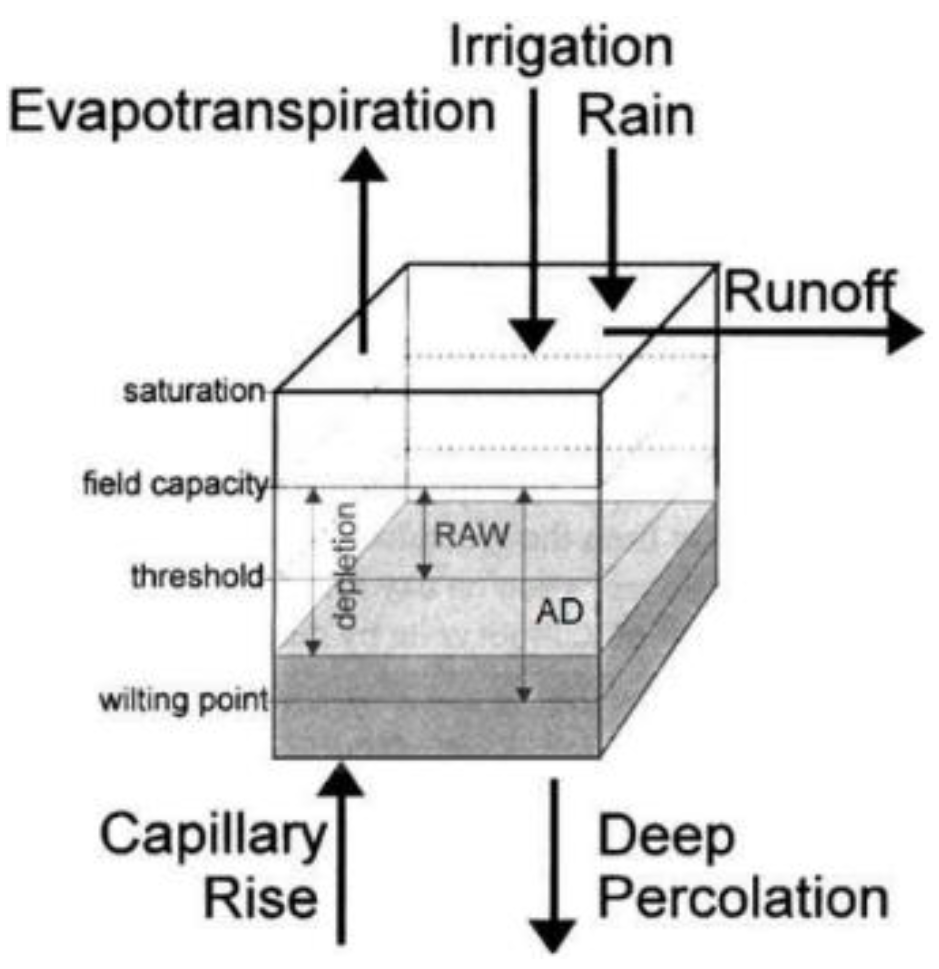
In order to guarantee optimum irrigation, we start with the study of the type of soil and the knowledge of its characteristics that help to maintain sufficient moisture for the crop without exceeding the limits of the field capacity and permanent wilting point. The analysis of the water balance is analyzed daily throughout the crop, the limits depend on the depth of the roots and how much water was contributed to or removed from the crop.
The upper part of
Figure 3 shows the forecasting data needed to determine the optimum irrigation (average temperature
, wind speed
, Solar radiation
and precipitation
), irrigation is automatically determined by an automatic expert system, which executes the following steps: (i) meteorological data and prediction models with a control horizon of one day during the cultivation time are obtained to determine the reference evapotranspiration
with Equation (7); (ii) the expert system determines the crop evapotranspiration (
) in one day with Equation (6), which depends on the value of the crop coefficient (
) in its different growth stages, determining the amount of water consumed or removed in the root zone; (iii) by means of the water balance of Equation (1), the soil moisture at the end of the day is known, thus determining the need for irrigation by means of the input of forecasts involved in the water balance.
In the automatic expert system, the lamina at the field capacity () of the plants is determined by Equation (2), which depends on the depth of the crop root ( and the bulk density of the soil . The lamina at field capacity is the maximum limit of water required in the crop and at this level water is optimally absorbed. The lower limit is lamina at permanent wilting point (); at this point the amount of water adheres only to the soil particles, which makes it impossible for the plant to obtain water and would generate water stress; therefore, to prevent the crop from reaching this point, the water content is determined at a suitable threshold (), which results from the sum of the value of with , thus preventing the water content at the root from reaching .
The irrigation required each day occurs when
, i.e., when the initial soil moisture
is less than or equal to (
), it is necessary to provide water to the crop, and the system has the capacity to automatically determine the necessary amount of irrigation lamina (
) by means of Equation (8), where the irrigation lamina (
) must be less than the field capacity lamina
, and the forecasted precipitation
is also taken into account to determine the amount of effective irrigation lamina (
, so that the crop does not suffer soil saturation.
Once the water requirement of the crop is determined, the gross or total irrigation lamina is determined to ensure sufficient penetration of water in the root zone, by Equation (9), since not all the water will be consumed by the plant, it is, therefore, necessary to apply a greater amount of water in irrigation with respect to the efficiency of the irrigation system [
28].
In Equation (9), is the gross lamina in , is the required irrigation lamina in and is the efficiency of the irrigation system.
To determine the all-day demand, the switch-on time of the pump is obtained by Equation (10) [
30].
In Equation (10), is the irrigation time in hours and is the average rainfall of the system.
According to the irrigation time, the necessary electrical demand for the day is obtained by multiplying the irrigation time with the pump power, thus sending the forecasting or necessary demand for the whole day to the next stage, which is in charge of supplying electric power with the optimal and efficient management of the pump start-up throughout the whole day.
3.2. Microgrid Controlled by Energy Management System (EMS) for Irrigation System (Second Stage)
The energy consumption to achieve smart irrigation can be supplied by a microgrid, which requires optimal management. When different isolated energy sources can be managed to supply energy in a coordinated and reliable way, the microgrid is composed by a diesel generator, solar panels and a battery energy storage system (BESS).
The second stage consists of the integration of smart irrigation with optimal energy management for the proposed microgrid. The operation of pumps are driven by generation units such as batteries, photovoltaic power or diesel generator.
The control is constituted by an optimization problem that, by means of the objective function of Equation (11), minimizes the diesel generation cost
, cost for energy not supplied
and cost for solar discharge
in order to take advantage of the solar energy and always preserve the useful life of the batteries. The total costs are obtained by multiplying the cost of generation by technology by the power generated by each unit as the diesel generator power
, which is presented when the optimizer detects that the available energy from the batteries or solar generation is not able to supply energy to the system. The power not supplied (
) occurs when the three energy sources present in the system are not able to meet the required demand. The solar curtailment power
occurs when the solar power is greater than the electrical demand.
The optimization problem is subject to equality and inequality constraints, referring to the generation units involved in the energy system.
The energy system consists of a battery energy storage system (BESS), which operates in discharge mode when it provides energy to the system and in charge mode when the batteries are recharged, being part of the energy consumption.
The first equality constraint is the energy balance, which is represented in Equation (12). The energy system needs to satisfy the energy balance, where the sum of the energy generated by the solar panels (
), the diesel generator
and the battery power in discharge mode (
), is equal to the sum of the electrical demand of electronics devices
, electrical demand to water pump (
, the solar dump power
, the unsupplied power and the battery power in charge mode (
.
The diesel generator has min power,
, and max power,
, operating limits, which are multiplied by a binary variable
. The binary variable decides whether to start the diesel generator or not and the diesel generator limit constraints are expressed in Equation (13).
The BESS model considers two operating modes: loading or unloading. For each mode, an equal loading and unloading efficiency coefficient
is considered. Equation (14) gives the available energy of the BESS at the first instant
, which is equal to the initially available energy
. The available energy of the BESS can start at a certain percentage, then the energy contributed by the BESS when in charging mode is subtracted and finally the energy of the BESS when in discharging mode is added, which is shown in Equation (14).
Equation (15) represents the point when the energy of the BESS starts to respond dynamically after the initial condition.
The available battery energy is less than or equal to the installed battery power
represented in Equation (16), the model requires the state of charge (
SOC), which estimates the amount of battery energy represented in Equation (17), and through the BESS usage policies limits the charging and discharging of the BESS, thus lengthening the BESS lifespan expressed in Equations (18) and (19).
The binary variables or optimization variables
take the value of zero or one to define the state of the BESS, so as to not turn on the BESS to charging or discharging mode at the same time, as defined by Equation (20).
The constraints represented by Equations (21) and (22) estimate the limit of the BESS power in charging and discharging mode.
The model solar generator power
is estimated by panel efficiency, inverter efficiency
with panel area
, number of panels
and irradiance
, expressed by Equation (23).
It must be ensured that solar dumping power
is less than solar generation power
, as represented by Equation (24). This ensures that maximum utilization of the solar resource is achieved.
4. Results
This section presents the results obtained by the application of the smart irrigation system, considering the proposed optimal energy management with predictive control. For the irrigation modeling, the meteorological data forecasts relevant weather for crops on daily basis, the acquired data being temperature, solar radiation, wind speed, relative soil moisture and precipitation. These records are obtained from the ‘POWER Single Point Data Access’ (
https://power.larc.nasa.gov/data-access-viewer/) accessed on 11 August 2022, which provides solar and meteorological datasets from NASA research to support renewable energy, building energy efficiency and agricultural needs. The obtained climatological data were recorded in an hourly computational database from July 1 through August 29, totaling 60 days, which corresponds to a full growing period of the alfalfa crop.
To determine the reference evapotranspiration, a database was programmed and by means of the FAO Penman–Monteith equation (Equation (7)) the daily reference evapotranspiration was determined in the Excel add-in HF Irrigation.
The solar irradiance data were obtained from ‘POWER Single Point Data Access’ records, the irradiance data are used for the EMS with a daily prediction horizon totaling 24 samples per hour, which allows the optimization of energy management using the FICO® Xpress Workbench software, as it has the ability to solve optimization problems.
4.1. Case Study
The present research was carried out by the sizing of a plot of 1173
in Ecuador, located in the province of Cotopaxi, in the canton Latacunga, parish Ignacio Flores, with a latitude of −0.935061 and longitude of −78.603145, where the terrain is sandy loam and the reference crop is alfalfa [
19].
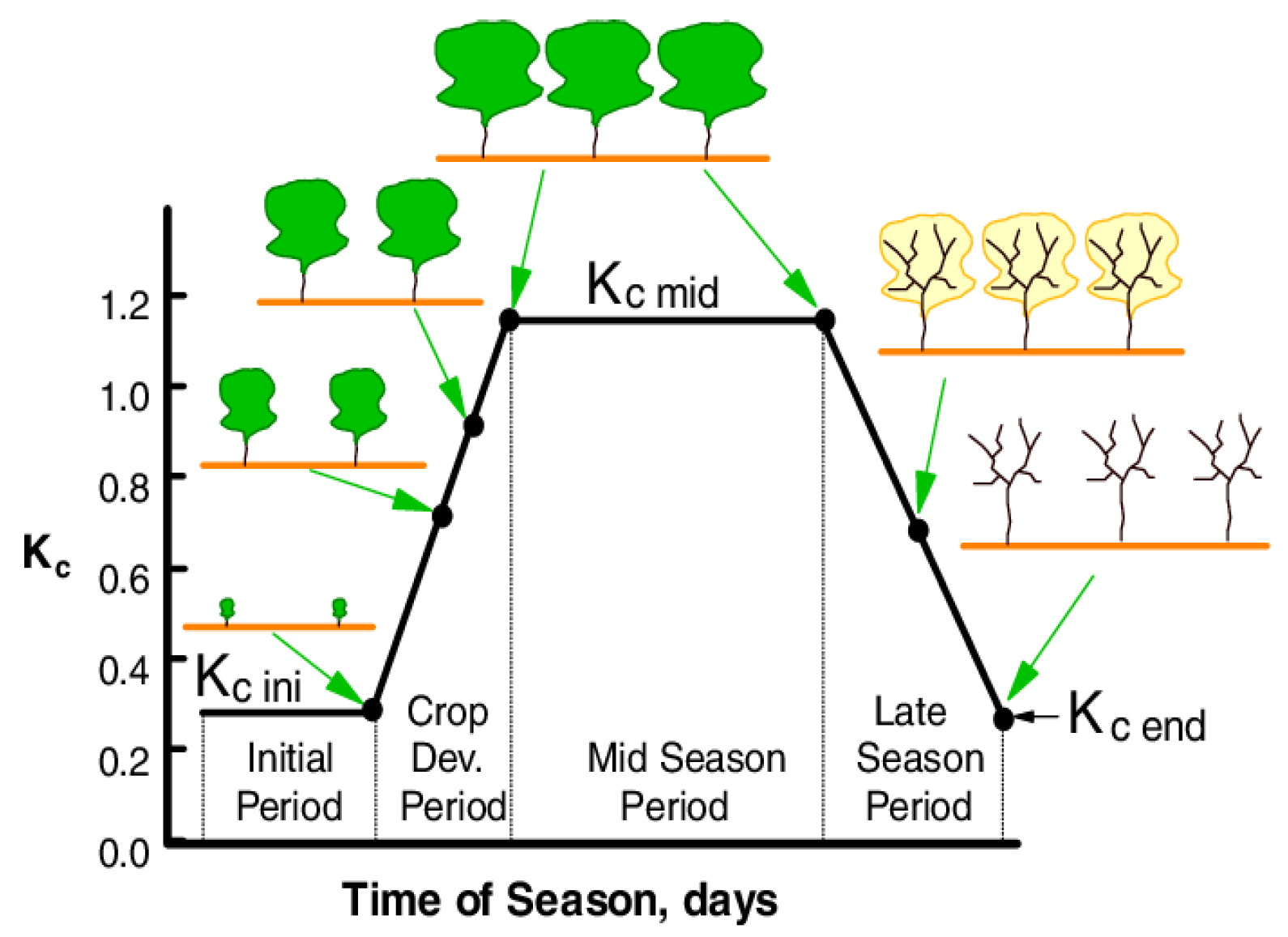
The crop in this research is alfalfa and, according to FAO-56 [
26], alfalfa development time is 60 days, distributed over 10 days in the initial stage, 20 days of development, 2 days in the middle stage and 10 days the final stage, with its corresponding crop coefficient of
,
and
= 1.15.
The soil properties are represented in
Table 1, which indicate the values used in the development of the research.
The required irrigation lamina or net irrigation lamina represents the amount that can be easily extracted by the plants, according to Equation (5). Where the average fraction of the total water available in the soil is the factor that indicates the sensitivity of the crop to a threshold, whether it is very delicate or of high economic value, such as vegetables or flowers, this factor adopts a value between 0.3 and 0.4 (30–40%) [
30].
The irrigation system consists of 12 sprinklers with a spacing between sprinklers
of 10 m, a pressure of 20 PSI and a flow rate of 1.1 GPM. With Equation (25) the average rainfall of the system of
is obtained [
19].
The energy consumption of each piece of equipment that makes up the smart irrigation system is detailed in
Table 2:
Table 3, below, details the technical data of the hybrid energy system of the sources available for energy management.
4.2. Irrigation Technique to Evaluate and Compare
Three irrigation techniques were evaluated and compared: (i) traditional irrigation, (ii) technified irrigation, and (iii) proposed smart irrigation.
4.2.1. Traditional Irrigation
Traditional or empirical irrigation is an intuitive irrigation, which applies water resources with a pump and by means of a sprinkler system, without considering technical parameters. Using this irrigation method, the pump is turned on for one hour daily (at night), throughout the whole growing period of 60 days of the alfalfa crop.
4.2.2. Technified Irrigation
The type of technified irrigation is based on an agronomic design, the water requirements of the crop are determined by calculating the irrigation calendar, taking into account the duration of the 60-day crop, corresponding to the alfalfa growing period from July 1 to August 29. By means of the meteorological data ‘POWER Single Point Data Access’ of the NASA and the extension of Excel HF irrigation, the reference evapotranspiration in the month of July is obtained.
The crop coefficient
Kc of alfalfa, with the duration of each stage and root depth, is shown in
Table 4.
Equation (26) determines the frequency of technical irrigation that results from the division of the lamina of readily available water from the crop evapotranspiration
.
Table 5 determines the irrigation schedule according to the irrigation needs, taking into account the reference evapotranspiration
; crop coefficient
; crop evapotranspiration
, according to Equation (6); irrigation frequency from Equation (25); irrigation numbers; gross lamina from Equation (8) and irrigation time
).
4.2.3. Proposed Smart Irrigation
The proposal uses the daily water balance to determine the amount of water in the root zone and, through irrigation, to modify the amount of water, respecting the limits that must be kept lower than the field capacity (
) and higher than the permanent wilting point
. The balance is based on the input and output of water in the root zone, and the proposed system in
Figure 3 of the first stage is applied to generate the optimal daily demand.
The initial moisture is taken into account from the date of planting or when the first irrigation performed; the precipitation is the rainfall that occurs per day and the amount of water it brings to the soil; the irrigation is the amount of water that the controller will bring, depending on the initial moisture and limits; the crop evapotranspiration depends on climatic conditions such as wind, solar radiation, average temperature and relative soil moisture to obtain the reference evapotranspiration and, finally, the crop coefficient depends on the stage of development of alfalfa.
The proposed smart irrigation determines the upper limit or maximum moisture limit, which is the lamina at field capacity with Equation (2) and the minimum limit of water content at a suitable threshold (). In this way, the plant does not suffer water stress and does not reach below the point of permanent wilting lamina . These limits depend on the depth of the root until the first cut, then the root maintains its depth, keeping these limits constant. is the irrigation required when the initial moisture is less than or equal to .
Table 6 shows the irrigation schedule applied to the proposed smart irrigation during the first 10 days in the intermediate stage of the crop. From day 31 to day 38 there is no precipitation
, therefore the system generates irrigation
.
The maximum irrigation input is 7.49 mm since a maximum irrigation time of 4 h per day is considered.
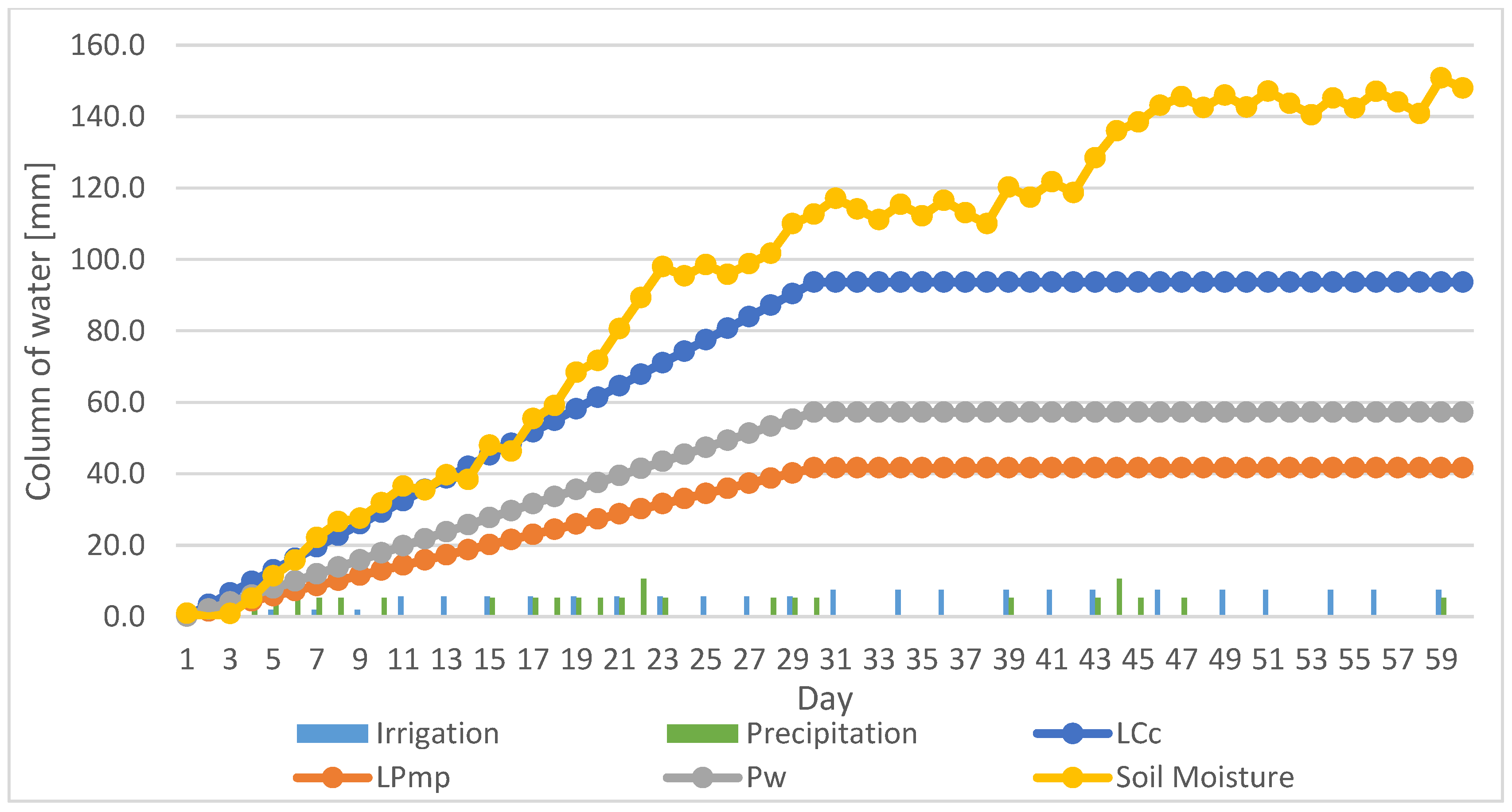
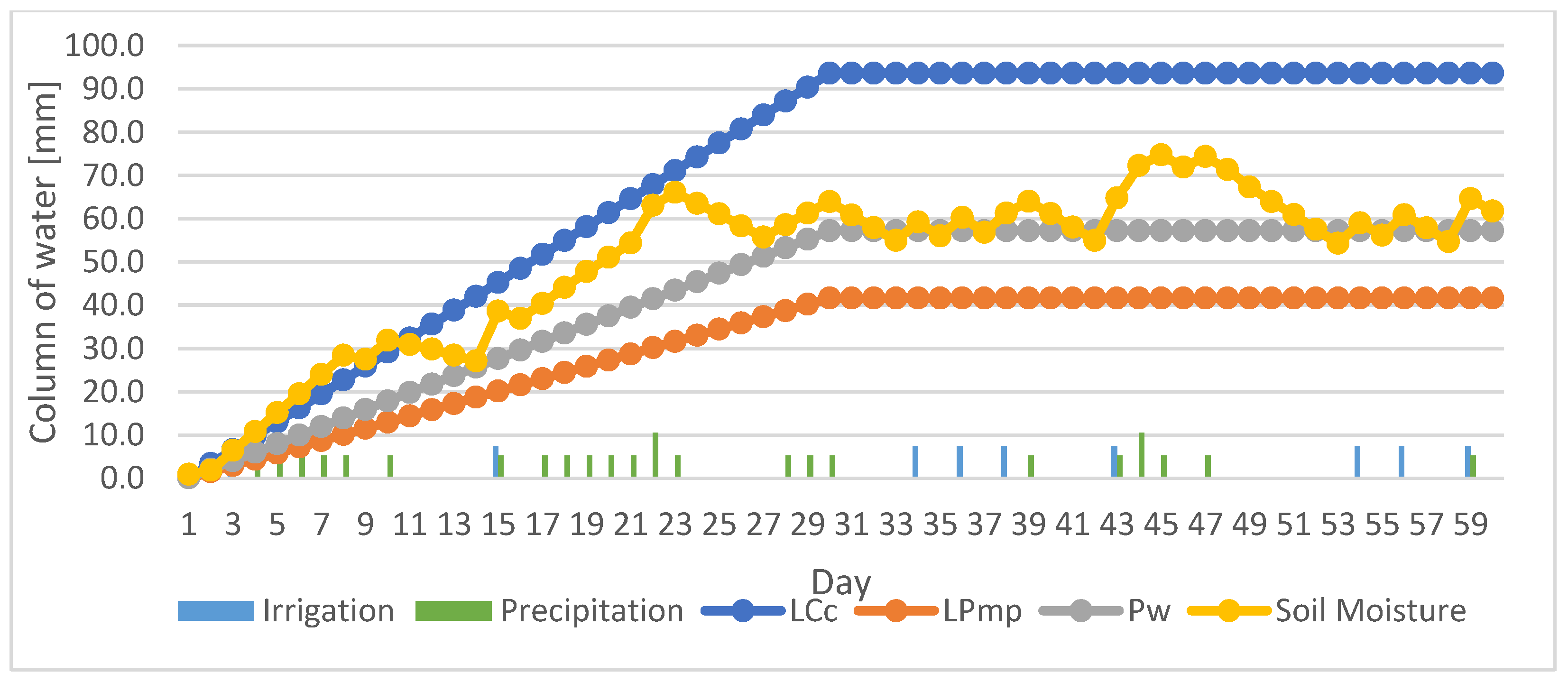
4.3. Moisture Analysis When Evaluating the Different Irrigation Techniques
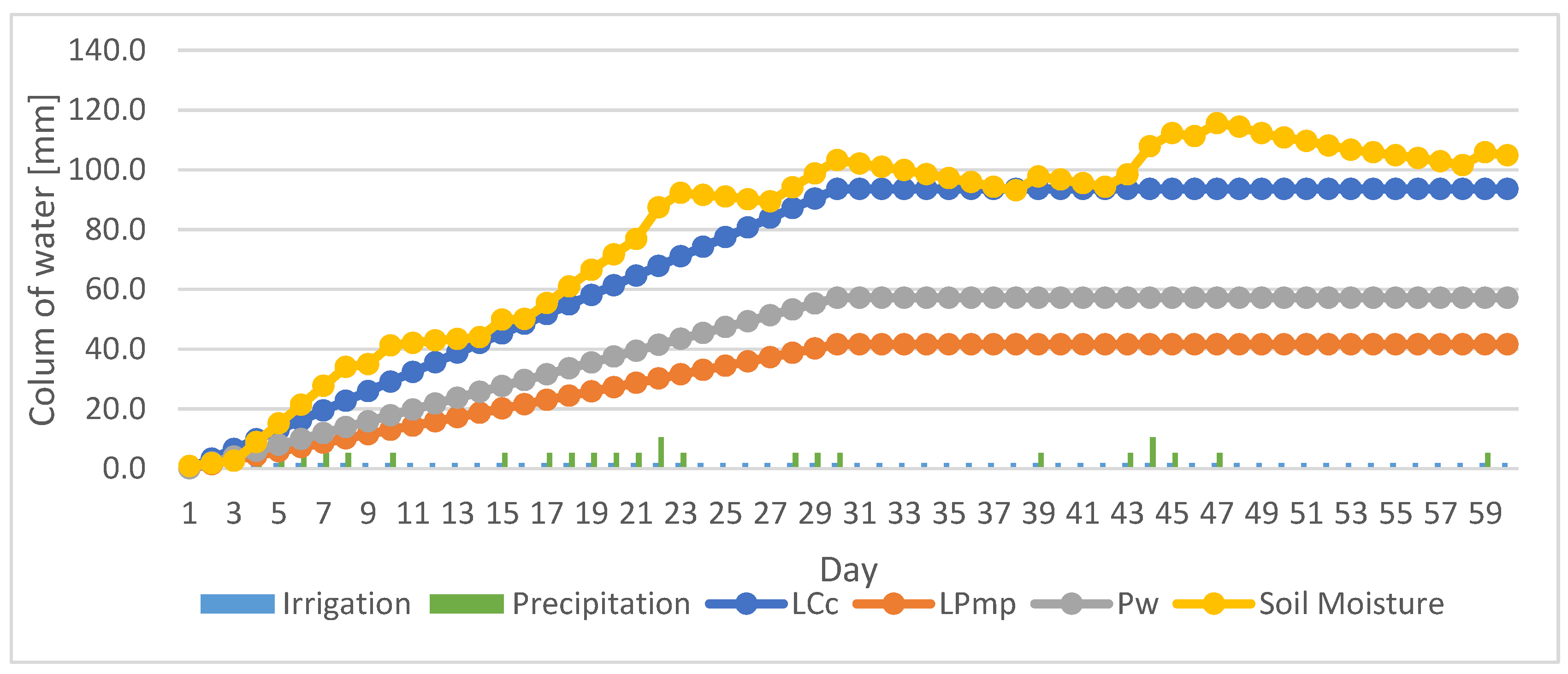
In this section the three irrigation techniques are compared and the moisture that the crop will have is analyzed to verify that it does not exceed the moisture limits. In
Figure 4,
Figure 5 and
Figure 6 the yellow line representing the moisture level at the end of each day is identified, the blue line represents the maximum water content level at field capacity, the orange line is the minimum level that the crop can obtain and, finally, the gray line is the lower limit
and the readily available water (RAW). The abscissa axis (y) represents the water sheet or moisture in the root zone and the coordinate axis (x) represents the development of alfalfa in a 60-day cycle.
Figure 4 shows the moisture with traditional irrigation where the moisture curve,
, represented in yellow color, exceeds the curve
indicated in blue color, where it can be observed that there is an excess of water in the different stages of the crop during the 60 days, and the excess water is lost by runoff or by deep percolation.
Figure 5 shows the soil moisture in the technified irrigation technique, carried out by means of an agronomic design, when observing the soil moisture,
, represented by a yellow curve, it is evident that there is an excess of water resources because it exceeds the blue curve
throughout the whole period of the crop, but this excess water is lost and is not usable, so there is a waste of water resources.
The third irrigation technique is the proposed smart irrigation that uses the daily water balance with a maximum irrigation time of 4 h, shown in
Figure 6. The soil moisture,
, is represented by a yellow curve and is maintained within the range of the allowed limits without causing water stress or saturation of the soil due to excess water
When comparing and analyzing
Figure 4,
Figure 5 and
Figure 6 of the three irrigation techniques, it should be noted that the smart irrigation proposal maintains the necessary moisture without causing water stress or soil saturation due to excess water, while the traditional and technified irrigation techniques produce water losses, while the smart irrigation technique makes optimal use of the water resources.
4.4. Economic Analysis of Irrigation Techniques
Once the irrigation performance of the crop has been evaluated, the economic cost of irrigation is now analyzed, for which two scenarios are analyzed and applied to the three irrigation techniques.
4.4.1. Scenario 1
This scenario is applied to the three irrigation techniques where the only source of energy to supply the electrical demand for irrigation is a diesel generator, whose tank capacity is approximately one gallon with an estimated autonomy of two hours. This scenario is used since diesel generators is currently used in many rural areas with crops, because the electrical grid does not supply energy to different crop areas in the rural regions.
To determine the costs for diesel generation in the three irrigation techniques, the value of diesel fuel in Ecuador is used, with a value of USD 1.90 per gallon. The number of gallons to be used in each technique is determined by using Equation (27) and the cost generated by diesel consumption by Equation (28)
Table 7 summarizes the cost generated by each irrigation technique, considering the irrigation times during the 60 days of the crop, the total time in the traditional irrigation is 60 h, in the technified irrigation the total irrigation time is 83 h, while in the smart irrigation method proposed the irrigation time is 37 h, as determined by Equation (10), the irrigation time resulting from the quotient between the gross lamina
and the average rainfall of the sprinkler irrigation system
.
Analyzing the costs generated in
Table 7 for each irrigation technique, it is shown that the traditional irrigation would generate a cost of USD 57, the technified irrigation generates a cost of USD 78.85, while the proposed smart irrigation cost is USD 35.15 during the cultivation time. Therefore, it can be concluded that the cost for technified irrigation and traditional irrigation is high compared to the proposed smart irrigation, which is the most economical and also allows the compliance with the best technical characteristics, regarding irrigation.
4.4.2. Scenario 2
The proposed smart irrigation, in conjunction with energy management, requires 37 h of irrigation, of which the days that the pump spends more time on is 4 h, performing energy optimization and thus not using the diesel generator to turn on the pump and obtaining zero cost for power generation. Our proposal, because it takes the future into account and is based on it, can make decisions based on optimal solutions and always takes the most optimal on and off point for the pump, whether there is sun or not, and thus it will always be the most efficient.
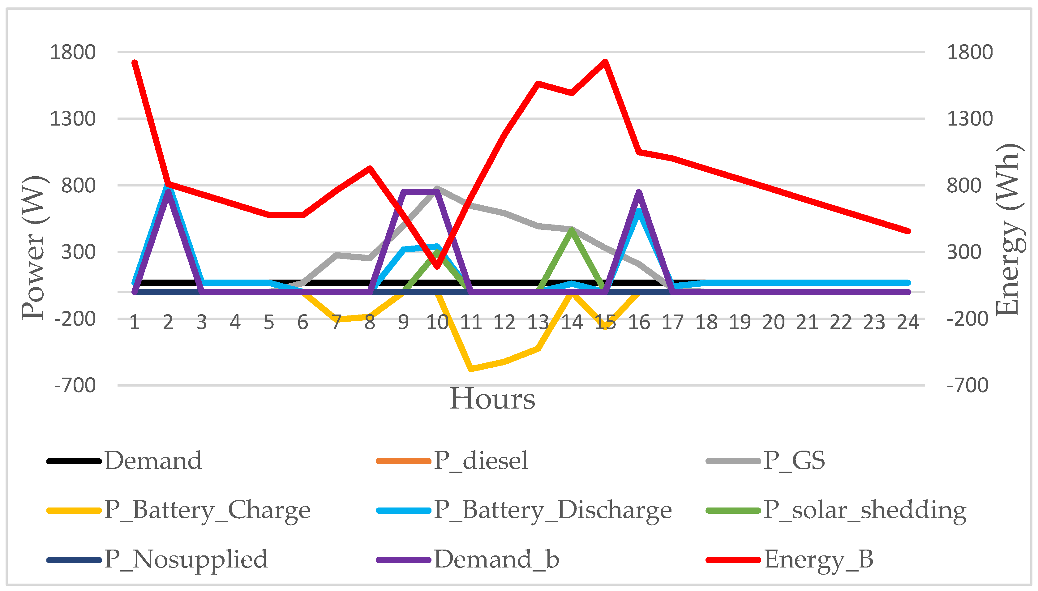
4.5. Analysis of Energy Management in the Three Irrigation Types
Figure 7 shows the energy management with the proposal of a predictive control, based on MPC models with a control horizon of one day for the proposed optimal irrigation, where the energy or energy demand of the pumps (Demand_b) sent by the expert system is the 4 h turn-on, represented by the purple line, the optimizer decides the pump start-up time automatically and thus optimizes the sources that provide energy to the system, identifying the best time for the batteries to operate in charge or in discharge mode. The available energy of the BESS system (Energy_B) is represented by the red curve. It can be observed that there is no use of the diesel generator (P_diesel), i.e., it does not generate cost in the system, keeping the brown curve at zero. The solar power (P_GS), represented by the lead curve, indicates that it is used to recharge the batteries when conditions are more opportune. The yellow line represents when the batteries are in charge mode (P_Battery_Charge), and the light blue curve indicates when the BESS system is in discharge mode (P_Battery_Discharge), while the blue curve represents the energy not supplied (P_Nosupplied), which is kept at zero, i.e., the system is maintained with the necessary energy all the time. It can also be observed that the green curve is the solar shedding (P_solar_shedding) the excess solar energy when more energy is produced than is demanded.
After reviewing the energy consumption with the irrigation techniques of the crop in Scenario 2, the curves of energy consumption without management can be analyzed, i.e., the pumps are turned on according to a fixed schedule and the system must supply energy whatever the source (traditional irrigation, technified irrigation), whereas in the proposed irrigation with optimal energy management, the optimizer has the flexibility to see the most appropriate time to turn on the pump, taking advantage of solar energy and batteries, to avoid the ignition of the diesel generator as much as possible.
There are no proposals describing optimal irrigation simultaneously with the energy management used to supply the electrical irrigation demand. However, a comparative analysis was performed concerning a smart irrigation system proposed in [
31], in which the control system is based on fuzzy logic. The ignition pump was analyzed in order to establish the differences found in our proposal regarding energy consumption. In [
31], the water pump powered up for 7 h of growing period (three days). Compared to our proposed smart irrigation, the pump powers up for 3 h during the growing period, achieving a good performance in the crop. The powering up of the pump is related to the cost of energy consumption. Therefore, [
31] presents a higher cost. Moreover, unlike [
31], our proposal includes the management of a microgrid based on renewable sources.
5. Conclusions
In this research, three irrigation techniques were evaluated and compared, the first one known as traditional or empirical that is applied by many farmers. The second one was called technified irrigation, which applies agricultural knowledge to create the irrigation schedule, and, finally, the smart irrigation proposed in this work. The smart irrigation proposal plans irrigation automatically and intelligently, considering energy management. When comparing the three techniques, it can be observed that traditional irrigation and technical irrigation exceed the moisture limit range, which indicates a waste of the water resources that can generate soil saturation, damaging its maximum growth. Whereas with the intelligent irrigation proposal, the moisture is within the limit band, which benefits plant growth and avoids wasting water.
The smart irrigation system proposed, when compared to traditional irrigation, decreases diesel consumption by 38.4% and saves 55.42% compared to technified irrigation; by implementing the EMS of the microgrid, the cost for electricity generation creates a saving of 100% compared to technified irrigation. Being more economical, the proposed smart irrigation system optimizes the efficient use of water in the crop and maximizes the use of renewable resources in energy management.
Finally, the smart irrigation proposal generates the irrigation hours in a crop and supplies the required electrical demand through the use of a microgrid based on renewable resources, at the same time that the environment is respected. The pump on/off system is according to the technical and optimal irrigation conditions. Also, the proposed determines the battery operation set points by taking into account the limitations of the SOC. If necessary, the diesel generator power is defined. The decisions made by the EMS maximizes the use of natural resources. This proposal ensures that water resources is not wasted by keeping the moisture in the desired range, allowing for optimal crop growth and an uninterrupted power supply.


