Jointing Principles in AMC—Part 1: Design and Preparation of Dry Joints

Abstract

The study described in this contribution contains a fundamental strategy to select geometries for dry joint profiles in 3D-printed concrete constructions. A database, here called the ‘joint catalogue’, contains a variety of joint types adapted from timber, steel, and bionic connections. Weighting factors and different criteria evaluate and score the various joint profiles (e.g., manufacturability, duration of manufacturing, and mechanical behaviour). Therefore, an algorithm sums up the scores leading to the preselection of better suitable profiles. The preselected joint profiles were afterwards analysed by the finite element method, determining the load capacity of the joint in a unit specimen. According to the joint catalogue, a smooth, triangular, truncated cone and arc joint profile appeared to be the optimal combination for dry joints in additive manufacturing of construction (AMC).

1. Introduction

The modern world is changing faster than ever before, and the civil engineering field is no exception to that. Therefore, the requirements for the construction industry are increased speed, sustainability, and being digital to remain economical and become more efficient. With its long duration of planning, high carbon emissions, and questionable digitalisation, the construction industry faces formidable challenges to become less bureaucratic, more resource-efficient and intelligent. In that sense, new digital technologies like building information modelling (BIM) and 3D-concrete printing are gaining increased popularity. Three dimensional (3D) concrete printing, or additive manufacturing in construction (AMC), can take place on-site as well off-site [1,2,3,4]. For on-site printing, in other words, printing at the construction site, the dimensions of the entire components are limited to the size of the 3D-concrete-printer according to the used method. In a recent work, Xiao et al. [5,6] described some examples for different methods in the case of large-scale 3D printing systems. However, these large-scale 3D-printing systems have their limitations, not in the pure scale of the component, but in the environment. For example, engineering structures like bridges, silos, towers cannot be printed in one single piece because the surrounding area is not usable or available. Therefore, the components must be separated into smaller pieces and merged by using joints. Off-site printing, i.e., printing in a prefabrication plant, limits the dimensions of the components to ease the transportation. To deal with this limitation due to the size of the printed components, either it is possible to optimize the topology of a layout so that a building does not require large components or to divide bigger elements into smaller elements and reassemble them with joints on the construction site. The jointing of several components is required for off-site printing and on-site printing as well. This shows the relevance of the jointing in AMC.

Conventional jointing principles are nowadays match-cast and grouted joints [7,8]. Match casting means that one joint of a structural element serves as a formwork for the other half of the pair (side). In this case, a conventional formwork is still required to manufacture the joint of the original structural element. As match casting still requires formwork, the procedure might only be efficient for linear structural components. Furthermore, shrinkage of the joint profile might lead to inaccuracy of its geometry causing difficulties in fitting and load transfer/distribution [9]. On the other hand, grouted joints require even more attention in manufacturing because they do not only need formwork for the structural elements but also grouting for the joint. This sort of complicated and sometimes inaccurate manufacturing process could be listed as a disadvantage of this technique.

In 2017, the first post-tensioned pedestrian bridge composed of extruded additive manufactured (AM) concrete segments and connected by grouted joints was built in the Netherlands. Compared to the conventional in-situ concrete construction method, time and cost savings were achieved regarding formwork, and the fabrication and installation of the reinforcement cages [10]. The manufacturing might have been more efficient if dry joints instead of grouted joints had connected the construction elements. In this case, the task of grouting the jointed elements could have been saved.

One of the main advantages of the AM process (shotcrete, extrusion, and particle-bed) is that the production of concrete segments is formwork-free. However, this advantage might disappear if the dry joint between the concrete segments itself requires formwork. “Zero tolerance” dry joints are manufacturable via match-cast [11], CNC-milled (CNC: Computerized Numerical Control) high-precision formworks [11,12], high-pressure water jet cutting (WJC) [13] and CNC-concrete milling technology [14]. Match-cast and high-precision formworks still require at least one formwork, while WJC and CNC-concrete milling are formwork-free technologies. Notwithstanding, WJC is a 2D cutting process, limiting the possibility of manufacturing complex joint geometries like truncated cones or cams into concrete components. High-pressure water jet cutting can be utilized only for cutting thin and planar components. Hence, the joint’s robotic finishing with CNC-milling is the most capable technique for AM segments.

This new technique of manufacturing an indented joint profile into a concrete element, so-called ‘Subtractive Post-processing’, utilizes, e.g., CNC-milling or CNC-sawing for producing various concrete dry connections. In this process, the milling tools or saw blades are connected to a multi-axle robot (see Figure 1a). Generally, the subtractive post-processing starts once the concrete is hardened. However, CNC-operation on hard concrete (Figure 1c) demands a high amount of energy and causes faster ageing of the milling/sawing tools, while operation on fresh concrete (Figure 1b) can reduce the consumed energy. The downside of processing fresh concrete is the lower manufacturing accuracy, as the fresh concrete’s scarce stability (green-stand strength) might lead to undesirable deformations. Therefore, an additional laser scanner is linked to the robot to monitor the path of the robotic CNC-arm and consequently the concrete geometry, tracking the deformation of the printed concrete elements toward live adaptions [15] to fit the attained geometry of the element.

2. State of the Art and Research Outline

Dry joints performed with CNC-milling were successfully used by the construction company Max Bögl in the serial production of precast high-strength segmental post-tensioned concrete towers for wind turbines [14]. Based on this experience, the arch of a tied-arch bridge [16] and a prototype for a segmental ultra-high performance concrete railway bridge [17] were built. The segments were produced conventionally in all cases, and the joints were milled. The CNC-milled joints were executed as smooth dry joints, and the flatness of the joint end faces was limited to 0.1 mm/m. These high accuracy requirements were determined based on tests because normative regulations are still missing.

The joints between the segments could be weak points and hence decisive for the structural design. Investigations of the load-bearing capacity of dry joints, along with segmental components with dry joints made of normal concrete and produced conventionally, were carried out, e.g., by [18,19,20,21]. An overview of the tests carried out on normal concrete can be found in [22]. Based on these investigations, a calculation approach for determining the load-bearing capacity of normal strength dry joints was proposed [22]. Furthermore, a new computation method for the parametric evaluation of joint geometries by machine learning techniques was addressed [23].

Recent investigations dealt with the load-bearing capacity of dry joints and segment components with dry joints made of ultra-high performance fibre-reinforced concrete (UHPFRC) [24,25,26]. The investigations show that the load-bearing capacity of UHPFRC dry joints differs from normal strength dry joints. In former studies, new joint geometries were proposed and evaluated [27,28]. Nonetheless, the match-cast process produced all the test specimens of these investigations.

For this study, as part of a tandem research project funded by the German Research Foundation under TRR 277, subproject C05 investigated the jointing principles in Additive Manufacturing in Construction (AMC). The subproject C05 contains four consecutively structured working packages WP1–WP4 (Figure 2). The WP1 aims to design and select joints profiles for 3D-printed elements. A set-up database (joint catalogue) is used, containing the main imaginable joint profile types and geometries taken from timber, steel and bionic connections. It also contains evaluation criteria, weighting factors, and an algorithm to evaluate the gathered joint profiles regarding the applicability for 3D-printed concrete elements. The algorithm then, proceeds to select four joint profiles to be further analysed by packages WP2, WP3 and WP4. In WP2 and WP3, the goals are to understand the load-bearing behaviour under compression and shear by numerical simulation and experimental testing, while in WP4, the results of the previous packages are used to design, simulate and test a 3D-printed, and via dry joints connected component.

Considering the process described above, this paper shows the results of WP1, i.e., which joint profile types are associated, evaluated by various criteria, and selected by the algorithm. Furthermore, this contribution deals with the preliminary investigations for the subtractive post-processing required for manufacturing the specimens for experimental investigation in WP2–WP4.

3. Joint Catalogue

The joint catalogue is a database that contains an enormous variety of joint configurations. The examples of the joint profiles come from segmental concrete constructions, which can be adapted from timber, steel or bionic structures. Regarding the impossibility of investigating all joint profiles numerically and experimentally, along with the disability of the normal analysis in considering different aspects of the dry joints, a preselection based on the engineering judgment is necessary. In principle, various criteria are used for the evaluation of each joint profile, and then, subsequently, the joint profile with the highest score, i.e., best evaluation is selected for further investigation. The evaluation is based on a scoring system and weighting factors for each criterion considering the main goals of subproject C05.

Table 1. Excerpt of joint catalogue.

Excerpt of Joint Catalogue
Category	Line-Shaped	Point-Shaped	Mesh-Shaped
Joint profile	Triangular	Pyramid	Smooth
	Saw tooth	Truncated Pyramid	Napped
	Trapezoid	Truncated Pyramid	Lego
	Dovetail	Cross	Chequerboard

shows an excerpt of joint profiles in the catalogue, divided into line-shaped, point-shaped, and mesh-shaped. Every considered joint profile contains two parts, i.e., a female and male part. The goal of the first work package (WP1) is the selection of three to four joint profiles for further numerical and experimental investigation in the other work packages. The joint catalogue is, therefore, a preliminary tool to evaluate joints for concrete constructions.

3.1. Evaluation Criteria and Scoring

The evaluation criteria for joint profile selection are: manufacturability, anisotropic connectivity of a joint in a structure, detachability, duration of manufacturing, joint quality, compression strength, tensile strength, shear strength, torsional strength and failure mode. The comparability required a unit joint configuration. Therefore, the cross-section of all joints is $l_{\max } = b_{\max } = 100 \mathrm{mm},$ and the depth of the profile is $h_{\max } = 10 \mathrm{mm}$ (Table 1). Each evaluation criterion gives each joint profile a score based on assumptions made in the evaluation. The scoring lies within a range between zero and four, investigating and displaying the capability of each joint regarding one of the above-mentioned criteria.

Table 2. Overview of evaluation criteria and scoring in joint catalogue.

	Algorithm
	0	1	2	3	4	Weighting Factor
						1: less important 2: important 3: very important
Manufacturability	No possibility of manufacturability	Small possibility of manufacturability	Medium possibility of manufacturability	High possibility of manufacturability	Very high possibility of manufacturability	2
Description	Manufacturing of joint not possible: CNC, DP, FW, WJ, CS	Joint can partly be manufactured: CNC, DP, FW, WJ, CS	Joint is manufacturable: CNC, DP, FW, WJ, CS:	Joint can be easy manufactured: CNC, DP, FW, WJ, CS	Joint manufacturing is very easy: CNC, DP, FW, WJ, CS	CNC: milling DP: direct printing FW: formwork WJ: waterjet CS: circular saw
Connectivity	No connectivity	Small connectivity	Medium connectivity	High connectivity	Very high connectivity	2
Description	Radial. Axial, lateral	Radial. Axial, lateral	Radial. Axial, lateral	Radial. Axial, lateral Radial. Axial, lateral Radial. Axial, lateral	Radial, axial, lateral	radial: 90°-twistability axial: attachment lateral: insertion
Decomposability	No decomposability	Small decomposability	Medium decomposability	High decomposability	Very high decomposability	1
Description	Joint cannot be dismantled, demolition, detonation etc. necessary	Joint dismantling in very time consuming, demolition necessary	Heavy tools for decomposing a joint required	Light tools for decomposing a joint required	No tools for decomposing required	-
Duration	Very time-consuming production	Time-consuming production	Medium production speed	Fast production	Very fast production	2
Description	Joint surface $O_{\mathrm{j}}\ge 200 {\mathrm{cm}}^2$	Joint surface $O_{\mathrm{j}}\ge 160 {\mathrm{cm}}^2$	Joint surface $O_{\mathrm{j}}\ge 140 {\mathrm{cm}}^2$	Joint surface $O_{\mathrm{j}}\ge 120 {\mathrm{cm}}^2$	Joint surface $O_{\mathrm{j}}\ge 100 {\mathrm{cm}}^2$	-
	duration $t_{CNC}\ge 240\min /\mathrm{joint}$	duration $t_{CNC}\le 240\min /\mathrm{joint}$	duration $t_{CNC}\le 120\min /\mathrm{joint}$	duration $t_{CNC}\le 60\min /\mathrm{joint}$	duration $t_{CNC}\le 30\min /\mathrm{joint}$
Joint Quality	Insufficient joint quality	Inadequate joint quality	Average joint quality	Good joint quality	Very good joint quality	1
Description	Quantity of damageable edges > 20	Quantity of damageable edges $\le$ 20	Quantity of damageable edges $\le$ 15	Quantity of damageable edges $\le$ 10	Quantity of damageable edges $\le$ 10	-
	Length of damageable edges > 100 cm	Length of damageable edges $\le$ 100 cm	Length of damageable edges $\le$ 80 cm	Length of damageable edges $\le$ 60 cm	Length of damageable edges $\le$ 40 cm
Compressive Strength	No compressive stress transferable	Small compressive stress transferable	Medium compressive stress transferable	High compressive stress transferable	Very high compressive stress transferable	3
Description	Combination of surface and inclination of joint: $N_{Rd,tho}\ge 80 {\mathrm{cm}}^2$	Combination of surface and inclination of joint: $N_{Rd,tho}\ge 60 {\mathrm{cm}}^2$	Combination of surface and inclination of joint: $N_{Rd,tho}\ge 40 {\mathrm{cm}}^2$	Combination of surface and inclination of joint: $N_{Rd,tho}\ge 20 {\mathrm{cm}}^2$	Combination of surface and inclination of joint: $N_{Rd,tho}\ge 0 {\mathrm{cm}}^2$	-
Tensile Strength	No tensile stresses transferable	Small tensile stresses transferable	Medium tensile stresses transferable	High tensile stresses transferable	Very high tensile stresses transferable	1
Description	Tensile area: $f_{\mathrm{Rd},\mathrm{ct}}\le 20 {\mathrm{cm}}^2$	Tensile area: $f_{\mathrm{Rd},\mathrm{ct}}\le 40 {\mathrm{cm}}^2$	Tensile area: $f_{\mathrm{Rd},\mathrm{ct}}\le 60 {\mathrm{cm}}^2$	Tensile area: $f_{\mathrm{Rd},\mathrm{ct}}\le 80 {\mathrm{cm}}^2$	Tensile area: $f_{\mathrm{Rd},\mathrm{ct}}\le 100 {\mathrm{cm}}^2$	-
Shear Strength	No shear stresses transferable	Small shear stresses transferable	Medium shear stresses transferable	High shear stresses transferable	Very high shear stresses transferable	3
Description	Shear area: $v_{\mathrm{Rd}}\le 20 {\mathrm{cm}}^2$	Shear area: $v_{\mathrm{Rd}}\le 40 {\mathrm{cm}}^2$	Shear area: $v_{\mathrm{Rd}}\le 60 {\mathrm{cm}}^2$	Shear area: $v_{\mathrm{Rd}}\le 80 {\mathrm{cm}}^2$	Shear area: $v_{\mathrm{Rd}}\le 100 {\mathrm{cm}}^2$	-
Torsional Strength	No torsional stresses transferable	Small torsional stresses transferable	Medium torsional stresses transferable	High torsional stresses transferable	Very high torsional stresses transferable	1
Description	Torsional area: $T_{\mathrm{Rd}}\le 20 {\mathrm{cm}}^2$	Torsional area: $T_{\mathrm{Rd}}\le 20 {\mathrm{cm}}^2$	Torsional area: $T_{\mathrm{Rd}}\le 20 {\mathrm{cm}}^2$	Torsional area: $T_{\mathrm{Rd}}\le 20 {\mathrm{cm}}^2$	Torsional area: $T_{\mathrm{Rd}}\le 20 {\mathrm{cm}}^2$	-
Failure Mode	Four failure modes—no loads transferable	Three failure modes—at least one load type transferable	Two failure modes—at least two load types transferable	One failure modes—at least three load types transferable	No failure modes—all load types transferable	1
Description	Compression, tension, shear, torsion	Compression, tension, shear, torsion (at least one)	Compression, tension, shear, torsion (at least two)	Compression, tension, shear, torsion (at least three)	Compression, tension, shear, torsion	-

shows an overview of the evaluation criteria and the scoring.

The selection of a score between zero and four has been robustly calibrated by the evaluation criterion manufacturability of a joint, because it is one important topic in subproject C05 of TRR 277.

• Score 0: The joint profile is too complex, and no methods or tools are available for production.
• Score 1: The joint profile is still very complex, but modern tools like CNC-milling, or production methods like direct printing, make the joint profile manufactural. These tools can work three-dimensionally. Every joint profile that is manufactural with CNC is also manufactural with direct printing.
• Score 2: The next limitation of producing a joint profile is the formwork. A formwork might also be able to manufacture a complex joint, but then, the formwork itself requires manufacture, e.g., CNC-milling making the whole manufacturing process of the formwork sophisticated.
• Score 3: Besides CNC-milling, direct printing and formwork, less complex joint profiles might also be manufacturable by water jetting.
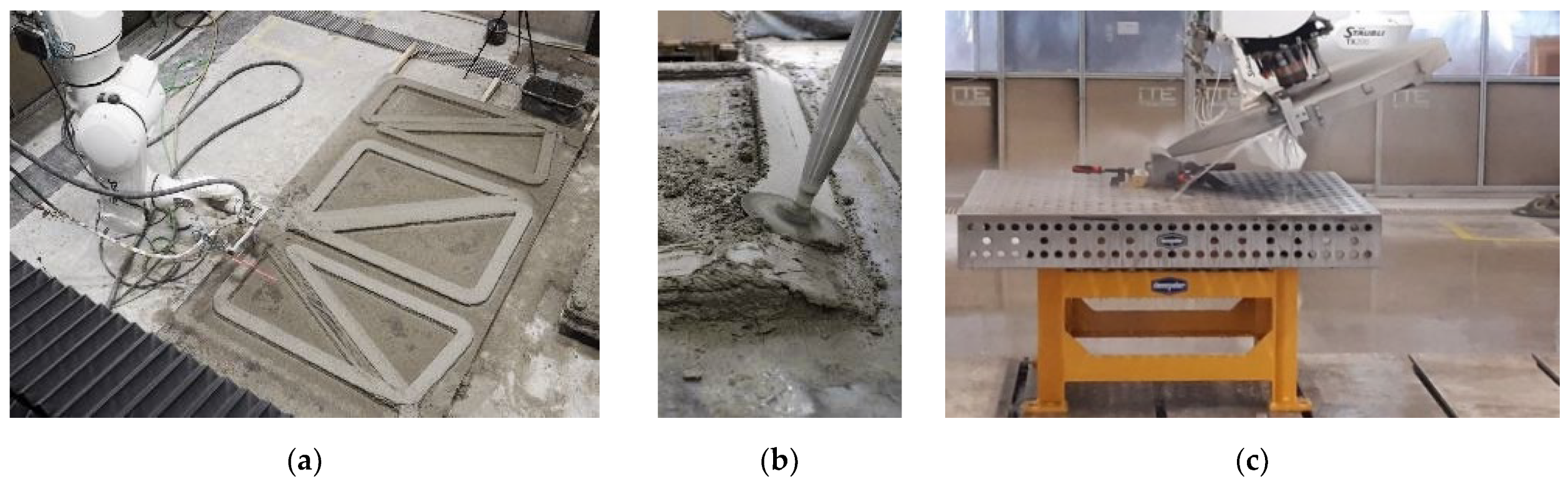
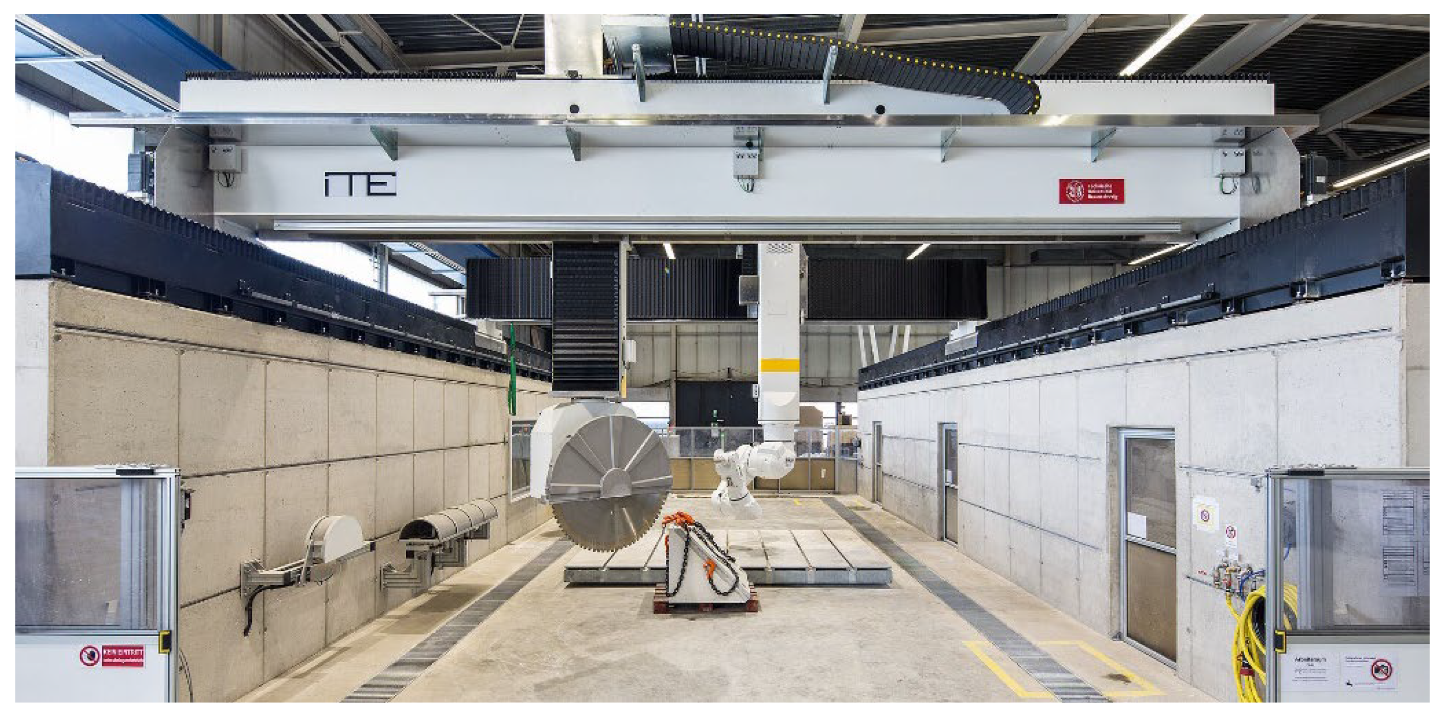
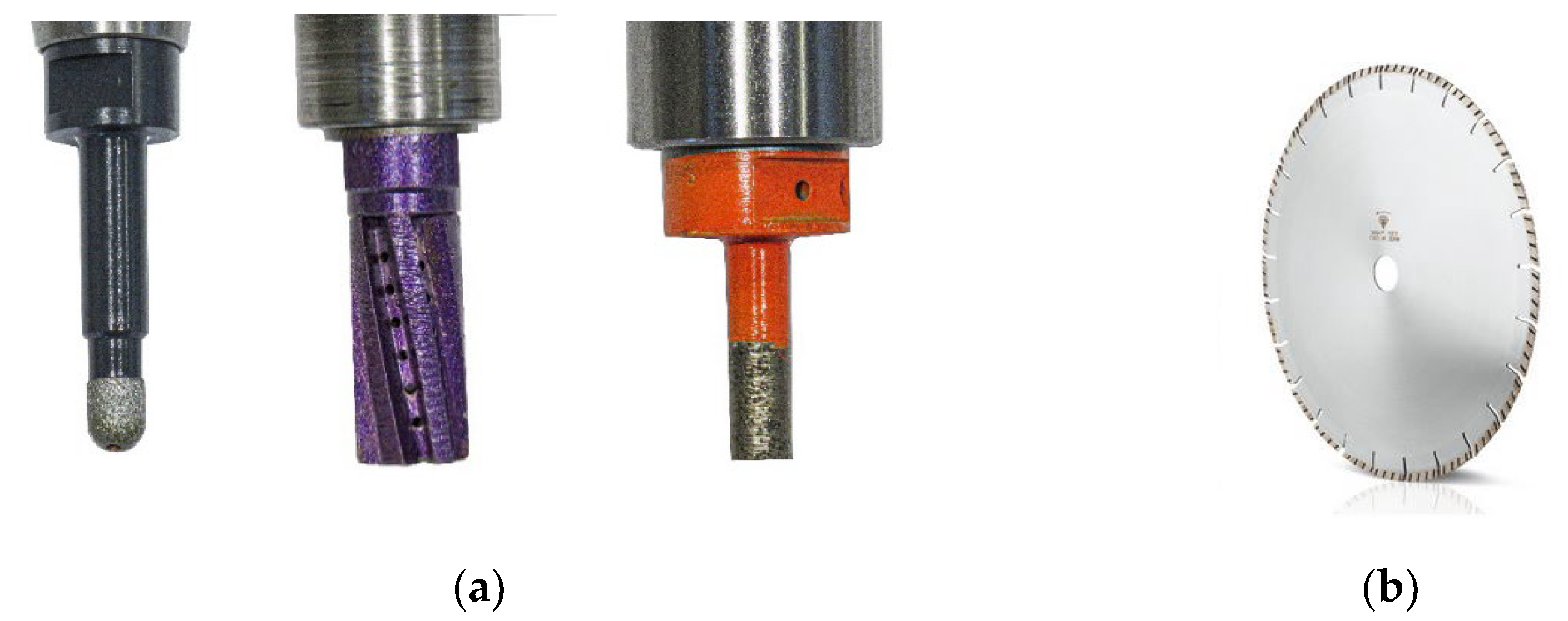
• Score 4: A CNC-controlled circular saw (Figure 1c) works like a water jet. However, the diameter of the saw blades limits the manufacturing of edges and details in the joint profiles that are still manufacturable by water jetting.

When it comes to an evaluation criterion with quantitative data, like duration of jointing or joint quality, either assumptions are made, or preliminary tests are carried out. Regarding e.g., the joint quality, the maximum and minimum quantity of damageable edges and their length are counted for the joints in the catalogue. The joint with the maximum amount got a score of zero, and the minimum got a score of four. Score one to three are evenly distributed in between. These assumptions are listed in Table 2 and described in the following sections for each evaluation criterion.

3.1.1. Manufacturability

The manufacturability indicates that a joint profile can be manufactured by different production techniques. The CNC-milling (CNC), direct printing (DP), formwork (FW), water jet (WJ) and circular sawing (CS) techniques are currently part of AMC. If a larger number of techniques can be used to manufacture the joint profile, the score will be higher, as it would mean more versatility of the production process. Using the same logic, if the joint cannot be manufactured by any technique, it has a score of zero, considering the difficulty encountered to reproduce the profile. Basically, the scoring system follows arithmetically the number of alternatives that can be used to manufacture a specific joint profile. Every joint profile that is manufacturable by CNC is also manufacturable by DP. It is listed as one technique for the scoring in manufacturability.

For a better understanding, e.g., as recognised from experiments made by the Division of Concrete Construction of TU Braunschweig, a triangular or smooth joint profile can be manufactured by every technique proposed, thus, both profiles get a score of four. On the other hand, a Lego joint profile might only be manufactured by two techniques, so it gets a score of two.

Table 3. Scoring in evaluation criteria “manufacturability”.

-	Score
Criteria
[-]	[-]	[-]	[-]	[-]	[-]
Manufacturability	No technique can be used	Only one technique can be used	Two techniques can be used	Three techniques can be used	All four techniques can be used

shows an illustration for the assumptions of the criteria “manufacturability”.

3.1.2. Connectivity in a Structure

The evaluation criterion “connectivity in a structure”, important in terms of the practical use of those connections in real scale for the construction site, concerns the axis and directions in which the joint can be fitted. Female and male parts of joints can be connected in either axial, lateral and/or radial directions. Axial jointing means that the female and male parts of a joint can only be matched together perpendicularly. Lateral means that the female part of a joint can be pushed over the male part horizontally. Radial means that one part of the joint can be rotated for, e.g., 90° and still connect ideally with the other. The idea of the criteria “connectivity in a structure” is shown in Figure 3, exemplary for a triangular (Figure 3a), truncated pyramid (Figure 3b) and smooth (Figure 3c) profile.

Considering the scoring parameter, it is important to highlight that it does not follow exactly the arithmetical number of possibilities, because there are three possible ways and a score that goes up to four. To solve that problem and make it a homogenous score of four for all criteria, it is defined that the axial connectivity gets a higher score than the radial and lateral ones. Components like columns and beams, which are the most common around, are usually connected axially on the construction site. This gives a better approach to the realistic condition. Therefore, the final score is calculated as a sum of the points given. To clarify the scoring system the following examples are presented and shown in

Table 4. Scoring in evaluation criteria “connectivity in a structure”.

-	Score
Criteria
[-]	[-]	[-]	[-]	[-]	[-]
Connectivity	Axial, lateral, radial	radial lateral	axial * lateral, radial	axial, radial axial, lateral	axial, lateral, radial
Calculation basis	No connectivity by any means	1	2 or 1 + 1	2 + 1	2 + 1 + 1

* Axial alone gets a score of two due to the most similarity with the real construction field.

:

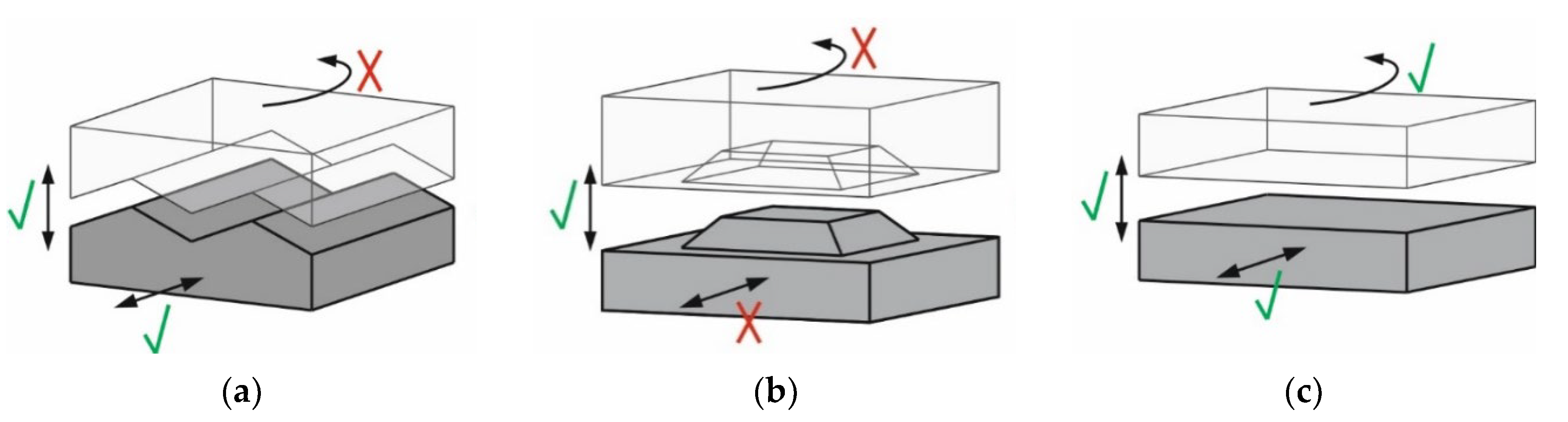
• A smooth joint profile can be jointed in every direction, axial, lateral and radial, which would give it the highest score, in this case a score of four, because it means that profile can be assembled easily compared to some others.
• A triangular joint can be assembled axially and laterally. Therefore, it gets a score of three, which equals to two (axial) plus one (lateral).
• A point shape joint profile might only be connected axially and radially. Therefore, it gets a score of three as well, which equals to two (axial) plus one (radial).

3.1.3. Detachability

The evaluation criteria “detachability” links to the criteria displaying “connectivity in a structure. Dry joints might mainly be detachable, but not in every direction. An interlocked joint like a saw tooth profile is detachable in lateral, but not axial or radial directions. A trapezoid joint profile is, e.g., detachable in lateral and axial directions, but not radially. A smooth joint might be detachable in axial, lateral and radial directions.

3.1.4. Duration of Manufacturing

The evaluation criteria “duration of manufacturing” describes the time required to manufacture a joint profile with the techniques mentioned in Section 3.1.1. As there are many post-processing techniques available, all joint productions are correlated to CNC-milling because most of the joint profiles can be manufactured by this technique. As the height of the milling is always set to 10 mm, the milling volume is not sufficient to evaluate the duration. For example, a fungal joint profile has the same milling volume as a triangular joint profile but a more complex geometry. Due to the complex geometry, the manufacturing duration is assumed to be higher than the simpler geometry. So instead of the milling volume, the joint’s surface area is considered to evaluate the duration of manufacturing. If the surface of a joint profile is, e.g., higher than 200 cm², the CNC-milling required a lot of time, and the joint gets a low score. The profile where the surface is between 100 and 120 cm² gets highest score.

Table 5. Scoring in evaluation criteria “duration of manufacturing”.

-	Score
Criteria
[-]	[cm2]	[cm2]	[cm2]	[cm2]	[cm2]
Duration of manufacturing	$O_{\mathrm{j}}\ge 200$	$200>O_{\mathrm{j}}\ge 160$	$160>O_{\mathrm{j}}\ge 140$	$140>O_{\mathrm{j}}\ge 120$	$120>O_{\mathrm{j}}\ge 100$

lists the ranges of the surface areas belonging to the scoring.

Besides the geometric approach for evaluating the manufacturing duration in Table 5, preliminary CNC-milling tests are supposed to confirm the assumptions. Therefore, rectangular concrete specimens were subtractive post-processed by CNC-milling. The smooth (Figure 4a), arc (Figure 4b), trapezoid (Figure 4c) and sinusoidal (Figure 4d) joint profiles were manufactured, and their durations of manufacturing were measured. Figure 4 shows the samples with the joint profiles, the duration of manufacturing and the calculated area of the surface.

The results of the duration measurement show that it correlates with the surface of the joint profile. Preparing a smooth joint with CNC-milling only took 18 min. A preparation with other subtractive post-processing, like a water jet or a circular saw, might be even faster. CNC-Milling of an arc, trapezoid or sinus wave joint configuration took quite a long time, respectively, 74, 97 and 106 min. Besides the area of the joint surface that correlates with the duration of manufacturing, trapezoid, arc, and sinus wave joint profile types also required more than one milling tool. The more complex the joint profile is, the more tools are required, and the duration of manufacturing rises.

3.1.5. Joint Quality

The evaluation criteria “joint quality” considers possible damages and inaccuracies of the joint profile. The damages and inaccuracies of a joint profile might be caused by the energy of the subtractive post-processing tool. Joint profiles with more edges and brittle configurations are more likely to show damage and inaccuracies, while the number of damages is also related to the milling directions (toward/outward) and the properties of the concrete material.

Besides, the complexity of the edges of the unit specimen may affect the potential for damage; a smooth joint profile shows, e.g., no additional edges that might be damaged. In contrast, a checkerboard profile shows many sharp edges that might be damaged by the subtractive post-processing tool. In addition, this geometry demands high accuracy to ease the fitting. Furthermore, as all CNC-tools operate with rotary engines, milling sharp edges in the case where the profile has low accessibility is remarkably difficult, e.g., for a rectangular female part of the checkerboard joint. It principally shows the preferences of adding fillet-curve to all the joint’s edges, which further helps in reducing the stress concentration for better load transition.

Additionally, the angles of the edges must be considered to evaluate the joint quality. The probability of getting damage on an edge with an angle higher than 135° (reflex angle) might be less than for an edge with an angle of 20°. For this reason, edges with an angle bigger than 135° are not considered for evaluation.

Table 6. Scoring in evaluation criteria “joint quality”.

-	Score
Criteria
[-]	[Num.]	[Num.]	[Num.]	[Num.]	[Num.]
Joint Quality	$N_{\mathrm{E}}>20$	$20\ge N_{\mathrm{E}}>15$	$15\ge N_{\mathrm{E}}>10$	$10\ge N_{\mathrm{E}}>5$	$5\ge N_{\mathrm{E}}$

lists the number of edges and their score in the evaluation criteria “joint quality”.

It must be highlighted that the joint quality should not be confused with the accuracy of the joint, i.e., how good the female and male parts of a joint fit each other. The evaluation of the accuracy of the joints is part of WP2 (Figure 2). After the subtractive post-processing, a laser scanned the joint profile, and the results are compared with the intended profile.

3.1.6. Tensile Strength

As long as no steel reinforcement is used in the dry joints, they should face no tensile stresses. However, it might be still possible that a post-tensioned joint gapes open in the ultimate limit state. Regarding this, the joint profiles in the catalogue should be evaluated by tensile stress transmission. If the joint is not interlocked, no tensile stresses might be transferred from the female to the male part of the dry joint. Therefore, an interlocking joint is required for evaluation. The evaluation of the tensile strength of a joint profile is done using the area of the interlocked joint that has to rupture if exposed to tensile loading. The higher that failure area is $\left(\sum l_{\mathrm{i},\mathrm{n}}\right)$, the higher is the score in the evaluation criteria. Figure 5 illustrates the assumption of the area that must fail in a dovetail (Figure 5a), knob (Figure 5b), and fungal (Figure 5c) joint profile. This type of strength generally demands the geometries that limit the fitting directions and have higher tangential friction during the assembly, which cause some difficulties in the fitting time and may lead to unwanted damage.

3.1.7. Shear Strength

A similar approach to the one described above is used for the evaluation of the shear strength. The joint is assumed to be tested under shear with no possibility of horizontal displacement, according to Figure 6. It is supposed that the load cannot separate the female and male parts and that the profile (resp. cams) must shear off. The imaginary sheared off area is summed up. Ideal material behaviour is also required for this assumption. The shearing area in the case of shear failure is determined by imagining a shear test. The shear area of an arc joint is half the size of the cross-section (see Figure 6a). A trapezoid joint’s shear area is less than the arc joint (see Figure 6b). This results in a better evaluation of the criteria “shear strength” and a higher scoring in the joint catalogue of the arc joint compared to the trapezoid joint. The highest shear area is in the triangular joint, with two-thirds of the total joint length. The assumption also requires a unit slope and number of teeth in a joint hence the joint comparison is possible among themselves. A line-shape joint shall always have two teeth, a point-shape joint has only one tooth, and a mesh-shape joint has at least four teeth.

3.1.8. Torsional Strength

The torsional strength is evaluated by the joint area that must shear off under torsional loading. A truncated cone has, e.g., no torsional strength, while a truncated pyramid joint shows high torsional resistance.

3.1.9. Failure Mode

The evaluation criterion “failure mode” grades the joints according to the stress-bearing behaviour in general. It is divided into compression, shear, tensile and torsional stresses, and linked to the other evaluation criteria. All joints are, e.g., able to resist against compressive loading and all line- and point-shaped joint profiles can transfer shear stresses. A smooth joint could, e.g., only bear compressive loading and a napped profile requires a post-tensioning to bear shear stresses. If a joint is, e.g., able to resist all stresses, it got the highest scoring of four. If it can not bear any stress, it gets no score.

3.1.10. Compression Strength

The compressions strength is evaluated in two ways: by a simple approach and FE analyses (see Section 4). The simple approach consideres inclined areas as “imperfections” in a joint. It is assumed that imperfections reduced the compression strength of a joint. Furthermore, the inclination area is multiplied by the angle of inclination because steeper inclined areas have a higher effect on compressive strength than flat surfaces. Figure 7 shows the approach to evaluate the compressive strength by a triangular joint (a), a saw tooth joint (b) and a trapezoid joint (c).

A triangular joint (Figure 7a) has, for example, four imperfection areas ①, ②, ③ and ④, while a saw tooth joint (Figure 7b) has only two imperfection areas ① and ②. One imperfection area of a saw tooth joint is approximately twice the size of an imperfection area of the triangular joint. That is why the inclination angle of the imperfection area must be considered. The inclination angle of an imperfection area in a triangular joint is approximately double of an imperfection area in a triangular joint. Summing up all imperfection areas $l_{\mathrm{i}}$ and multiplying them with the inclination angles ${\alpha }_{\mathrm{i}}$ results in a value $N_{\mathrm{Rd},\mathrm{tho}}$ that characterizes the compressive strength of a joint. The higher $N_{\mathrm{Rd},\mathrm{tho}}$ is, the less is the compressive strength and, therefore, the scoring of the evaluation criterion. Equation (1) shows the formula for the compressive strength evaluation. This measurement also has a direct relation with the ageing and cost of the milling tools.

$$N_{\mathrm{Rd},\mathrm{tho}} = {\displaystyle \sum }_{n = 1}^i{l}_{\mathrm{i}} · {\alpha }_{\mathrm{i}}$$

(1)

3.2. Weighting Factors

Besides scoring, the joint catalogue also contains weighting factors. Weighting factors shall regard the aims of the C05 subproject in TRR 277. The main goals of the C05 subproject are the comprehension of the load-bearing behaviour of dry joints under compression and shear as well as their FE analysis. The next important points are the manufacturability, connectivity and duration of manufacturing the joint profiles. Other important issues are the detachability of the joints, which shows its importance in recycling and reusing the concrete elements. Likewise, joint quality (not to be confounded with the accuracy of fit), torsional strength and failure mode are the highlighted additive criteria. Thus,

Table 7. Weighting factors of evaluation criteria.

Criteria	Weighting Factor
Manufacturability	2
Connectivity	2
Detachability	1
Duration	2
Joint quality	1
Tensile strength	1
Shear strength	3
Torsional strength	1
Compressive strength	3
Failure Mode	1
FE analysis	3

contains the weighting factors according to what suits best the priority of the evaluated criterion.

3.3. Algorithm

The algorithms should be kept easy in handling and calculation. The algorithm is a simple approach where the score $S_{\mathrm{i}}$ of the evaluation criteria is multiplied by the weighting factors $X_{\mathrm{i}}$ and sum up to the overall score $S_{\mathrm{EC}}$. Equation (2) shows the formula for the algorithm.

$$S_{\mathrm{EC}} = {\displaystyle \sum }_{n = 1}^i{X}_{\mathrm{i}} · S_{\mathrm{i}}$$

(2)

Furthermore, the algorithm gives the possibility of flagging. Flagging means that the joint will not be evaluated by any criteria. The flags are divided into two colours: green and red. A green flag leads to a direct selection of the flag for further numerical and experimental investigations. A red flag means that the joint profile is not suited for concrete constructions and will not be regarded for evaluation.

Table 8. Joint profiles with score of algorithm.

Joint Profile	Category	Drawing	Score
Triangular	Line-shaped		50
Saw tooth	Line-shaped		49
Sinusoidal	Line-shaped		47.5
Arc	Line-shaped		47.5
Trapezoid	Line-shaped		38.5
Dovetail	Line-shaped		28.5
Fungal	Line-shaped		29
Shell	Point-shaped		38.5
Inner Circle	Point-shaped		37.5
Cross	Point-shaped		37.5
Truncated cone	Pont-shaped		40.5
Truncated pyramid	Point-shaped		49.5
Smooth	Mesh-shaped		45
Chequerboard	Mesh-shaped		Red flag
Lego	Mesh-shaped		36
Fish-scale	Mesh-shaped		41

shows the joint profiles that have the highest overall score calculated by the algorithm.

Based on the results, AMC’s best joint profile is the triangular profile with an overall score of 50 out of 68 possible points. It has a desirable behaviour in shear and is easy to produce. The saw-tooth, sinus wave, arc and truncated pyramid profiles also have a noticeably high overall score and are well suited for AMC structures. It is remarkable that the trapezoid joint, which is already established in the segmental building industry, has only a score of 38.5. The reason might be the different perspective of the conventional building industry compared to the digital building industry, like AMC. In AMC, other criteria, like the joint quality or the duration of manufacturing, for choosing a joint profile are more important compared to in the conventional building industry.

Dovetail and fungal joints are rated as the most inappropriate connection types. The main disadvantage of these joints is the elaborate manufacturing necessary in the case of concave surfaces. Another point against the dovetail and fungal joints is the connectivity in the entire structure because they can only be fitted in one direction. However, they are joints that can transfer tensile forces. However, transferring tensile stresses in unreinforced concrete structures is generally risky due to brittle material behaviour.

4. Preliminary Finite-Element-Analysis

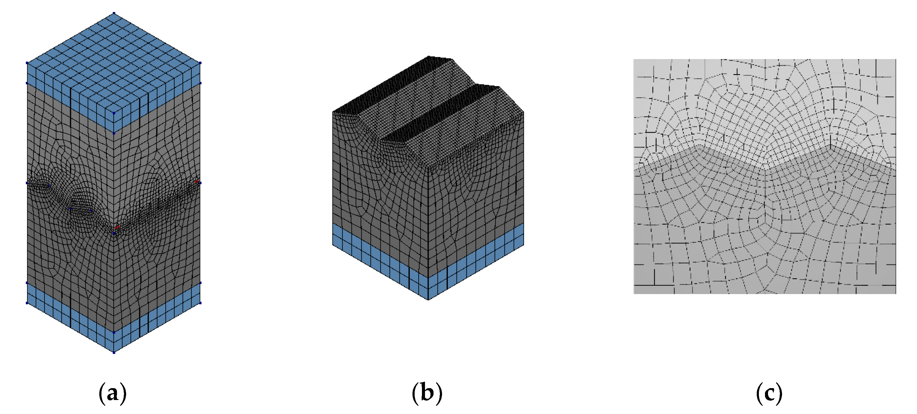
4.1. Geometric Model

All FE analyses are conducted with the software DIANA FEA [29]. The geometries of the jointed specimens are idealized as isoparametric solid elements with two steel plates on the upper and bottom parts for uniform load distribution. The model’s dimensions are adapted to the planned test set-up of work package WP2, showing a 100/100 mm cross-section and a height of 200 mm in total. The joint profiles are located between both solids, connected by an interface element. The steel plates are linked to the end faces of the specimens monolithically to ensure an even load transmission, simulating the test set-up as planned in the experimental investigations. Figure 8 shows the geometric model of the preliminary FE analysis.

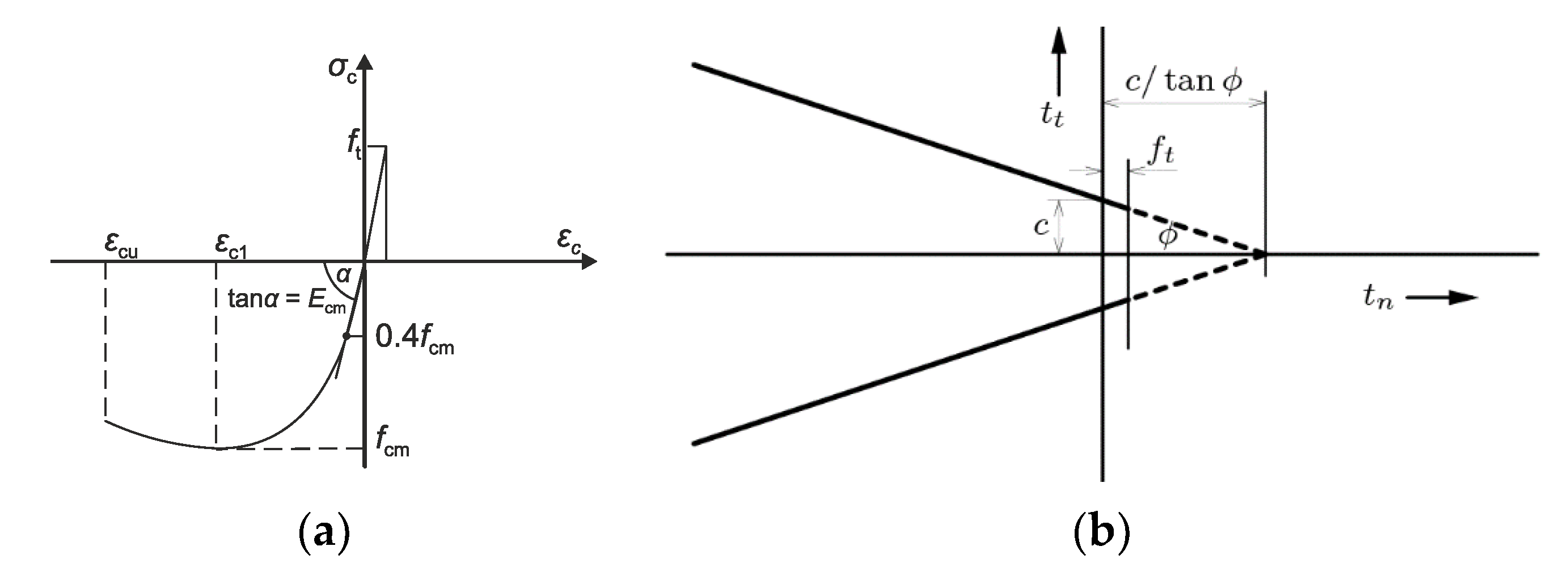
4.2. Material Models and Properties

The steel plates are regarded considering a linear-elastic stress-strain relationship with a Young’s modulus of 200.000 MPa. The concrete is modelled with a non-linear material model to detect failure. Therefore, the “total strain-based crack model” (TSBCM) is used [29]. The TSBCM is based on an approach from the Model-Code 2010 [30] for compression, and it uses a brittle stress-strain relationship for tensile behaviour. Figure 9a shows the material models for compression and tensile behaviour. As the FE analyses are preliminary, the material “tailored” properties of 3D-printed concrete are not considered.

The joint between the concrete elements is modelled as an interface with linear elasticity and Coulomb Friction [7]. As the material parameters of the concrete model are set as fixed, the input values for the interface model need a modification for dry joints. Figure 9b shows the Mohr Coulomb friction model.

Assuming that dry joints have no cohesion, parameter c equals zero. The friction coefficient of concrete is approximately $\mu = \left[0.60–0.70\right]$ according to the literature [31] and assumes a smooth surface texture. The friction coefficient will be measured precisely in the experimental investigations depending on the subtractive post-processing (CNC, circular saw) and adapted later. However, for the first evaluations, it is set to $\mu = 0.70$. Furthermore, it is assumed that the dilatancy angle of the Coulomb Friction Model equals the angle of friction with $\psi = \mu = 0.70$, according to [32].

The interface model also requires stiffness-moduli in perpendicular (normal) and horizontal (shear) directions. For a rigid connection, used in the vertical direction, the normal-stiffness-modulus is set to a value, which is higher than the concrete Young’s modulus. For the shear-stiffness-modulus, the value selected is much smaller than in the vertical direction to represent a hinge.

Table 9. Input values for interface model.

Model Parameter	Unit
[-]	[-]
Cohesion	$c=0.0$
Friction Coefficient	$\mu =\tan \phi \approx 0.70$
Dilatancy angle	$\psi =\phi \approx 35.0°$
Normal stiffness	50,000 N/mm3
Shear stiffness	100 N/mm3

lists the input values of the interface model.

4.3. Boundary Conditions

For the numerical analysis, boundary conditions must be first defined to apply general equations for the specific problem. In this case, it is favourable to describe the load as a displacement because of the possible integration of the equation system, reducing the calculation time. Next, following the convergence criteria, it is necessary to set two supports at the bottom of the system, preventing vertical and horizontal displacements, in the same manner as it is in the experimental setup. Therefore, the supports are set as tied to the steel plate underneath the concrete and placed in one corner. A single load is also placed in a corner and related to the whole surface by tying. The value for the displacement amounted to 0.1 mm and the load simulated the force from the experiment.

4.4. Mesh Properties

The element sizes in the mesh varies in the longitudinal direction (Figure 10a,b). Near the load transmission plates, the element size is equal to 10.0 mm, but near the joint to 2.0 mm (Figure 10c). Thereby, the concrete element is divided into 10 pieces in the general area and into 50 pieces around the joint. Figure 10 shows the model used, and the variable mesh size chosen for the simulation. By using these dimensions, an acceptable optimal condition is found, considering convergence, accuracy, and least calculation effort.

4.5. Analysis

As a material model that included the concrete damage is used, 50 load steps described the load. Therefore, each load step consists of 0.002 mm displacement. As previously mentioned, the convergence of the system is ensured by the resulting force and energy, as displacement is described as the load. Furthermore, the linear-stiffness method is selected as the solution method. This solution algorithm solves non-linear equations by building the stiffness matrix only once and doing the iterations by determination of the imbalance load. The iterations stops when the system either passes predefined convergence criteria or by reaching a maximum number of iterations. In the view of convergence, some may argue that this method is the slowest [29]. However, due to the used material model, there is no significant non-linearity expected. Therefore, the linear-stiffness method still appears as the best option, having a time-advantage for each iteration, reducing the overall considered calculation time.

4.6. Simulation Results

The objectives of the numerical investigations are to examine the normal load-bearing capacity of the joint configuration and to understand the stress distribution in the direct vicinity of the joint profile.

Table 10. Load-bearing capacity within the FE analysis regarding different joint profiles.

Joint Profile	Ultimate Load	Joint Profile Factor
[-]	[kN]	[-]
Monolithic	$396$	1.0
Smooth	396	1.0
Triangular	361	0.91
Saw tooth	387	0.97
Sinusoidal	365	0.92
Arc	389	0.98
Truncated Pyramid	380	0.96

lists the ultimate normal loads $F_{\mathrm{u}}$ of the simulated tests regarding the different joint profiles as well as a joint profile factor $\left(F_{u,segmental}/F_{u, monolithic}\right)$.

The so-called joint profile factor shows that the ultimate normal load of the jointed specimens is always more than 90% of the reference load of the monolithic specimen. The smooth joint shows the highest load-bearing behaviour, being the same as for the monolithic specimen. The most suitable joint profile for normal load transfer in compression is the arc configuration with a joint profile factor of 0.98. The preliminary results of the FE analysis confirm the assumptions made in the theoretical investigations of the joint catalogue.

5. Joint Selection

The results of the evaluation process in the joint catalogue and the preliminary FE analysis showe that the smooth, triangular, saw-tooth, sinusoidal, arc, and truncated pyramid best suit dry joints in AMC. The smooth, triangular, arc and truncated pyramid joint profiles are, therefore, selected for further experimental and numerical investigation (Figure 11).

6. Preparation for Joint Production

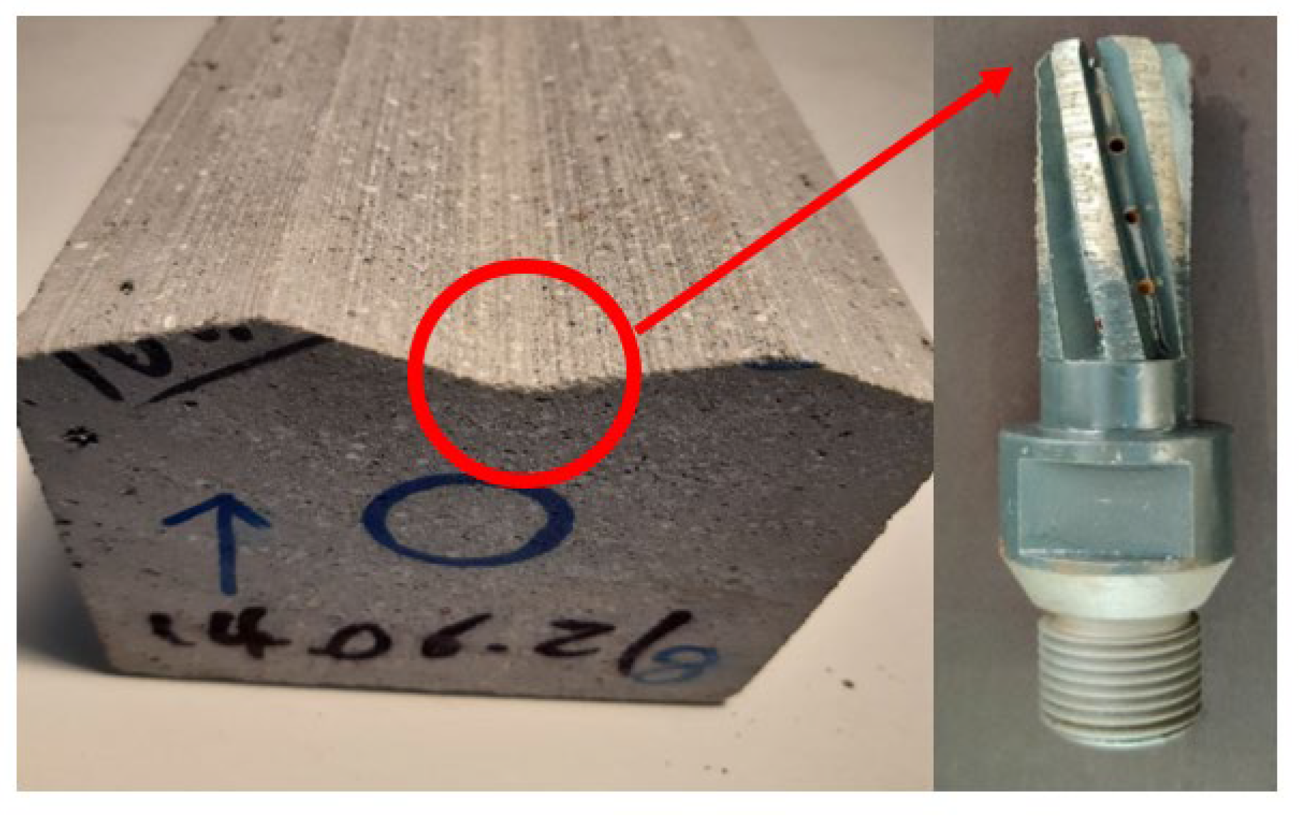
6.1. Subtractive Post-Processing

Robotic subtractive processing, as the robotic concrete printing’s complementary technique, has proved its potential; hence as initially noticed, fundamentally discussing the geometries of dry concrete connections is becoming an important issue that needs to be scientifically addressed. The current TRR277 subproject (C05), through all work packages (WP1–WP4), operates the CNC-process in the Digital Building Fabrication Laboratory (DBFL), see Figure 12.

The DBFL laboratory is unique in its conception and execution. The DBFL contains two main portals: the robotic arm with 12 axes, e.g., utilized for 3D concrete printing, and the second portal, with nine axes, e.g., as used in C05 for concrete CNC. In the initial Section 2 and Section 3.1, the superiority of the CNC-milling was discussed in comparison to other methods (e.g., casting and waterjet). Nonetheless, this method also has limitations in manufacturing different geometries. The limitation has two main reasons.

• Utilization of the rotary CNC-engines leading to typical rotating milling/sawing tools, which are only suitable for round geometries.
• Low accessibility of the CNC-arm to different sides of the geometry. Several simple joint geometries need the rotating milling tools to approach from different sides, which may easily cause a collision between the tools and the concrete specimens or the rotary engine and the clamping table.

The initial CNC-simulations can measure these difficulties and most of the criteria mentioned in the catalogue. The CNC-simulation is mainly essential for producing the G-codes to be sent to DBFL’s central computers. The G-codes are made by EasyStone [33] (CNC-software) in these work packages. EasyStone, in addition to the dimensions and permanent details of DBFL’s features, includes the type and dimensions of the available milling/sawing tools in the tool magazine that are to be applied in the G-codes and can change the tool during the CNC-process. In addition to preparing the G-codes, these simulations can be used to score some of the catalogue’s criteria, mainly related to the manufacturing difficulties such as estimating the milling duration, etc.

The CNC-technique has been utilized for around two centuries; nonetheless, robotic manufacturing dry concrete connections is a new developing technique, and the challenges before the industrial usages should be faced. The main challenges, in addition to the limited producible geometries, are:

• High duration of the CNC-process;
• Dependency on the dissimilar properties of concrete, which may easily cause unwanted damage due to the low quality and high brittleness of this material;
• Fast ageing or abrasion of the milling tools, which in addition to increasing the CNC-costs, influences the accuracy of the geometries and difficulties in the fitting.

6.2. CNC-Tools

A wide range of milling tools can manufacture dry concrete joints. The tools can be classified regarding the size type etc. For instance, as a classification in WP1–WP3, three types of tools, including saw blades, rough milling tools (different sizes) and finishing milling tools (different sizes and shapes), are used (see Figure 13).

These are standard CNC-tools, while—in the case of frequent CNC-milling or -sawing of one recurring type of geometry—customized tools can improve the accuracy and accelerate the process but reduce the limitation in the manufacturable geometries. This means, the geometry of the milling tool equals the geometry of the joint profile. For example, in milling the wave shape (sinusoidal) geometry, instead of time-consuming milling, a customized milling tool with exact parallel geometry of parallel waves can be selected. Otherwise, a time-consuming process with two rough and finishing steps with several parallel milling movements is needed with gradually degree changes for the curves. Likewise, some geometries essentially need special milling tools. For instance, the female parts of the mentioned checkerboard connection, due to limited access and the round shape of the milling tools, cannot be produced by standard milling tools. This manufacturing needs special tools, like square CNC (e.g., milling mortise chisel) to be customized for concrete.

6.3. Abrasion of Milling Tools

One main difficulty of the CNC-tools is the noticed ageing (abrasion) of them, which directly affects the costs and accuracy of the process (see Figure 14). The ageing problem becomes challenging, while the ageing speed or the abrasion (percentages) does not have a known, gradual process or rate, but instead, is dependent on several parameters, including the type of joint’s geometries, the milling side of the tool, milling speed and quality of the concrete. This issue can be mitigated by frequently changing the tools, successive calibration of the milling tool or scanning the joint geometry for measuring the influence of the tool’s abrasion on the final geometry.

6.4. Accuracy of Milling

In addition to tools ageing, the geometrical accuracy of the joints is influenced by several other points, such as: the prepared G-codes, precision of the milling tools’ calibration, the type of the selected milling tools, the complexity of the joint’s geometries, the selected milling clamping tools, the milling speed and the properties of the concrete. To evaluate the accuracy of the manufactured joint, the micro-scans of several DBFL-milled dry connections were compared to the CAD models, focusing on the jointing profiles or surfaces. The maximum geometrical errors, considering differences between the profiles of milled joints and CAD files of the joint, was one of the calculated criteria. The range of absolute maximum geometrical errors regarding 100 comparing areas was [0.03833 mm, 0.8453 mm].

Generally, especially in complex connections with high fitting friction, negative scale (error) might be essential for practical fitting the geometries. Nonetheless, geometrical errors in negative and positive amounts can cause issues. Issues in negative error cause a gap between the joints, and positive error brings difficulties in the fitting. These might cause some difficulties, including probable stress concentration, asymmetric performance, changing the failure mode, local failure, and movement, which may reduce the effect of post-tensioning loads, etc.

7. Conclusions and Outlook

The investigations presented in this paper were carried out within the framework of the TRR 277 subproject C05. Many different joint profiles were collected in a joint catalogue. Various criteria evaluated the processing and the performance of these profiles. Based on the assessment of the joint profile in the evaluation criteria, every joint profile gets a score. The score is multiplied by a weighting factor and summed up to an overall score. The joint profiles with the highest score were selected for further numerical and experimental investigations.

• Thirty-one joint profile configurations were gathered in a catalogue and categorized as line-shaped, point-shaped or mesh-shaped.
• The joint profiles were evaluated by various criteria like manufacturability, connectivity in a structure, detachability, duration of manufacturing and stress transfer.
• The evaluation criteria were mostly based on geometric approaches, e.g., the milling surface of the joint profile correlates with the duration of manufacturing the joint profile.
• An algorithm multiplied the score of each evaluation criterion with a weighting factor and sums up the scores to an overall score.
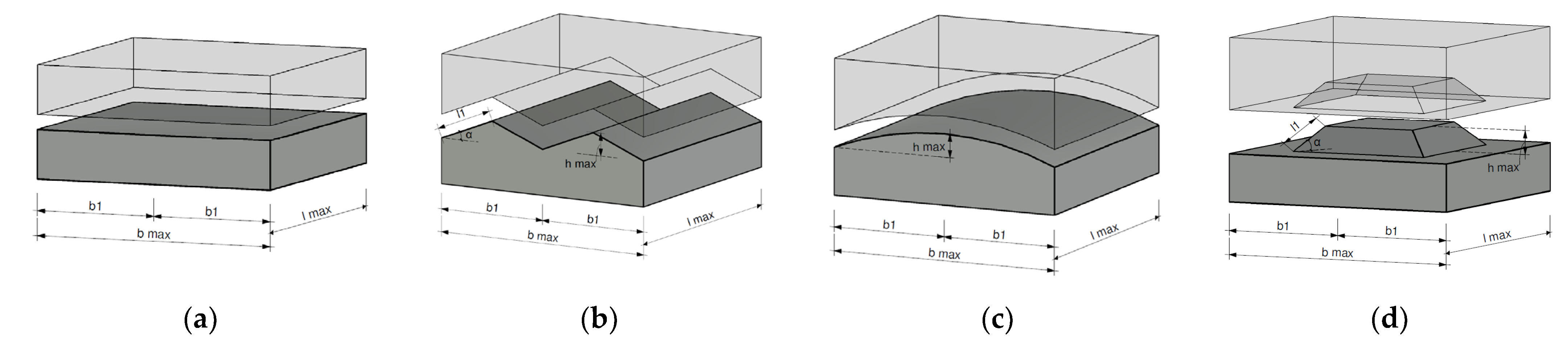
• The preliminary FE analysis showed that a smooth, arc and saw tooth joint profile performed more desirably under normal compression loading.
• The algorithm selected smooth, triangular, arc and truncated pyramid-joint profiles in the joint catalogue for further numerical and experimental investigations.

In the next step, the specimens with the selected joint profiles will be manufactured by using all existing additive manufacturing techniques (extrusion, shotcrete, and particle-bed). At this, the joint profile geometry will be CNC-milled or CNC-sawed into the specimen. Experimental testing under compression and shear will then give further knowledge about the load-bearing behaviour of dry joints in 3D-printed concrete elements.

References

1. Kloft, H.; Gehlen, C.; Dörfler, K.; Hack, N.; Henke, K.; Lowke, D.; Mainka, J.; Raatz, A. TRR 277: Additive Fertigung im Bauwesen [TRR 277: Additive Manufacturing in Construction]. Bautechnik 2021, 98, 222–231. [Google Scholar] [CrossRef]
2. Dielemans, G.; Dörfler, K. Mobile Additive Manufacturing: A robotic system for cooperative on-site construction. In Proceedings of the International Conference of Intelligent Robots and Systems (IROS), Workshop Robotic Fabrication: Sensing in Additive Construction, Prague, Czech Republic, 27 September–1 October 2021. [Google Scholar]
3. Lindemann, H.; Gerbers, R.; Ibrahim, S.; Dietrich, F.; Hermann, E.; Dröder, K.; Raatz, A.; Kloft, H. Development of a Shotcrete 3D-Printing (SC3DP) Technology for Additive Manufacturing of Reinforced Freeform Concrete Structures. In First RILEM International Conference on Concrete and Digital Fabrication—Digital Concrete; Springer: Berlin, Germany, 2018; pp. 287–298. [Google Scholar]
4. Maboudi, M.; Gerke, M.; Hack, N.; Brohmann, L.; Schwerdtner, P.; Placzek, G. Current Surveying Methods for the Integration of Additive Manufacturing in the Construction Process. In The International Archives of the Photogrammetry, Remote Sensing and Spatial Information Sciences:XXIV ISPRS Congress Volume XLIII-B4-2020; Copernicus Publications: Gottingen, Germany, 2020. [Google Scholar]
5. Xiao, J.; Ji, G.; Zhang, Y.; Ma, G.; Mechtcherine, V.; Pan, J.; Wang, L.; Ding, T.; Duan, Z.; Du, S. Large-scale 3D printing concrete technology: Current status and future opportunities. Cem. Concr. Compos. 2021, 122, 104115. [Google Scholar] [CrossRef]
6. Xiao, J. 3D recycled mortar printing: System development, process design, material properties and on-site printing. J. Build. Eng. 2020, 32, 101779. [Google Scholar] [CrossRef]
7. Wichert, M.; Matz, H.; Empelmann, M. Grouted Segment Joints for Structures Made of Ultra-High Performance Concrete. In Proceedings of the Fib Symposium 2019, Krakow, Poland, 25–27 May 2019; Derkowski, W., Gwoździewicz, P., Hojdys, L., Krajewski, P., Pańtak, M., Eds.; pp. 2231–2238. [Google Scholar]
8. Oettel, V.; Empelmann, M. Load-Bearing Capacity of Profiled Dry Joints between Adjacent UHPFRC Precast Elements. In Proceedings of the Fib Congress 2018, Melbourne, Australia, 7–11 October 2018; Foster, S., Ed.; pp. 344–345. [Google Scholar]
9. Robert-Wollmann, C.L.; Breen, J.E.; Kreger, M.E. Temperature Induced Deformations in Match Cast Segments. PCI J. 1995, 4, 62–71. [Google Scholar] [CrossRef]
10. Full-Scale 3D Printed Concrete Bicycle Bridge Destined for Gemert. Available online: http://www.3ders.org/articles/20170907-massive-3d-printed-bicycle-bridge-is-delivered-to-gemertnetherlands-by-truck.html (accessed on 27 March 2018).
11. Reichel, M. Dünnwandige Segmentfertigteilbauweisen im Brückenbau aus gefasertem Ultrahochleistungsbeton (UHFB) [Thin-walled Precast Segmental Bridge Structures Made of Fiber-Reinforced Ultra-High Performance Concrete (UHPFRC)]. Ph.D. Thesis, TU Graz, Graz, Austria, 5 December 2010. [Google Scholar]
12. Oesterle, S.; Vansteenkiste, A.; Mirjan, A. Zero Waste Free-Form Formwork. In Proceedings of the Second International Conference on Flexible Formwork, Bath, UK, 27–29 June 2021; BRE CICM, University of Bath: Bath, UK, 2012. [Google Scholar]
13. Hyun-O, J.; Han-Seung, L.; Keunhee, C.; Jinkyu, K. Experimental study on shear performance of plain construction joints integrated with ultra-high performance concrete (UHPC). Constr. Build. Mater. 2017, 152, 16–23. [Google Scholar]
14. Knitl, J. Hybrid towers for wind power plants in precast construction—Efficient electric power generation. BFT Int. 2014, 2, 54–55. [Google Scholar]
15. Lachmayer, L.; Ekanayaka, V.; Hürkamp, A.; Raatz, A. Approach to an optimized printing path for additive manufacturing in construction utilizing FEM modeling. Procedia CIRP 2021, 104, 600–605. [Google Scholar] [CrossRef]
16. Reichel, M.; Sparowitz, L.; Freytag, B. Bridge WILD Völkermarkt—Prestressed arched structure made of precast UHPC-segments. Beton-Und Stahlbetonbau 2011, 106, 827–835. [Google Scholar] [CrossRef]
17. Reichel, M.; Altersberger, G.; Sparowitz, L. UHPFRC Prototype for a Flexible Modular Temporary High-speed Railway Bridge. In Designing and Building with UHPFRC: State-of-the-Art and Development; Resplendino, J., Toulemonde, F., Eds.; John Wiley & Sons: London, UK, 2011; pp. 263–277. [Google Scholar]
18. Gaston, J.; Kriz, L. Connections in Precast Concrete Structures—Scarf Joints. PCI J. 1964, 10, 37–59. [Google Scholar] [CrossRef]
19. Buyukozturk, O.; Bakhoum, M.; Beattie, S. Shear Behaviour of Joints in Precast Concrete Segmental Bridges. J. Struct. Eng. 1990, 119, 3380–3401. [Google Scholar] [CrossRef]
20. Kordina, K.; Teutsch, M.; Weber, V. Spannbetonbauteile in Segmentbauart; German Comittee for Reinforced Concrete (DAfStb): Berlin, Germany, 1984; p. 350. [Google Scholar]
21. Falkner, H.; Teutsch, M.; Huang, Z. Segmentbalken mit Vorspannung ohne Verbund unter kombinierter Beanspruchung aus Torsion, Biegung und Querkraft; German Comittee for Reinforced Concrete (DAfStb): Berlin, Germany, 1997; p. 472. [Google Scholar]
22. Specker, A. Der Einfluss der Fugen auf die Querkraft- und Torsionstragfähigkeit extern vorgespannter Segmentbrücken [The Influence of Joints on the Shear Force and Torsion Bearing Capacity of Externally Prestressed Segmental Bridges]. Ph.D. Thesis, TU Hamburg-Harburg, Hamburg, Germany, 2001. [Google Scholar]
23. Baghdadi, A.; Meshkini, A.; Kloft, H. Parametric design of in-plane concrete dry joints by FE method and Fuzzy logic toward utilizing additive manufacturing technique. In Proceedings of the IASS Annual Symposium 2020/21 and the 7th International Conference on Spatial Structures Inspiring the Next Generation, Guilford, UK, 23–27 August 2020. [Google Scholar]
24. Voo, Y.L.; Foster, S.J.; Voo, C.C. Ultra high-Performance Concrete Segmental Bridge Technology: Toward Sustainable Bridge Construction. J. Bridge Eng. 2015, 20, 16–23. [Google Scholar] [CrossRef]
25. Plank, M.; Reineck, K.-H.; Sobek, W. Dry Joints between Precast Elements made of UHPFRC. In Proceedings of the HiPerMat 2016 4th International Symposium on Ultra-High Performance Concrete (HiPerMat), Kassel, Germany, 9–11 March 2016; Fehling, E., Middendorf, B., Thiemicke, J., Eds.; Kassel University Press: Kassel, Germany, 2016. [Google Scholar]
26. Shin, J. Ultra-High Performance Concrete (UHPC) Precast Segmental Bridges. Ph.D. Thesis, TU Hamburg-Harburg, Hamburg, Germany, 2016. [Google Scholar]
27. Lehmberg, S.; Ledderose, L.; Mainka, K.H. Non-Standard joints for light-weight modular spatial and shell structures made from UHPFRC. In Proceedings of the IASS Annual Symposia; International Association for Shell and Spatial Structures (IASS): Madrid, Spain, 2014; Volume 2014, p. 11. [Google Scholar]
28. Baghdadi, A.; Heristchian, M.; Ledderose, L.K. Experimental and numerical assessment of new precast concrete connections under bending loads. Eng. Struct. 2020, 212, 110456. [Google Scholar] [CrossRef]
29. Manie, J. DIANA FEA—User’s Manual, Release 10.2. Available online: https://dianafea.com/manuals/d102/Diana.html (accessed on 1 July 2021).
30. FIB—Fédération Internationale du Béton. Fib Model Code for Concrete Structures 2010; Ernst & Sohn: Berlin, Germany, 2013. [Google Scholar]
31. Maissen, A. Festkörperreibung: Reibzahlen verschiedener Werkstoffe [Solid state friction: Coefficients of friction of different materials]. Schweiz. Ing. Und Archit. 1993, 111, 25–29. [Google Scholar]
32. Kueres, D.; Stark, A.; Herbrand, M.; Claßen, M. Finite element simulation of concrete with a plastic damage model—Basic studies on normal strength concrete and UHPC. Bauingenieur 2015, 90, 252–264. [Google Scholar] [CrossRef]
33. DDX Software Solutions S.r.l. EasySTONE “EasySTONE Manual”, version 4.9; Brembate di Sopra: Bergamo, Italy, 2013. [Google Scholar]
Figure 1. Subtractive post-processing of 3D-printed concrete: (a) nine-axle robot (b) fresh and (c) hardened concrete.
Applsci 12 04138 g001
Figure 2. Outline of C05 subproject in TRR277.
Applsci 12 04138 g002
Figure 3. Principles for jointing evaluation “connectivity in a structure”: (a) triangular (b) truncated pyramid and (c) smooth.
Applsci 12 04138 g003
Figure 4. Profiles for preliminary tests to measure the milling duration: (a) smooth (b) arc (c) trapezoid (d) sinusoidal.
Applsci 12 04138 g004
Figure 5. Principles for jointing evaluation “tensile strength”: (a) dovetail (b) knob (c) fungal.
Applsci 12 04138 g005
Figure 6. Principles for jointing evaluation “shear strength”: (a) arc (b) trapezoid (c) triangular.
Applsci 12 04138 g006
Figure 7. Exemplary evaluation of the compressive strength: (a) triangular (b) saw tooth and (c) trapezoid joint.
Applsci 12 04138 g007
Figure 8. The geometric model for FE analysis: (a) full FE model (b) half FE model and (c) interface connection.
Applsci 12 04138 g008
Figure 9. Material model for concrete: (a) Compression and tensile behaviour and (b) Mohr Coulomb friction model.
Applsci 12 04138 g009
Figure 10. Discretization of FE model: (a) Triangular model (b) half triangular model and (c) joint.
Applsci 12 04138 g010
Figure 11. Selected joint profiles for further investigations: (a) smooth (b) triangular (c) arc (d) truncated pyramid.
Applsci 12 04138 g011
Figure 12. Digital Building Fabrication Laboratory (DBFP).
Applsci 12 04138 g012
Figure 13. Different tools for subtractive post-processing: (a) milling tools and (b) saw blade.
Applsci 12 04138 g013
Figure 14. Abrasion of milling tools influences the joint profile accuracy.
Applsci 12 04138 g014