Article

Compressed Sensing Super-Resolution Method for Improving the Accuracy of Infrared Diagnosis of Power Equipment

School of Electrical & Electronic Engineering, North China Electric Power University, Baoding 071003, China
*
Author to whom correspondence should be addressed.
Appl. Sci. 2022, 12(8), 4046; https://doi.org/10.3390/app12084046
Submission received: 3 March 2022 / Revised: 11 April 2022 / Accepted: 12 April 2022 / Published: 16 April 2022
(This article belongs to the Topic Innovative Techniques for Smart Grids)

Abstract

:
The infrared image of power equipment plays a crucial role in identifying faults, monitoring equipment condition, and so on. The low resolution and low definition of infrared images in applications contribute to the low accuracy of infrared diagnosis. A super-resolution reconstruction method of infrared image, based on compressed sensing theory, is proposed. Firstly, by analyzing the variation of high-frequency information in infrared images with different blurring degrees, the image gradient norm ratio is introduced to estimate the blur kernel matrix in the degradation model a priori. Then, in the process of image reconstruction, we add the full variational regularization term to the traditional compressed sensing model, and design a two-step full variational sparse reconstruction algorithm. Experimental results verify the effectiveness of the method. Compared with the existing classical super-resolution methods, this method offers improvement in subjective visual effect and objective evaluation index. In addition, the final image recognition and infrared diagnosis experiments show that this method is helpful to improve the accuracy of infrared diagnosis of power equipment.

1. Introduction

With the proposal of the concept of the Internet of Things and the continuous promotion of the construction of the smart grid, the use of infrared diagnosis technology for real-time monitoring and fault diagnosis of power equipment can effectively improve the operation reliability of the power grid [1,2,3]. However, there is a wide range of electrical equipment in the power grid, and the large-scale deployment of expensive traditional high-resolution infrared sensors will cause enterprises to incur unbearable costs [4,5]. Therefore, how to use low-cost, low-resolution infrared sensors to achieve the effect of high-resolution infrared sensors is the key to promote the application of infrared diagnosis technology in the Internet of Things power system [6].
The main purpose of super resolution (SR) imaging technology is to overcome the limitations of low-cost and low-precision image acquisition devices. Through single- frame or multi-frame low resolution (LR) image input, it is necessary to complete image reconstruction according to different prior knowledge, obtain high resolution (HR) images, and recover high-frequency information lost in the process of image acquisition [7]. According to the number of LR images inputted during reconstruction, super-resolution can be divided into single-frame and multi-frame image super-resolution. Among these, multi-frame image super-resolution methods include the interpolation method [8,9], iterative back projection method [10], maximum likelihood estimation method [11], sparse coding method [12] and learning-based method [13,14]. The super-resolution method of multiple images uses complementary information contained in different images to improve the resolution by registering multiple images obtained at similar time positions in the same scene. The single-frame super-resolution method only uses a single image in a scene, which is more difficult. For the specific objective of infrared imaging of electrical equipment, the focus of super-resolution image reconstruction is not only clear structure and easy recognition, but also accurate response to equipment temperature. Multi-image super-resolution can easily cause the reflection of the reconstructed image to the temperature to lose accuracy, because the input low-resolution infrared images do not strictly come at the same time. This problem is particularly serious in the case of rapid change in equipment temperature, which is more concerning in the power industry. Therefore, the super-resolution method based on a single image can ensure accuracy of reconstruction.
The super-resolution methods based on a single image are mainly divided into three categories: interpolation-based, reconstruction-based and learning-based super-resolution methods. Among them, the super-resolution method based on interpolation is the simplest, but due to its inherent smoothing benefits, it is easy to lose details and blur the edges of the reconstructed image. Researchers have put forward various improvement measures for this problem [15,16,17]. The super-resolution method based on reconstruction [11,18,19] completes the inverse iterative solution, based on the image degradation model, by introducing a priori knowledge as the limiting condition. Reference [18] proposed a super-resolution algorithm based on nonlocal information. Shao et al. [19] calculated the blur kernel and high-resolution image at the same time. In the process of alternating iteration, a normalized sparsity measure is adopted, which is a generalized integral of relative total variation. It is used to represent the heavy tailed a priori characteristics of the image. For the accurate processing of a local image, Li et al. [11] adopted local structure self-similarity in the natural image to put forward the notion of turning kernel regression total variational, which is supplemented by the non-local total variational regular term to complete the establishment of the SR model. The main goal of the learning-based method is to find the corresponding relationship between HR image and LR image, usually by training an isomorphic dictionary or establishing both mapping relationships [20]. Kim et al. [21] proposed a low complexity adaptive single image super-resolution method. This method analyzes the input image and the corresponding low-resolution image to determine the intensity of the high-frequency component, while establishing the relationship between them. The effective addition of high-frequency information and high-quality image reconstruction are realized. Wang et al. [22] proposed the SFT-GAN model, which takes the image segmentation mask as the prior knowledge of single image super-resolutions to guide the texture reconstruction of different regions in single-image super-resolutions. Literature [23] offers a kind of latest method. It uses reinforcement learning to find the optimal network, which can reduce the influence of the manual on model design. This kind of method first defines a search space, uses the corresponding controller to process the search, outputs the reconstruction results after evaluation, and automatically adjusts them through network training until the network converges to get good reconstruction results.
The learning-based super-resolution method requires a large number of high-resolution infrared image samples. In super-resolution, the up-sampling rate is limited by the constructed model or isomorphic dictionary. The flexibility of the algorithm is low. In addition, the current super-resolution methods pay more attention to the accurate estimation of image degradation process. Efrat et al. [24] pointed out that in the super-resolution problem, the accurate estimation of the blur kernel representing the degradation process has a greater impact than the selection of the model. Therefore, in order to reconstruct infrared images with higher quality and accuracy, before establishing an accurate reconstruction model, we need to estimate the blur kernel.
Aiming at the problem of low resolution of infrared images obtained by infrared sensors of power equipment, this paper adopts the method based on reconstruction under the framework of compressed sensing. We analyze the change law of high-frequency information in the stage of blur degradation. For blur kernel estimation, an image gradient norm ratio is introduced as a priori information to realize the accurate estimation of the image degradation process. After obtaining the blur kernel, we use the compressed sensing model, with full variational regularization term, as the reconstruction objective function. It is optimized by sparse total variational quadratic iteration. The final experimental results show that our method can reconstruct the infrared image of power equipment with high quality.

2. SR Basic Model of Compressed Sensing

Compressed sensing theory gives a method to reconstruct the down-sampled signal through nonlinear optimization technology [25]. Suppose that the desired high-resolution image is represented as an n-dimensional column vector x R n , where n is a larger value. Theoretically, x can represent any one-dimensional signal. For this problem, x is an n-pixel gray image (or an n-pixel image of a channel of RGB image) that has been converted into an n × 1 dimensional vector. SR is to obtain the HR image x from the LR image y R m , where m n . The goal of this paper is to recover the high-resolution signal x using only y as the input.
This problem is ill posed. Due to the reduction of resolution and the loss of information, an LR image can be mapped to multiple potential high-resolution images. In this case, the key assumption of compressed sensing theory needs to be applied, that is, the transformation shape x ˜ of signal x is sparse under a certain base D , and there are k non-zero factors in x ˜ . It is a reasonable assumption that high-resolution images can be compressed in different transform domains, such as the wavelet domain, Fourier domain or artificially constructed dictionary. At this time, according to the rationality of the above assumptions, combined with the image degradation process, we can write the compressed sensing super-resolution model thus:
y = C H D x ˜
where C is the subsample matrix corresponding to the degradation process; H is the matrix multiplication form of blur kernel h ; and D is the sparse basis.

3. Blur Kernel Estimation

According to Formula (1) in Section 2, if we want to obtain the blur matrix H , you first need to model according to the image degradation principle to estimate the blur kernel h . To improve the accuracy of blur kernel estimation, the most commonly used method is the maximum a posteriori probability estimation method. The accuracy of estimation is improved by adding reasonable prior information to the known degradation model. Therefore, we introduce the gradient norm ratio a priori into the blur kernel estimation under the super-resolution problem.

3.1. Gradient Norm Ratio Priori

The essence of image degradation is the loss and aliasing of pixel information. This process will result in the loss of high-frequency information of the image, which is reflected in the intuitive visual effect, that is, the edge texture of the low-resolution image is not clear and the contrast is low. Therefore, it is necessary to find an index as a constraint. When the reconstructed image tends to blur latent image, the index increases, and when it tends to clear latent image, the index decreases. As a result, the restored image in the iterative process is close to the latent HR image, achieving an accurate estimation of blur kernel.
In optimization problems, the most common constraints are L 1 norm, L 2 norm and L p norm. Generally, 0 < p < 1 . Taking L 1 norm as an example, this is mostly used to punish the high frequency band in image processing. When the image contains noise, the noise can be removed by minimizing the L 1 norm. When the image is degraded, the high-frequency band itself will decay, and minimizing the L 1 norm of the high-frequency component of the image will lead to further blur of the reconstructed image. For the other norms, because its mechanism is similar to the L 1 norm, if the norm constraint is directly introduced as the regular term, it cannot improve the quality of image reconstruction. However, it is found that although the cost decreases with the decrease of the resolution of the input image, that is, the blur of the reconstructed image, the cost reduction speed of different norms is different, and the cost reduction speed of L 2 norm is significantly higher than that of   L 1 norm. Therefore, the introduction of high-frequency information norm ratio as a priori information can ensure that the penalty cost increases with the reduction of reconstructed image quality. In other words, the purpose of improving reconstructed image quality can be achieved by reducing the cost. The image high-frequency information can be obtained in many ways. In this paper, the transverse and longitudinal gradient is selected as an example to constrain the reconstructed image in the form of norm ratio. Figure 1 is a schematic diagram of the change of the high-frequency information cost of reconstructed images when different constraints are adopted at twice the down-sampling ratio.
High-frequency information is obtained by convoluting the reconstructed image with the transverse difference operator f 1 = 1 1 and the longitudinal difference operator f 2 = 1 1 T , respectively. The reconstructed image is a series of images obtained from the infrared image of typical power equipment, which is reconstructed back to the original size through cubic interpolation after Gaussian kernel action with different width and 2 times down sampling. It can be clearly seen from Figure 1 that with the increase of ambiguity, the cost of high-frequency information under each norm constraint is decreasing, while the cost of the ratio of L 1 norm to L 2 norm is increasing. Define GNR x = x 1 / x 2 . GNR x is introduced into the objective function as a constraint term. During the process of minimizing an objective function, the closeness of the intermediate latent image to the clear image can help estimate blur kernels more accurately.
The estimation model of the blur kernel is:
X ^ , h ^ = arg min X , h Y S l h X S r 2 2 + λ G N R f 1 X + G N R f 2 X + γ h 2 2 + δ Ψ T X 1
where λ , δ , and γ are weighting coefficients; S l is a row sampling matrix; S r is a column sampling matrix; X and Y is the two-dimensional form corresponding to   x and y respectively; Ψ   is   sparse   basis . The first to fourth terms in the equation are the data fidelity term, gradient norm ratio prior information term and constraint term to ensure the sparsity of blur kernel and image sparsity coefficient. The addition of the last two items is determined by the sparsity of blur kernel and the application requirements of compressed sensing theory.

3.2. Blure Kernel Estimation Algorithm

3.2.1. Intermediate Latent Image X Estimation

In order to solve Equation (2), we first need to use the semi-quadratic splitting algorithm [26] to introduce auxiliary variables. Then it is solved by alternating minimization. After introducing auxiliary variables, the equation is shown in Equation (3).
X , h = arg min X , h Y S l G S r 2 2 + λ G N R f 1 X + G N R f 2 X                             + γ h 2 2 + δ Ψ T X 1 + ε h X G 2 2
When solving the intermediate latent image x, we only need to pay attention to the following parts of the Equation (3).
X , h = arg min X , h λ G N R f 1 X + G N R f 2 X + δ Ψ T X 1 + ε h X G 2 2
Equation (4) contains the GNR function and the L 1 norm. We cannot solve it directly with fast Fourier transform, so auxiliary variables W i and X ˜ are introduced. Where W corresponds to f i X and X ˜ corresponds to Ψ T X . Then, (4) can be transformed into (5):
X , W i , X ˜ = arg min X , W i , X ˜ λ f i X W i 2 2 + λ G N R w i                                 + δ X ˜ Ψ T X 2 2 + δ X ˜ 1 + ε h X G 2 2
where λ   and δ are the regularization parameters; i = 1 ,   2 . The above optimization problem can be solved by minimizing X   and W i and X ˜ , respectively. First, fix the other variables, and X solves the equation as:
X = arg min X λ f i X W i 2 2 + δ X ˜ Ψ T X 2 2 + ε h X G 2 2
where f i X W i 2 2 = f 1 X W 1 2 2 + f 2 X W 2 2 2 . We use fast Fourier transform to solve Equation (6):
X = F 1 λ F W + δ F Ψ X ˜ + ε F h ¯ F G λ F f + δ + ε F h ¯ F h
where F W is F f 1 ¯ F W 1 + F f 2 ¯ F W 2 ; F f is F f 1 ¯ F f 1 + F f 2 ¯ F f 2 ; F and F 1 denote the fast Fourier transform and inverse fast Fourier transform, respectively; F ¯ is the complex conjugate operator;   denotes component multiplication, and the division in Equation (7) is component division. After the calculation of X , the X ˜ can be obtained by:
X ˜ = arg min X ˜ δ X ˜ Ψ T X 2 2 + δ X ˜ 1
We solve for X ˜ by soft-threshold contraction:
X ˜ = max Ψ T X δ 2 δ , 0 sign Ψ T X
where sign is a sign function. Next, the solution to the subproblem of W i can be expressed as:
W i = arg min W i λ f i X W i 2 2 + λ G N R W i
Expansion function G N R   W i :
W i = arg min W i λ f i X W i 2 2 + λ W i 1 W i 2
Due to the existence of G N R   W i term, the W i subproblem is nonconvex. However, Equation (11) can be changed into a convex optimization problem by fixing W i in the denominator W i 2 as the value of the last iteration. At this time, the problem shown in Equation (11) can be solved by soft threshold like Equation (8):
W i = max f i X λ 2 λ , 0 sign f i X  
After solving the above variables, the variable G is solved before solving the blur kernel h . When solving h later, G is substituted as a known quantity. The solution to G is:
G = arg min G Y S l G S r 2 2 + ε h X G 2 2  
For Equation (13), it can be solved using gradient descent. The iterative step size is determined by a non-monotonic linear search method [27].

3.2.2. Blur Kernel h Estimation

When solving variable h . It has been pointed out in the literature [28] that directly using the intermediate latent image estimated above for calculation will reduce the accuracy of the results. Using gradient image for calculation can more effectively ensure the accuracy of estimation. So, we can get h by solving the following:
h = arg min h ε h X G 2 2 + γ h 2 2  
Using fast Fourier transform solution (14):
h = F 1 F X ¯ F G F X ¯ F X + γ  
Since the blur kernel element is non-zero, and the sum is 1, for the negative elements produced by each iteration of h , we set them to zero and normalize h at last. As suggested by [28], we decrease λ gradually to make more information available for kernel estimation.
To sum up, the flow of the blur kernel estimation algorithm is shown in Figure 2.

4. Image SR Reconstruction

We will build a super-resolution image reconstruction model based on the relationship between high resolution image and low-resolution image put forward by combining compressed sensing theory and the image SR model. An optimization method named Two-step Total Variation Sparse Iteration (TwTVSI) is proposed. We lead a regular term of Total Variation (TV) into the objective function of the L 1 norm, so that the finite variation feature of the image can be used to remove boundary effects from the BCS reconstruction method. In this way, we do not use a single minimum total variation model. Our model can reflect the sparseness of the image gradient domain and make full use of the sparseness of the image, with short time consumption and good reconstruction effect.

4.1. Objective Function

On the basis of the principle of image degradation and compressed sensing, the objective function of SR can be written as follows [29].
arg min x ˜ x ˜ 1 s . t .     y = C H D x ˜  
Since the SR reconstruction of the whole image requires a large storage space and is very complicated to calculate, we choose the BCS method to reconstruct the image in blocks. We segment an image as follows:
Y = Y b 1 , 1 Y b 1 , 2 Y b 1 , J Y b 2 , 1 Y b 2 , 2 Y b 2 , J Y b I , 1 Y b I , 2 Y b I , J
where Y is an LR image. Y b i , j is an LR image block; Y is divided into I × J image blocks. X b i , j is the HR image block at the corresponding position of Y b i , j , and the size of X b i , j is S × S .
The reconstruction of blocked compressed sensing approach will bring about the problem of “block effect”, so we introduce a TV regular term into the objective function. In this way, the minimum variation constraint can be applied to the whole image, thereby eliminating the reconstructed image block effect. The image total variation is calculated as follows:
X T V = i , j X i , j X i 1 , j 2 + X i , j X i , j 1 2
where X i , j represents the value contained in row i and column j of the image matrix X . The image is segmented and a TV regular term is introduced. So, the objective function becomes:
arg min   λ X ˜ X T V + i = 1 I j = 1 J X ˜ i , j 1 s . t .     y i , j = C H D X ˜ i , j ,       i = 1 , 2 , I ,       j = 1 , 2 , , J
where X ˜ i , j is the sparse representation of the column vector obtained by expanding X b i , j , and y i , j is the row-expanded column vector corresponding to Y b i , j .
In the solution process of Equation (19), it is a difficult problem to obtain X ˜ i , j from X when we perform sparse constraints on the updated X under the constraint of X T V . D as an overcomplete dictionary makes the sparse coefficient dimension of the image much larger than its own dimension. Therefore, we use the sparse coefficient matrix X ˜ for the image matrix X with the expression X = A r D X ˜ . The objective function is improved and expressed as:
arg min   λ X ˜ A r D X ˜ T V + i = 1 I j = 1 J X ˜ i , j 1 s . t .     y i , j = C H D X ˜ i , j ,       i = 1 , 2 , I ,       j = 1 , 2 , , J
where X ˜ = X ˜ 1 , 1 , X ˜ 1 , 2 , , X ˜ 1 , J , X ˜ 2 , 1 , X ˜ I , J is the sparse coefficient matrix. The function A r z indicates that the column vectors in z are sequentially stitched into corresponding images.

4.2. Optimization Solution

We adopt the Lagrange multiplier method to transform Equation (20) into:
arg   min   λ X ˜ A r D X ˜ T V X ˜   + i = 1 I j = 1 j β i , j 2 y i , j C H D X ˜ i , j 2 2 + X ˜ i , j 1
where β i , j is the Lagrangian multiplier. We put forward the TwTVSI optimization method to solve Equation (21). Iterative solutions are expressed as follows:
X ˜ K + 1 = X ˜ K μ K λ A r D X ˜ T V X ˜ K +                           1 2 i = 1 I j = 1 J β i , j 2 y i , j C H D X ˜ i , j 2 2 + 2 X ˜ i , j 1 X ˜ K                           = X ˜ K μ K λ g 1 X ˜ K + 1 2 g 2 X ˜ K
where μ K is the iteration step size; and g 1 X ˜ K is the gradient derivative of A r D X ˜ T V to the sparse coefficient matrix X ˜ K , which can be solved by the gradient descent method directly.
g 1 X ˜ K = A r D X ˜ T V X ˜ K = A r D X ˜ T V X ˜ 1 , 1 K , , A r D X ˜ T V X ˜ i , j K , , A r D X ˜ T V X ˜ I , J K
A r D X ˜ T V X ˜ i , j K = m = 1 S n = 1 S Pd m , n , X ˜ i , j K , X ˜ i , j K                                                 + m = 1 S n = 1 1 Pd m , n , X ˜ i , j + 1 K , X ˜ i , j K                                                 + m = 1 1 n = 1 S Pd m , n , X ˜ i + 1 , j K , X ˜ i , j K
Pd m , n , X ˜ a , X ˜ b = Dr m , n , X ˜ a X ˜ b × Dr m , n , X ˜ a + Dc m , n , X ˜ a X ˜ b × Dc m , n , X ˜ a Dr m , n , X ˜ a 2 + Dr m , n , X ˜ a 2 + 10 6
where Dr m , n , X ˜ i , j K and Dc m , n , X ˜ i , j K are, respectively, image row and column difference operation functions.
Since we use the block SR model for the image, the cross operation of edge elements between adjacent image blocks is involved in the row–column direction difference operation. By derivation, we can use a periodically recurring sparse dictionary matrix to represent the difference operation between adjacent image patches. Let θ be a cyclic matrix with a period of S , i.e., θ m , n = θ m + S , n = θ m , n + S , and its matrix structure is as follows:
θ = 1 2 S S + 1 S + 2 2 S S 2 S + 1 S 2 S + 2 S 2
where k is the value corresponding to the m -th row and n -th column in the matrix θ , denoted as θ m , n ; D θ m , n is the k -th row vector of the sparse dictionary D . Therefore, the high-resolution image block X b i , j can be represented by the sparse coefficients as:
X b i , j = D θ 1 , 1 X ˜ i , j D θ 1 , 2 X ˜ i , j D θ 1 , S X ˜ i , j D θ 2 , 1 X ˜ i , j D θ 2 , 2 X ˜ i , j D θ 2 , S X ˜ i , j D θ S , 1 X ˜ i , j D θ S , 2 X ˜ i , j D θ S , S X ˜ i , j
Then, Dr m , n , X ˜ i , j K and Dr m , n , X ˜ i , j K can be calculated by the following method:
D r m , n , X ˜ i , j K = D θ m , n X ˜ i , j K D θ m 1 , n X ˜ i ¬ m 1 , j K D c m , n , X ˜ i , j K = D θ m , n X ˜ i , j K D θ m , n 1 X ˜ i , j ¬ n 1 K
where ¬ is the negation operator, and the operation method is ¬ z = 0   z 0 1   z = 0 .
As for g 2 X ˜ K , X ˜ i , j K 1 is a nondifferentiable convex function about X ˜ i , j K , and y i , j C H D X ˜ i , j K 2 2 is a differentiable convex function about X ˜ i , j K .Therefore, g 2 X ˜ K cannot be directly calculated by the gradient descent method, so it is solved by the proximal gradient (PG) method:
Z i , j K = X ˜ i , j K β i , j K D T H T C T y i , j C H D X ˜ i , j K X ˜ i , j K + 1 = Shrink Z i , j K , β i , j K                           = max Z i , j K β i , j K , 0 sign Z i , j K
where Shrink · represents the soft threshold shrink function; β i , j K is actually the step size factor, and we can use the backtracking line search method to calculate its size.
According to the above elaboration, the TwTVSI algorithm flow is summarized as shown in Figure 3.
The specific calculation steps of the TwTVSI algorithm are as follows:
  • Initialize K and X ˜ separately.
  • The first iteration: Use gradient descent to solve the TV regular term to get X ˜ k , 1 , X ˜ k , 1 = X ˜ K , 0 λ μ K g 1 X ˜ K , 0 .
  • The second iteration: X ˜ K + 1 , 0 is obtained by using the proximal gradient method from X ˜ k , 1 for the sparse regular term according to Equation (27). Perform the
  • Judgment: when A r D X ˜ K + 1 , 0 A r D X ˜ K , 0 2 2 is less than the error constraint ε , or K is greater than the maximum number of iterations K m a x , stop the iteration, when it is otherwise, we set K = K + 1 and go back to step 2.
  • Output: high resolution image A r D X ˜ K + 1 , 0 .

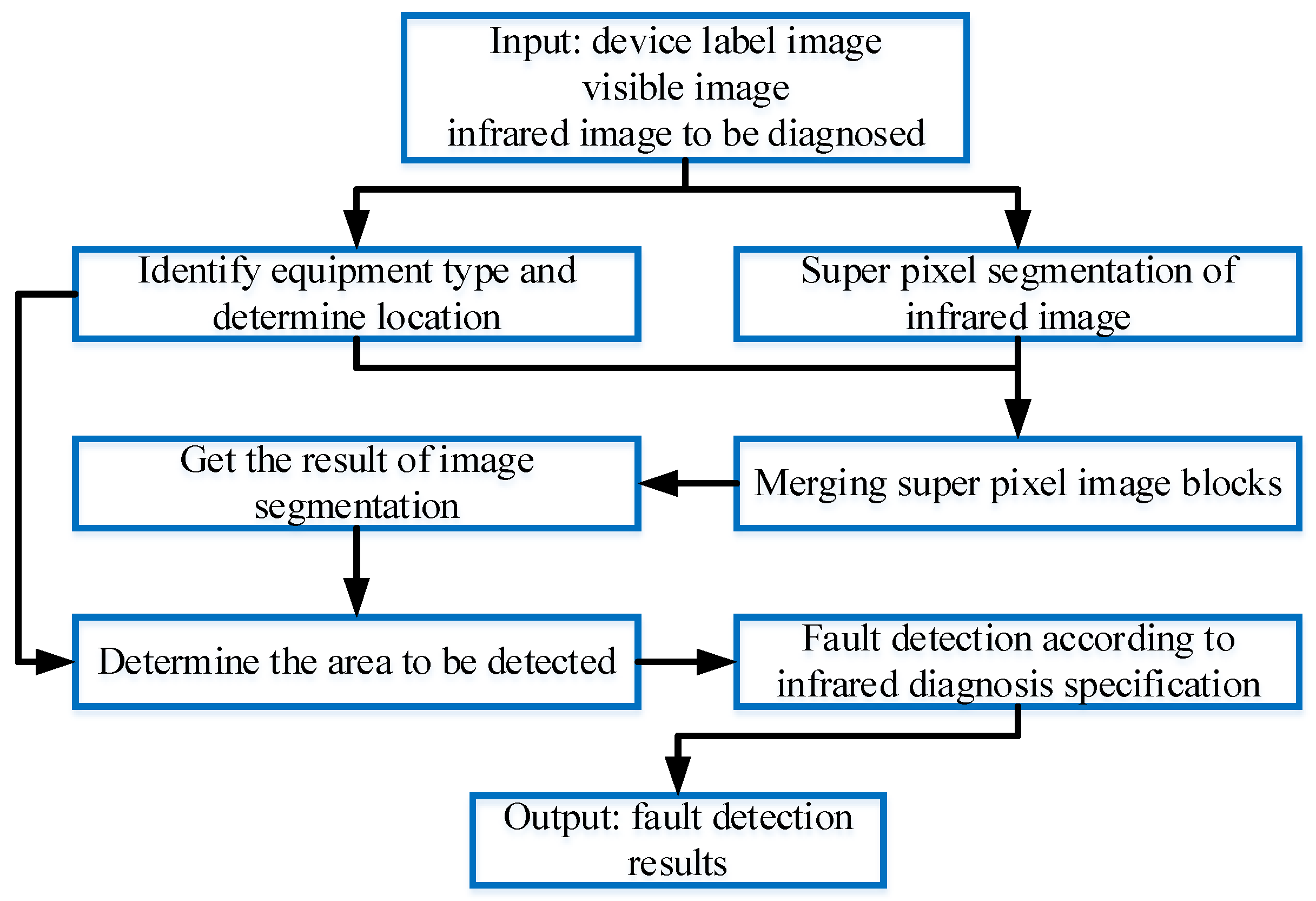
5. Experiment and Result Analysis

5.1. Experimental Data and Evaluation Paramenters

All the environments are carried out on a computer with Intel(R) Core (TM)i5-9300H CPU @2.40 GHz and 16.00 GB RAM. We debugged the following parameters on MATLAB: λ = 0.004 ; ε 0 = 0.008 ; γ = 2 . The HR image is composed of 32 × 32 blocks. A sparse dictionary, consisting of 3096 atoms of length 1024, is trained by the high-dimensional dictionary training method introduced in [26].
We compared our method with the methods proposed by Keys [30], Shao [19], Li [11], and Kim [21] and adopted the average gradient (AG) and information entropy (IE) as objective evaluation indicators.
In order to verify the actual application effect of the infrared image reconstructed by our proposed algorithm, we used the image recognition algorithm proposed in literature [31] to design a comparative experiment. Through the recognition of infrared images reconstructed by different SR methods, the performance and practical application value of our method was verified. Since the basis of the image recognition algorithm lies in the effective extraction and correct matching of image feature points, the number of feature points obtained by image extraction and the correct matching rate of feature points were used as evaluation indicators. In order to more clearly reflect the difference between the performance of different algorithms, we randomly selected 80 sets of feature point matching results for visual display.
In addition, we performed the same infrared image diagnosis process on the high-resolution images reconstructed by different SR algorithms. We sequentially performed super pixel segmentation, image recognition, super pixel merging, image segmentation, equipment area extraction, and equipment operating status diagnosis on the reconstructed infrared image. The super pixel segmentation and merging algorithm adopted the methods in the literature [32], and the image recognition still used the algorithm proposed in the literature [31]. The diagnostic process of infrared images is shown in Figure 4.

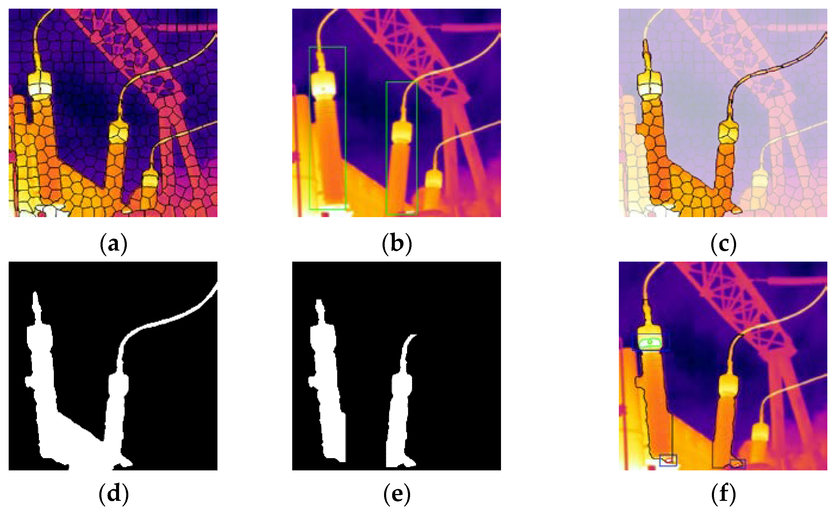
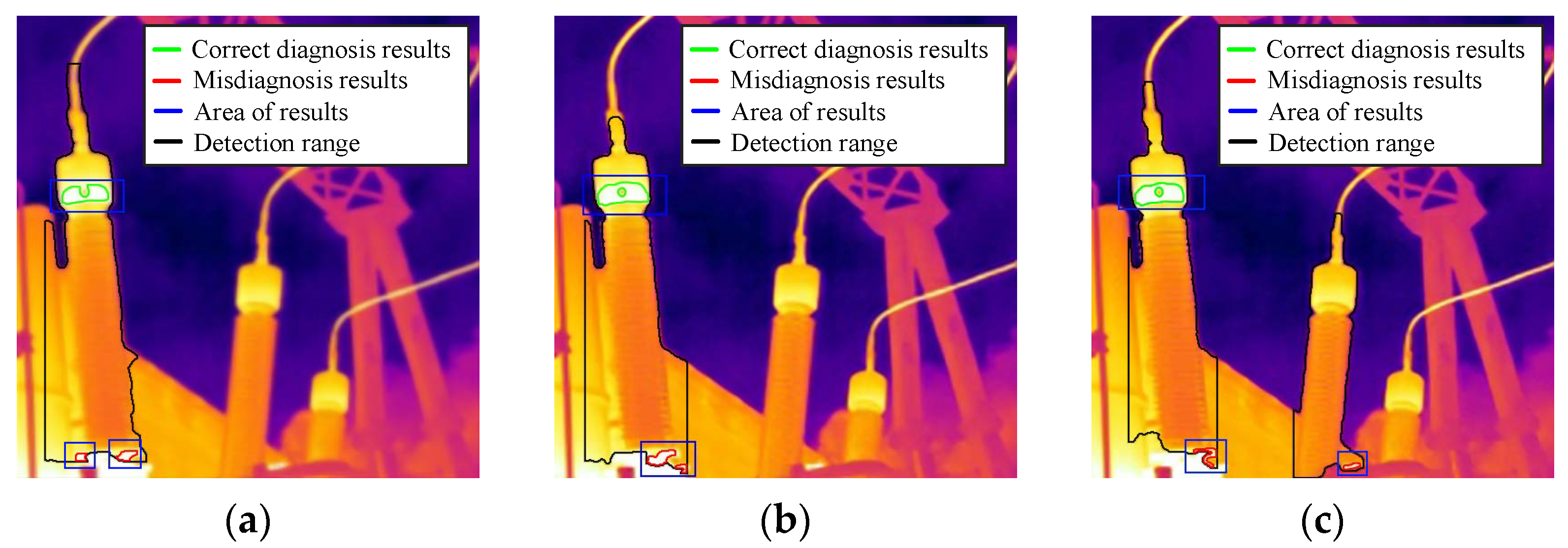
5.2. Infrared Image Reconstruction Experiment

We reconstructed low-resolution infrared images, thereby validating the effectiveness of our method in practical applications. We used 9 infrared images with a resolution of 128 × 128 taken on site for super-resolution reconstruction. The reconstruction results of image No. 9 using different methods are shown in Figure 5.
According to Figure 5, the reconstruction result of the method proposed by Keys et al. are the most ambiguous. The image details and textures reconstructed by the methods proposed by Shao and Li are similar. Although they have a significant improvement in visual quality compared to the original low-resolution blurred images, they are still blurry. The method proposed by Kim et al. reconstructed some significant textures of the image, but the textures have obvious defects. In addition, the image reconstructed by Kim et al. has poor visual quality, due to the ringing effect, but the AG indexes of the image are relatively high. However, the images reconstructed by our method are the sharpest. In summary, our method has certain advantages over current methods in handling blurred LR images. In addition, the blur kernel estimated by our method in the reconstruction process allows us to discover that image blur is very complex. It is inaccurate to use the standard Gaussian blur kernel to represent the image blurring process; that is to say, it is necessary to study the blind SR algorithm. The SR reconstruction results of the other eight infrared images by different methods are listed in Table 1 and Table 2 in the form of AG and IE metrics, respectively. It can be seen from the data in the tables that the reconstruction results of our method have certain advantages over these two indicators.

5.3. Comparative Experiment of Image Recognition

It can be seen from Figure 6 that the HR infrared image reconstructed by our proposed method has clearer and richer details. Therefore, the correct matching rate is significantly improved compared with the contrast method when performing feature point matching and recognition with the visible light sample image. Table 3 and Table 4 respectively show the number of feature points and the correct recognition rate of the infrared images reconstructed by different methods. The experimental results are mutually corroborated with Figure 6, which reflects the superiority of our method.

5.4. Comparative Experiment of Image Recognition

The intermediate results produced during the image diagnosis process are shown in Figure 7, Figure 8, Figure 9, Figure 10, Figure 11 and Figure 12, and the final diagnosis results are shown in Figure 13. It can be seen from Figure 13 that the detection area obtained by our method has the highest agreement with the actual device label image, and does not include the base of the transformer bushing. Compared with the actual device label image, the detection area obtained by other methods contains different degrees of the base of the transformer bushing. As a result, Figure 13b–e misdiagnosed the base of transformer bushing as a defective area of transformer bushing. According to the “Application rules of infrared diagnosis for live electrical equipment”, the diagnostic standards for different equipment are different. Since the bushing base is connected to the transformer tank, the internal oil temperature is relatively high, and the temperature of the bushing base is often higher than the surface temperature of the bushing. Therefore, the criteria for judging these two defects, i.e., “hot spot temperature or temperature difference” should be different. The image reconstructed by our method has clear edges, high contrast, and more obvious contours. Therefore, the image quality improvement of our method can improve the accuracy of equipment recognition, improve the accuracy of equipment area extraction, and improve the accuracy of defect diagnosis in the area to be detected in the infrared image diagnosis of equipment, thereby realizing accurate judgment of equipment operation.

6. Conclusions

Based on the background of the power Internet of Things, this paper presents a compression sensing super resolution method to solve the problem that the accuracy of infrared sensors is not enough to affect the accuracy of infrared diagnosis. A gradient norm ratio is used to improve the accuracy of blur kernel estimation, and a TwTVSI method is designed to achieve high-quality image reconstruction. The experimental part proves the effectiveness of the super-resolution method proposed in this paper.
In the era of the Internet of Things, the processing of infrared image data will be carried out automatically by computer. Our method can provide a good data base for the application of various algorithms, and has a broad application space. Firstly, the improvement of image quality by this method is helpful to the accurate operation of the image recognition algorithm. In the reconstructed image, the algorithm can identify more effective feature points and match them accurately, which is helpful to the classification and storage of infrared image data. Second, good image quality helps to improve the recognition accuracy of power equipment in the image. It can be seen from the experiment carried out in Section 5.4 that when image definition is insufficient, some transformer bushing cannot be accurately identified. Thirdly, the infrared image reconstructed by the super-resolution algorithm is more accurate in fault diagnosis, because the reconstruction results provide a good foundation for the image segmentation algorithm and can locate the equipment area more accurately. To sum up, the improvement of image quality by this method is helpful to the accurate realization of various practical applications based on infrared images of power equipment.
In addition, we believe that in the near future, when 5G communication, cloud computing and other technologies are further applied, the image data collected by infrared sensors will be analyzed on the cloud platform through cloud computing technology. After the operation and maintenance personnel obtain the access port of the cloud platform, they can accurately grasp the operation status of the equipment through mobile phones and computers anytime, anywhere, and then complete the operation and maintenance work according to the platform prompts. Our algorithm will have greater significance for image preprocessing, which could not only improve the accuracy of various algorithms based on equipment infrared images, but also provide clearer equipment observation conditions for operation and maintenance personnel.

Author Contributions

The conceptualization, data curation, formal analysis, and methodology were performed by Y.W. The software, supervision, formal analysis, validation, and writing—original draft preparation, review, and editing were performed by J.Z. and L.W. All authors have read and agreed to the published version of the manuscript.

Funding

This research was funded by National Natural Science Foundation of China, 51807063; and the Fundamental Research Funds for the Central Universities, 2021MS065.

Institutional Review Board Statement

Not applicable.

Informed Consent Statement

Not applicable.

Conflicts of Interest

The authors declare no conflict of interest.

References

  1. Lin, Y.; Zhang, W.; Zhang, H.; Bai, D.; Li, J.; Xu, R. An intelligent infrared image fault diagnosis for electrical equipment. In Proceedings of the 2020 5th Asia Conference on Power and Electrical Engineering (ACPEE), Chengdu, China, 4–7 June 2020; pp. 1829–1833. [Google Scholar]
  2. Li, X. Design of Infrared Anomaly Detection for Power Equipment Based on YOLOv3. In Proceedings of the 2019 IEEE 3rd Conference on Energy Internet and Energy System Integration (EI2), Changsha, China, 8–10 November 2019; pp. 2291–2294. [Google Scholar]
  3. Wang, Y.; Chen, Q.; Zhang, N.; Feng, C.; Teng, F.; Sun, M.; Kang, F. Fusion of the 5G Communication and the Ubiquitous Electric Internet of Things: Application Analysis and Research Prospects. Power Syst. Technol. 2019, 43, 1575–1585. [Google Scholar]
  4. Zhao, S.; Zhao, H.; Shou, P. Discussion on Key Technology and Operation & Maintenance of Intelligent Power Equipment. Autom. Electr. Power Syst. 2020, 44, 1–10. [Google Scholar]
  5. Lozanov, Y.; Tzvetkova, S. A methodology for processing of thermographic images for diagnostics of electrical equipment. In Proceedings of the 2019 11th Electrical Engineering Faculty Conference (EEFC), Varna, Bulgaria, 11–14 September 2019; pp. 1–4. [Google Scholar]
  6. Li, Y.; Zhao, K.; Ren, F.; Wang, B.; Zhao, J. Research on Super-Resolution Image Reconstruction Based on Low-Resolution Infrared Sensor. IEEE Access 2020, 8, 69186–69199. [Google Scholar] [CrossRef]
  7. Huo, W.; Tuo, X.; Zhang, Y.; Huang, Y. Balanced Tikhonov and Total Variation Deconvolution Approach for Radar For-ward-Looking Super-Resolution Imaging. IEEE Geosci. Remote. Sens. Lett. 2021, 19, 1–5. [Google Scholar] [CrossRef]
  8. Batz, M.; Eichenseer, A.; Kaup, A. Multi-image super-resolution using a dual weighting scheme based on Voronoi tessellation. In Proceedings of the 2016 IEEE International Conference on Image Processing (ICIP), Phoenix, AZ, USA, 25–28 September 2016; pp. 2822–2826. [Google Scholar]
  9. Wang, L.; Lin, Z.; Deng, X.; An, W. Multi-frame image super-resolution with fast upscaling technique. arXiv preprint 2017, arXiv:1706.06266. [Google Scholar]
  10. Rasti, P.; Demirel, H.; Anbarjafari, G. Improved iterative back projection for video super-resolution. In Proceedings of the 2014 22nd Signal Processing and Communications Applications Conference (SIU), Trabzon, Turkey, 23–25 April 2014; pp. 552–555. [Google Scholar]
  11. Li, L.; Xie, Y.; Hu, W.; Zhang, W. Single image super-resolution using combined total variation regularization by split Bregman Iteration. Neurocomputing 2014, 142, 551–560. [Google Scholar] [CrossRef]
  12. Kato, T.; Hino, H.; Murata, N. Multi-frame image super resolution based on sparse coding. Neural Networks 2015, 66, 64–78. [Google Scholar] [CrossRef]
  13. Greaves, A.; Winter, H. Multi-frame video super-resolution using convolutional neural networks. IEEE Trans Multimed. 2017, 8, 76–85. [Google Scholar]
  14. Hayat, K. Multimedia super-resolution via deep learning: A survey. Digit. Signal Process. 2018, 81, 198–217. [Google Scholar] [CrossRef] [Green Version]
  15. Dong, W.; Zhang, L.; Lukac, R.; Shi, G. Sparse representation-based image interpolation with nonlocal autoregressive model-ing. IEEE Trans. Image Process. 2013, 22, 1382–1394. [Google Scholar] [CrossRef] [Green Version]
  16. Wang, L.; Wu, H.; Pan, C. Fast Image Upsampling via the Displacement Field. IEEE Trans. Image Process. 2014, 23, 5123–5135. [Google Scholar] [CrossRef]
  17. Zhang, Y.; Fan, Q.; Bao, F.; Zhang, C. Single-image super-resolution based on rational fractal interpolation. IEEE Trans. Image Process. 2018, 27, 3782–3797. [Google Scholar]
  18. Manjón, J.V.; Coupe, P.; Buades, A.; Fonov, V.; Collins, D.L.; Robles, M. Non-local MRI upsampling. Med Image Anal. 2010, 14, 784–792. [Google Scholar] [CrossRef] [Green Version]
  19. Shao, Z.; Ge, Q.; Wang, Q.; Lin, Z.; Deng, S.; Li, B. Nonparametric Blind Super-Resolution Using Adaptive Heavy-Tailed Priors. J. Math Imaging Vis. 2019, 61, 885–917. [Google Scholar] [CrossRef]
  20. Yang, J.; Wright, J.; Huang, T.S.; Ma, Y. Image Super-Resolution via Sparse Representation. IEEE Trans. Image Process. 2010, 19, 2861–2873. [Google Scholar] [CrossRef]
  21. Kim, H.; Lee, S. Blind single image super resolution with low computational complexity. Multimed. Tools. Appl. 2017, 76, 7235–7249. [Google Scholar] [CrossRef]
  22. Wang, X.; Yu, K.; Dong, C.; Loy, C.C. Recovering Realistic Texture in Image Super-Resolution by Deep Spatial Feature Transform. In Proceedings of the IEEE Conference on Computer Vision and Pattern Recognition (CVPR), Salt Lake City, GA, USA, 17–19 June 2018; pp. 606–615. [Google Scholar]
  23. Zoph, B.; Le, V. Neural architecture search with reinforcement learning. arXiv preprint 2016, arXiv:1611.01578. [Google Scholar]
  24. Efrat, N.; Glasner, D.; Apartsin, A.; Nadler, B.; Levin, A. Accurate blur models vs. image priors in single image su-per-resolution. In Proceedings of the 2013 IEEE International Conference on Computer Vision (ICCV), Sydney, NSW, Australia, 1–8 December 2013; pp. 2832–2839. [Google Scholar]
  25. Donoho, D.L. Compressed sensing. IEEE Trans. Inf. Theory 2006, 52, 1289–1306. [Google Scholar] [CrossRef]
  26. Xu, L.; Lu, C.; Xu, Y.; Jia, J. Image smoothing via L0 gradient minimization. In Proceedings of the 2011 SIGGRAPH Asia Conference, Hong Kong, China, 13–15 December 2011; pp. 1–12. [Google Scholar]
  27. Zhang, H.; Hager, W.W. A Nonmonotone Line Search Technique and Its Application to Unconstrained Optimization. SIAM J. Optim. 2004, 14, 1043–1056. [Google Scholar] [CrossRef] [Green Version]
  28. Cho, S.; Lee, S. Fast Motion Deblurring. ACM Trans. Graph. 2009, 28, 1–8. [Google Scholar] [CrossRef]
  29. Wang, Y.; Wang, L.; Liu, B.; Zhao, H. Research on Blind Super-Resolution Technology for Infrared Images of Power Equipment Based on Compressed Sensing Theory. Sensors 2021, 21, 4109. [Google Scholar] [CrossRef] [PubMed]
  30. Keys, R. Cubic convolution interpolation for digital image processing. IEEE Trans. Acoust. Speech Signal Process. 1981, 29, 1153–1160. [Google Scholar] [CrossRef] [Green Version]
  31. Patel, M.I.; Thakar, V.K.; Shah, S.K. Image registration of satellite images with varying illumination level using HOG descriptor based SURF. Procedia Comput. Sci. 2016, 93, 382–388. [Google Scholar] [CrossRef] [Green Version]
  32. Chen, J.; Li, Z.; Huang, B. Linear Spectral Clustering Superpixel. IEEE Trans. Image Process. 2017, 26, 3317–3330. [Google Scholar] [CrossRef]
Figure 1. Reconstruction of high frequency information cost chart of image with different constraints: (a) high-frequency information is obtained by the transverse difference operator; (b) high-frequency information is obtained by longitudinal difference operator.
Applsci 12 04046 g001
Figure 2. The flow of the blur kernel estimation algorithm.
Applsci 12 04046 g002
Figure 3. Block diagram of TwTVSI algorithm [29].
Applsci 12 04046 g003
Figure 4. Flow chart of infrared image fault diagnosis.
Applsci 12 04046 g004
Figure 5. Different methods to reconstruct the real infrared image of No. 9. (a) Real infrared image (b) Reconstruction results using the method in [30] (AG = 20.705, IE = 6.222) (c) Reconstruction results using the method in [19] (AG = 28.421, IE = 6.323) (d) Reconstruction results using the method in [11] (AG = 28.452, IE = 6.362) (e) Reconstruction results using the method in [21] (AG = 31.559, IE = 6.429) (f) Reconstruction results using our method (AG = 30.784, IE = 6.542).
Applsci 12 04046 g005
Figure 6. Feature point matching results of infrared images reconstructed by different methods (a) LR (b) Keys’ (c) Shao’s (d) Li’s (e) Kim’s (f) Ours.
Applsci 12 04046 g006
Figure 7. The results of each step in the process of diagnosis by LR image (a) Super pixel segmentation (b) Image recognition (c) Super pixel binning (d) Image segmentation (e) Area to be inspected (f) Diagnosis result.
Applsci 12 04046 g007
Figure 8. The results of each step in the process of diagnosis by Keys’ method (a) Super pixel segmentation (b) Image recognition (c) Super pixel binning (d) Image segmentation (e) Area to be inspected (f) Diagnosis result.
Applsci 12 04046 g008aApplsci 12 04046 g008b
Figure 9. The results of each step in the process of diagnosis by Shao’ method (a) Super pixel segmentation (b) Image recognition (c) Super pixel binning (d) Image segmentation (e) Area to be inspected (f) Diagnosis result.
Applsci 12 04046 g009
Figure 10. The results of each step in the process of diagnosis by Li’s method (a) Super pixel segmentation (b) Image recognition (c) Super pixel binning (d) Image segmentation (e) Area to be inspected (f) Diagnosis result.
Applsci 12 04046 g010
Figure 11. The results of each step in the process of diagnosis by Kim’ method (a) Super pixel segmentation (b) Image recognition (c) Super pixel binning (d) Image segmentation (e) Area to be inspected (f) Diagnosis result.
Applsci 12 04046 g011
Figure 12. The results of each step in the process of diagnosis by our method (a) Super pixel segmentation (b) Image recognition (c) Super pixel binning (d) Image segmentation (e) Area to be inspected (f) Diagnosis result.
Applsci 12 04046 g012
Figure 13. Final diagnosis results of reconstructed images by different methods (a) LR (b) Keys’ (c) Shao’s (d) Li’s (e) Kim’s (f) Ours.
Applsci 12 04046 g013aApplsci 12 04046 g013b
Table 1. Comparison of AG indexes of images reconstructed using different methods.
Image NumberKeysShaoLiKimOurs
119.77527.04130.88429.34932.264
222.08829.50134.08032.24235.862
321.67329.86434.45435.39737.037
418.22420.51623.26725.40324.967
518.66326.54429.11328.80230.924
617.38225.65326.67126.23928.594
724.43634.37135.12537.53842.723
820.33526.41134.92927.21632.857
Table 2. Comparison of IE indexes of images reconstructed using different methods.
Image NumberKeysShaoLiKimOurs
15.5046.2036.1116.0486.276
26.5976.4196.6536.7066.948
36.3186.5816.7386.4426.281
45.5305.6035.7625.8915.806
56.1036.1436.2496.5436.698
65.6095.5815.6095.1915.792
76.7426.7646.8656.7826.876
85.7135.8625.7905.9835.316
Table 3. The number of feature points detected in images reconstructed by different methods.
Image NumberLRKeysShaoLiKimOurs
1257278351377385405
2219248309328334365
3153164210223221252
4256276351375379416
5185209267282292326
Table 4. The correct matching rate of feature points in images reconstructed by different methods.
Reconstruction AlgorithmCorrect Matching Rate of Feature Points
Image 1Image 2Image 3Image 4Image 5
LR52.3848.7851.1550.2253.79
Keys’55.9550.7052.3753.8454.34
Shao’s61.5259.5664.5661.8864.75
Li’s71.0371.7671.7969.7570.91
Kim’s74.2372.6276.6576.3674.48
Ours82.1383.4081.0483.2584.21
Publisher’s Note: MDPI stays neutral with regard to jurisdictional claims in published maps and institutional affiliations.

