Detecting Deepfake Voice Using Explainable Deep Learning Techniques

Abstract

Fake media, generated by methods such as deepfakes, have become indistinguishable from real media, but their detection has not improved at the same pace. Furthermore, the absence of interpretability on deepfake detection models makes their reliability questionable. In this paper, we present a human perception level of interpretability for deepfake audio detection. Based on their characteristics, we implement several explainable artificial intelligence (XAI) methods used for image classification on an audio-related task. In addition, by examining the human cognitive process of XAI on image classification, we suggest the use of a corresponding data format for providing interpretability. Using this novel concept, a fresh interpretation using attribution scores can be provided.

1. Introduction

With recent advances in artificial intelligence and its applications, cases of abuses of AI technology have also increased. A deepfake is one of the main methods that powers many of such cases. Thus far, only a few celebrities have been targeted. However, owing to two phenomena triggered by the public’s recent increased use of social media, i.e., (1) ease of data collection and (2) enhanced influence of information distribution, fake media has proliferated.

While deepfake generation has improved considerably in recent times, the accuracy of deepfake detection has remained at 82.56% when tested upon a public open dataset [1]. Though this performance improvement is significant from an academic perspective, it is still insufficient for real-world usage. Given two major emerging issues, i.e., less-than-perfect accuracy of detection and widened target range, interpretability of deepfake detection has become a critical consideration. However, contemporary research on explainable deepfake detection is not extensive and is limited to visual deepfake detection [2].

In this study, we implemented XAI methods on deepfake voice detection in order to be able to recommend the proper delivery of the interpretation at a human perception level. To target the non-experts for linguistics as well as artificial intelligence, the study is focused on intuitiveness and a higher level of interpretability.

Currently, for speech recognition or speaker verification, methods, such as transformers, conformers, or wav2vec, already show good performance [3,4,5]. However, in this study, to focus on the proper delivery of the interpretation rather than the performance, simple model structures are used. A simple convolutional neural network and LSTM were used to maintain as much simplicity as possible.

A spectrogram was used for feature extraction from the raw audio data. A spectrogram requires relatively less preprocessing and is easily interpretable. Features, such as d-vector, x-vector, or i-vector already show satisfactory performances for tasks, such as speaker verification. However, such feature embeddings are excluded because direct interpretability with the original audio data are lost [6,7,8].

For our experiment, the ASVspoof 2019 Logical Access and LJSpeech datasets were used, each exclusively representing a near real-world dataset and constrained dataset [9,10]. ASVspoof consists of bona fide user speech along with synthesized speech generated through multiple generators. We labeled bona fide speech as a ‘human voice’ and completely synthesized voice as a ‘deepfake voice’. As a constrained dataset, we used LJSpeech, and synthesized speeches based on it. We labeled the original LJSpeech speech as a ‘human voice’ and the Tacotron-generated speech as a ‘deepfake voice’.

To maintain as much simplicity and interpretability as possible, three CNN-based simple model structures were used for the experiment: CNN, CNN-LSTM, and CNN-LSTM-permuted. To analyze the trained model, popular XAI methods, such as Deep Taylor, integrated gradients, and layer-wise relevance propagation (LRP) were used [11,12,13]. For the CNN-based simple model, all three XAI methods showed similar attribution score distributions, with high absolute values located on formants 1, 2, and 3. As an LSTM layer was added to the model, Deep Taylor and LRP were no longer dependent on the formants. Deep Taylor shows that dependency varies on the frequency bands and LRP shows characteristics that cannot be recognized through human visual perception.

Audiovisual Interpretability

Traditionally, audio has been analyzed through spectrograms extracted from raw audio by Fourier transform [14]. For a human voice, the analysis is made using a mel spectrogram, which filters the spectrogram through a mel filterbank to emphasize low-frequency spectra in which most of the energy is concentrated [15]. Tasks, such as speaker verification, use x-vector or d-vector to make the process efficient [6,7]. However, the requirement of domain knowledge and absence of interpretability made the use of spectrograms and embedded vector features, respectively, less suitable for non-experts.

For human manual analysis, visualized audio data in the form of a spectrogram is traditionally used [16]. Characteristics, such as distribution of the energy, formant, frequency-wise characteristics, or general waveform are used for the analysis. However, recognizing these characteristics requires more than just intuitive human perception. The need for domain knowledge makes this method less user-friendly for non-experts compared to visual data-related tasks. Owing to the following two reasons, we achieved effectiveness of interpretability with the corresponding format: (1) lack of intuitive recognition based on visualized interpretability, and (2) tendency of the XAI methods observed on image classification. As a means of converting visualized interpretation back to audio, we used the Griffin–Lim algorithm.

On CNN-based simple models, regardless of the XAI methods used, the attribution scores show energy dependency on the spectrogram. Given the tendency of the scores, the attribution-score-based recomposed audio is audible. When an LSTM layer is added, Deep Taylor loses its energy dependency and makes the transcript of the recomposed audio unrecognizable but shows significant differences between human and deepfake voices on rhythm and pitch variances. In general, a deepfake voice shows relative monotonousness.

The major contribution of this paper is that it suggests two novel ideas on deepfake detection, i.e., adaptation of XAI for spoken language and multi-modal interpretability at a human perception level. Visual and audio interpretation, respectively, enabled interpretation of model tendency on general spoken language data and intuitive recognition of characteristics that are not effortlessly recognized when only visual interpretation is available.

The remainder of the paper is organized as follows. In Section 2, we introduce related works, i.e., explainable deepfake image detection and explainable speech recognition. In Section 3, preliminaries and datasets are described. In Section 4, methods and motivations are introduced along with the experimental environments. In Section 5, we suggest interpretation based on the attribution score of the model. Finally, in Section 6, the study is summarized along with its limitations and future research directions.

2. Related Works

Currently, application of XAI is in the early stage; the methods were introduced in the mid-2010s. Most implementations on deepfake detection methods are focused on image recognition. Although there has been attempt to joint both visual and audio data to detect the deepfake, the interpretation on the model has not been tried [17]. A recent study implemented LIME and LRP to provide interpretability only for visual deepfake detection [2]. For deepfake facial images, XAI methods provide a heatmap for the trained model to suggest the regions to focus on.

Implementation of XAI on speech recognition rather than both visual and audio deepfake detection is scant, but it exists; the same XAI method, LRP, is commonly used to provide interpretability. A study by Bharadhwaj suggested a bidirectional-GRU-based model built for the implementation of XAI methods and finding the relevance score for each input [11]. Through perturbation comparison, they suggested the superiority of bi-GRU over uni-GRU, LSTM, and bi-LSTM. Becker et al. compared the implementation of LRP on speech recognition with two tasks: digit classification and gender classification [18]. Each task was trained with AlexNet and compared using the LRP attribution score. Along with the comparison, the authors proved the meaningfulness of LRP on speech recognition through data perturbation.

These studies focused on quantitative evaluation of the XAI methods on spoken language processing. Though the studies shared some ideas, our study focuses on qualitative evaluation.

The XAI methods applied to various tasks, yet focused on image related tasks, such as layer-wise relevance propagation or Deep Taylor decomposition, provide intuitive model interpretations with a form of a heatmap. The interpretation can be effortlessly obtained without modifying the existing trained model. The generic idea of such Taylor decomposition-based XAI methods is to trace back the contribution of every input for each trained node to the final prediction layer-by-layer. By iteratively calculating the contribution of every node, the model can be interpreted pixel-by-pixel, which is a heatmap of the input image.

Although interpretability adoptable to the existing trained model is significant, as Jung et al. mentioned, the methods show limitations: high noise of heatmap output and lack of class-discriminativeness [19]. Considering such limitations, we found it necessity to interpret at the human cognitive level. By focusing on qualitative evaluation of the interpretation, noise of the heatmap can be overcame through the human cognitive level of contextual interpretation. Hence, based on the interpretation to the human-in-loop system as a guideline, lack of class-discriminativeness is also expected to be efficiently resolved.

3. Preliminaries and Dataset

3.1. Deepfake

Deepfakes are synthesized media generated using deep learning methods, such as a generative adversarial network or autoencoder. In real-world applications, it is often used in a form of face-swapping. Face-swapping involves an encoder and a decoder that representatively learn target and base face as well as transforms. Deepfake voices are generally divided into two categories: text-to-speech (TTS) generation and voice conversion. TTS generation only trains the model for audio generation using a text transcript as input, while voice conversion is voice-to-voice conversion, similar to face-swapping. Currently, both generation methods show good performance, so lay viewers are usually unable to distinguish between the real and deepfake media intuitively.

3.2. Speech Analysis

Speech can be categorized into three types: voiced, unvoiced, and silence. Voiced speech has constrained energy with a periodic impulse sequence, while unvoiced speech is a relatively random non-periodic noise-like sequence. Silence refers to a section with no meaningful signals.

For categorized speeches, several linguistic features, including formant, are used for analysis. Formant is the frequency with constrained energy, showing a local maximum on the spectrum. For general human speech, three to five formants can be found, and named in ascending order from low-frequency formant to high. In voiced and unvoiced speech, the first three formants form the mainframe of the speech, considered as one of the representative features.

In voiced speech, pitch and amplitude are also considered major features. These two voiced speech features represent expressions of stress and the accent of the speech. In unvoiced speech, the local center frequency and its amplitude at high frequency are considered key features.

Based on such acoustic information, speech recognition or speaker recognition can be performed through human or algorithm analysis. In this study, for a higher level of interpretation, such traditional features are used to interpret the attribution scores acquired from the XAI methods applied to the detection models.

3.3. Dataset

For the general interpretation of the detection model, two datasets with exclusive characteristics were used. The first set of experiments was conducted upon the ASVspoof 2021 Logical Access dataset. ASVspoof consists of 2580 bona fide user speech data collected from 107 speakers and the corresponding 22,800 synthesized speech data generated using 19 synthesizers. We labeled the bona fide user voice and synthesized voice as the ‘human voice’ and ‘deepfake voice’, respectively. With various human speakers and randomly sampled transcripts for text inputs of deepfake voice generation, the experimental environment was able to represent near real-world behavior.

For the constrained environment, paired data for both human and deepfake voices was required. We used the LJSpeech dataset consisting of 13,100 transcripts and speeches and generated the corresponding deepfake speeches. With the LJSpeech dataset, we used Tacotron, an attention-based sequence-to-sequence TTS generator to train the generation model [20]. From the complete dataset, we selected 8076 speeches and prepared the corresponding synthesized speeches. LJSpeech speech and synthesized speech were, respectively, labeled and trained as ‘human voice’ and ‘deepfake voice’.

4. Methods

4.1. Motivation

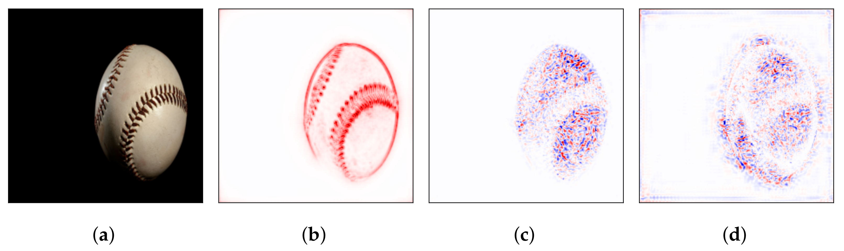
As mentioned earlier, visualized interpretation with XAI methods for image classification that provides the output in the form of a heatmap is often acceptable. If the classification accuracy is high enough, the ensuing XAI result also tends to proceed properly. However, current XAI methods are not perfect, and often fail to separate an object from the background, eventually only highlighting the high-contrast object contour. Figure 1 shows the input image and its attribution score obtained using three XAI methods for image classification based on VGG16 trained upon ImageNet data. Deep Taylor shows the positive score distribution on the high-contrast object contour. Integrated gradients and LRP show relatively random positive–negative score distributions, yet still highlight the general contour of the ball. However, when humans attempt to interpret such XAI output, visual perception is involved and assists in interpretation. Visual perception expects general or partial shapes of certain possible candidates and processes the attribution score of each pixel accordingly rather than as individual numbers. The involvement makes interpretation possible, despite the random negative score distribution near the contours. Such a series of phenomena can be seen as an interference of human visual perception caused by the difference in cognition levels between a human and machine (or model). Although there are several studies focusing on object segmentation, interference of human perception is inevitable until perfect segmentation is achieved [21].

Based on the difference between human and machine perception on image classification, we attempted to interpret the attribution score obtained from deepfake voice detection. We focused on the general distribution of the scores for contextual information following human perception and compared it with the traditional method used for the spectrogram-based audio analysis.

4.2. Feature Extraction

Through the Fourier transform, a complex signal can be sorted into multiple spectra at various frequencies [14]. Such a converted form is used for audio or video analyses. For audio analysis, the amplitude of each frequency of the audio wave is analyzed using a certain window size. The series of spectra are converted into a visualized form: a spectrogram. Using a spectrogram for the analysis, characteristics, such as general waveform and voiced-unvoiced-silenced frames, can be visually inspected by humans.

Generally, short-term Fourier transform is used to convert a audio signal into a two-dimensional function of time and frequency. The representation can be shown as follows:

$$\mathrm{STFT}(\tau ,\omega )={\int }_{-\infty }^{\infty }x\left(t\right)w(t-\tau )\exp (-iwt)dt$$

(1)

where $x\left(t\right)$ is the audio signal and $w\left(\tau \right)$ is the window function. For the window function, the Hann window is used [22].

Specifically, for human voice analysis, a mel spectrogram is used. Humans do not recognize audio in a linear scale; instead, they focus on low frequencies. Considering this characteristics of human perception, voice analyses traditionally use a mel-filterbank to convert a spectrogram into mel-scale. In this study, visual and audio interpretation was provided using spectrogram-based attribution scores in both visual and audio formats.

4.3. Models

Generally, speech recognition tasks using machine learning have spectrogram-based features as input data. The task of deepfake voice detection is similar to speaker recognition. Features used for speaker verification, such as x-vector or i-vector, show better performance and higher efficiency. However, because of the limitation of embeddings for providing interpretability, spectrogram-based features are used instead.

From the extracted mel spectrogram, we trained the recognition model using widely used networks. By applying several XAI methods to the model, we found general as well as distinguishing learning tendencies and interpreted them using the higher, human cognitive level of concept.

4.3.1. Convolutional Neural Network

A convolutional neural network (CNN) is one of the neural networks used for analyzing image data. As it can preserve contextual information, currently CNN is also used for extracting features in general. CNNs consist of convolution layers and pooling layers, which respectively learn feature vectors using an activation function and decrease the size of the data, making it relatively representative.

4.3.2. Long Short-Term Memory

Though the audio was converted to visualized data, i.e., a spectrogram, it still had time-series characteristics, unlike other visualized data. Consequently, a sequential model often used for spoken or natural language processing was used.

A sequential model, recurrent neural network, before LSTM, had a vanishing gradient problem. Adding cell-state to a hidden state LSTM resolved this issue. For overall sequential data and tasks, LSTM shows good results.

With two widely used simple networks, we set three models as listed in

Table 1. Model Structure.

CNN	CNN-LSTM	CNN-LSTM-Permuted
Input	Input	Input	Input (perm)
Conv1	Conv1	Conv1	Conv2
	LSTM1	LSTM1	LSTM2
FC-256	FC-256	FC-256
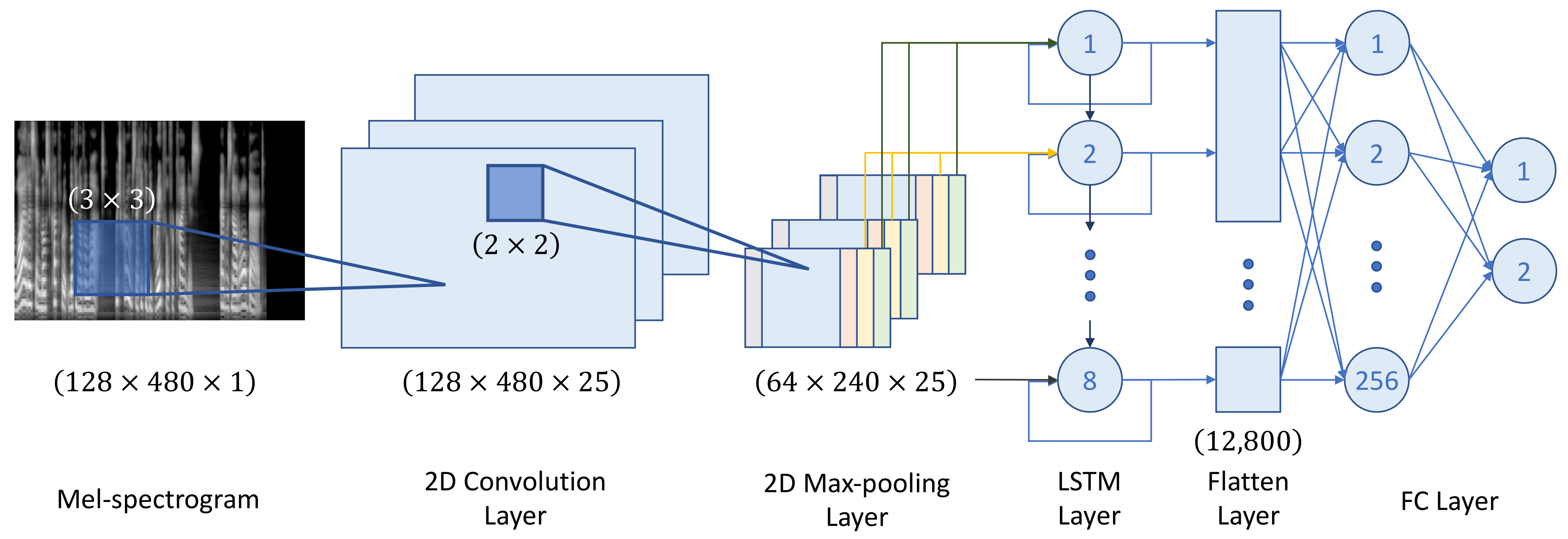
FC-25	FC-2	FC-2

. Considering the purpose of the experiment, we focused on simplicity rather than accuracy. As a representative, the structure–processing workflow for the CNN-LSTM model is shown in Figure 2. For all convolutional layers, ReLU was used as an activation function, and the kernel size was set to 3 × 3 with a stride of 1 and max-pooled with a kernel size of 2 × 2 with a stride of 1. All models feature FC-256, a fully connected dense layer. For the last FC layer for the classification between a real human voice and deepfake voice, softmax was used.

For ASVspoof dataset, four subsets configured by the generation methods of the deepfake voice were used for the experiment. For LJSpeech, human speeches with corresponding deepfake voices generated with Tacotron were used. Each subset was randomly divided into 80% of training data, 10% of validation data, and 10% of test data. The model was trained with the Adam optimizer for 100 epochs at a batch size of 50 speeches. The learning rate was set to 0.001.

4.4. Explainable Artificial Intelligence

Until recently, most AI research focused on its performance. With the application of evolving technology to the field, transparency become more critical. Unlike traditional simple algorithms, the complexity of artificial intelligence required a new approach. For a post-hoc approach, methodologies, such as decomposition and data perturbations, are now in use. In this study, we used layer-wise relevance propagation, Deep Taylor, and integrated gradients.

4.4.1. Integrated Gradients

The performance of an attribution method is generally evaluated in terms of accuracy drop by data perturbation with a high attribution score. However, the accuracy drop evaluates correlation rather than causality, which can be triggered by external factors. To evaluate properly, integrated gradients consider two axioms: sensitivity and implementation of invariance. Path integral can consider a non-linear path and integrate multiple attribution methods, resulting in adequate attribution evaluation. With the path integral formulation, integrated gradients can satisfy the axioms and properly calculate the attribution score [13].

For neural network, suppose there is a function $F:{\mathbb{R}}^n\to [0,1]$ with $x\in {\mathbb{R}}^n$ and $x^{\prime }\in {\mathbb{R}}^n$, respectively, as the input and the baseline input. By accumulating the gradients for all inputs, the integrated gradients can be obtained. It was calculated with the path integral of the gradients between input x and baseline input $x^{\prime }$, as followings:

$${\mathrm{IntegratedGradients}}_i::=(x_i-x_i^{\prime })\times {\int }_{\alpha =0}^1\frac{\partial F(x^{\prime }+\alpha \times (x-x^{\prime }))}{\partial x_i}\mathrm{d}\alpha$$

(2)

where $\frac{\partial F\left(x\right)}{\partial x_i}$ is the gradient of the function $F\left(x\right)$ on dimension i and $\alpha$ is the interpolation constant for the perturbation of the features.

4.4.2. Taylor Decomposition-Based XAI Methods

Several XAI methods use visual approaches to explain a model prediction for image classification or natural language processing. These methods generate a heatmap over the input data to highlight the relevance of the input to the prediction. Using three main ideas, relevance-based XAI methods calculate the score as follows: (1) all nodes at each layer have a certain amount of relevance; (2) the relevance is redistributed in a top–down direction from output to input of the node; and (3) the total amount of the relevance score on each layer is maintained. With the series of redistribution, the relevance score of each input data can be collected from the prediction.

For the decomposition of a given function, $f\left(x\right)$, and calculating each relevance score of input $x_i$, Taylor series is used. With the first-order Taylor series, $f\left(x\right)$ can be defined as follows:

$$f\left(x\right)=f\left(a\right)+\sum _{i=1}^d\frac{\partial f}{\partial x_i}{|}_{x_i=a_i}(x_i-a_i)+ϵ$$

(3)

where a is an arbitrary constant and $ϵ$ is the error term. Respectively, by the $w^2$-rule and property of ReLU, $f\left(a\right)$ and $ϵ$ can be approximated to 0. With the approximation, $f\left(x\right)$ can be defined as

$$f\left(x\right)=\sum _{i=1}^d\frac{\partial f}{\partial x_i}{|}_{x_i=a_i}(x_i-a_i)$$

(4)

$$=\sum _{i=1}^d{R}_i$$

(5)

where $\frac{\partial f}{\partial x_i}$ represents the relevance of $x_i$ for function f. By iteratively decomposing the outputs into the sum of relevance score of the input for every node, the heatmap of the prediction can be obtained.

4.5. Speech Reconstruction with the Griffin–Lim Algorithm

The Griffin–Lim algorithm is an algorithm generally used as a phase reconstruction rule-based vocoder before the neural vocoders [22]. It uses the redundancy of short-time Fourier transform with two projections of the spectrogram. The Griffin–Lim algorithm only utilizes the consistency of short-time Fourier transform and excludes any prior information. The algorithm reconstructs the spectrogram with a given amplitude A to the audio signal by the following process:

$$X^{[m+1]}=P_C\left(P_A\left(X^{\left[m\right]}\right)\right)$$

(6)

where $X^{\left[m\right]}$ is a spectrogram at iteration m, $P_C$ and $P_A$ are metric projections of the set of the consistent spectrogram and spectrogram with a given amplitude. The metric projections are given as:

$$P_C\left(X\right)=\mathrm{G}{\mathrm{G}}^{†}X$$

(7)

$$P_A\left(X\right)=A\odot X\oslash \left|X\right|$$

(8)

where G and ${\mathrm{G}}^{†}$ represent, respectively, short-time Fourier transform and inverse short-time Fourier transform. The optimization problem of the Griffin–Lim algorithm is obtained as following:

$$\underset{X}{\min }\left|\right|X-P_C\left(X\right){\left|\right|}_{\mathrm{Fro}}^2\mathrm{s}.\mathrm{t}.X\in A$$

(9)

where $\left|\right|·\left|\right|$ is the Frobenius norm. With the optimization by iteration, the spectrogram converges. Although various other reconstruction algorithms or neural vocoders are available, because of its simplicity, the Griffin–Lim algorithm is adopted instead. In this study, we considered the attribution score as a spectrogram and recomposed it back to audio to intuitively confirm the possible characteristics.

Considering the general behavior of the attribution scores on energy, the attribution score was expected to reflect the general form of the originating audio and its spectrogram. This greediness was also found in image classification, highlighting seemingly random positive–negative attribution scores mostly on the high-contrast contour, regardless of the object-background segmentation. Despite less-than-perfect segmentation, the interference of human visual perception enables XAI methods to provide interpretability. We were inspired to apply the idea of current XAI methods assisted with human perception, which have been used on visual tasks as well as audio tasks.

5. Experiment

In this section, we interpret the output of the three XAI methods. Each XAI method shows consistent results under several environments along with two noticeable differences.

Mel-spectrogram and the corresponding attribution score were reviewed as visualized data. Then, using the attribution score, we recomposed it back to audio and inspected it using an acoustic approach. By matching the data and interpretation format, the characteristics formally unrecognized solely via visual interpretation were revealed. The sample data were selected from the test set of each experimental environment.

For ASVspoof dataset, four subsets were used as follows:

• Deepfake voice generated by a single TTS model;
• Deepfake voice generated by multiple TTS models;
• Deepfake voice generated by a single voice conversion model;
• Deepfake voice generated by multiple voice conversion models.

5.1. Model Detection Performance

A model performance of each environment is summarized in

Table 2. Model Performance.

Model	Dataset
	ASV Single TTS	ASV Multiple TTS	ASV Single VC	ASV Multiple VC	LJSpeech
CNN	97.32%	77.78%	77.93%	83.61%	98.88%
CNN-LSTM	98.91%	88.74%	86.90%	84.81%	99.92%
CNN-LSTM-perm	99.85%	99.97%	94.19%	88.29%	99.97%

. Under certain environments, the model shows relatively less ideal performance. However, the primary goal of the experiment was to provide an interpretation rather than to achieve an improved performance. The performances were only used to confirm the proper model training for each environment. The ASVspoof-based model trained to detect the deepfake voice generated with multiple methods showed a generally low performance.

5.2. Visual Interpretability

5.2.1. ASVspoof Dataset

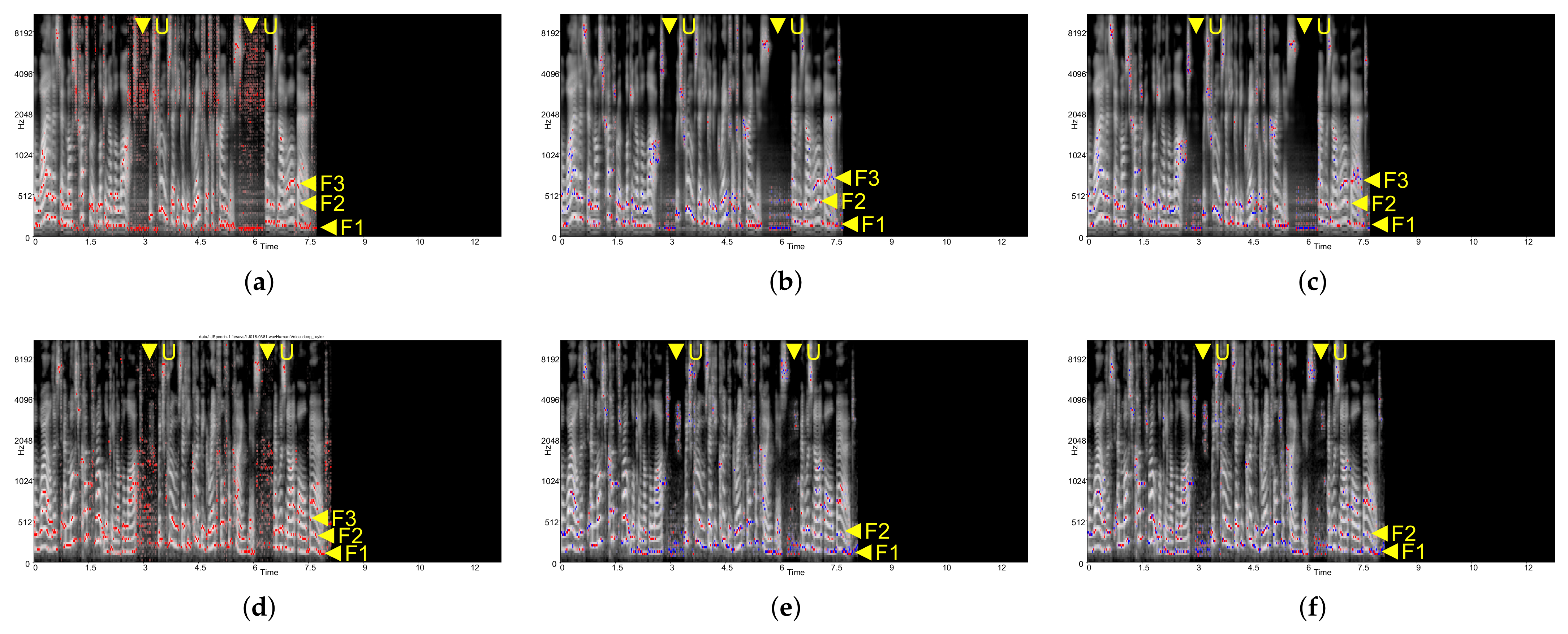
In Figure 3, all XAI methods for the CNN-based model highlight formants 1, 2, and 3, respectively, around areas F1, F2, and F3 of each figure. In acoustics, a formant is the local maximum or broad peak, similar to contours of objects as well as the background for visual content. For human speech, these first three formants are used to identify the vowel that is the fundamental component of the spoken language. In Figure 3a,d, Deep Taylor highlights the general formants 1, 2, and 3 while distinguishing unvoiced speeches by highlighting the corresponding frames at all frequencies around the area U.

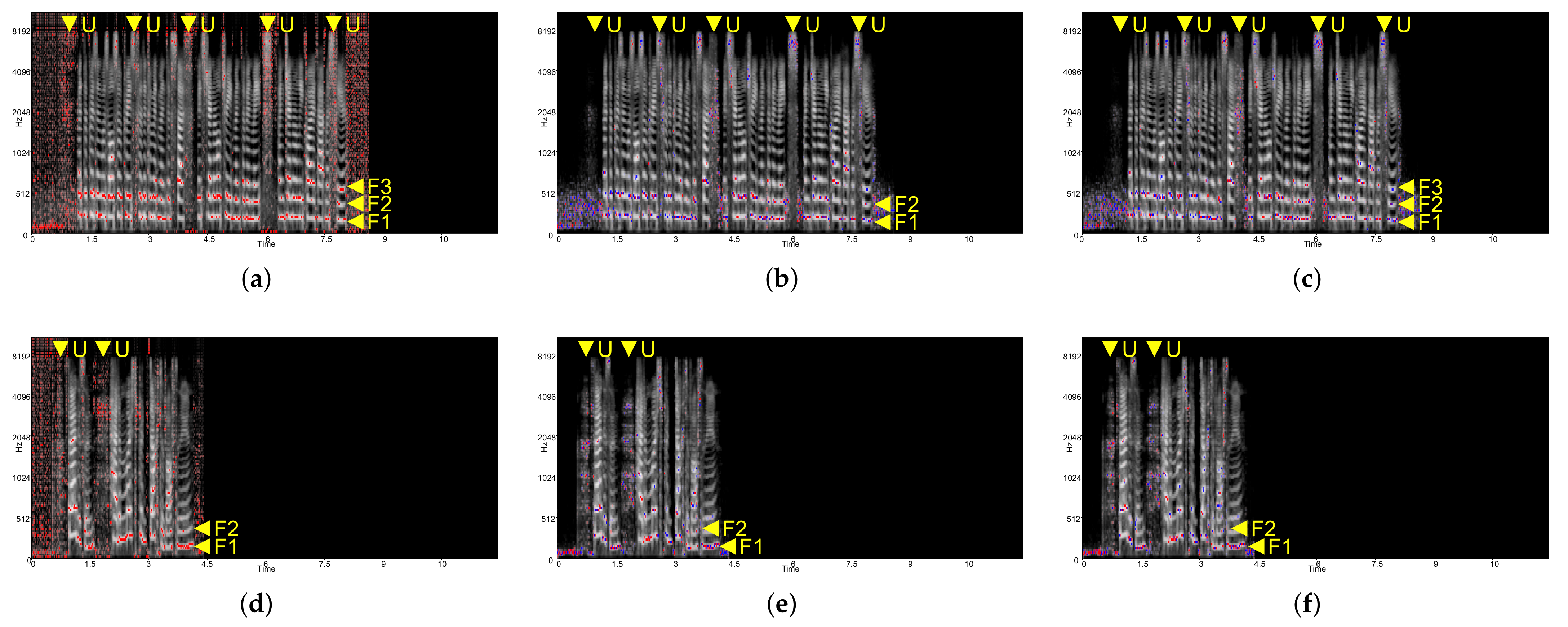
Figure 4 shows the result for each XAI method applied to the CNN-LSTM-based model. Only in Figure 4b,e, do the integrated gradients highlight the formants similar to the CNN-based model in Figure 3. In Figure 4a,d, Deep Taylor does not highlight the formants and unvoiced speeches. Instead, certain frequency bands are highlighted regardless of energy distribution from 0 to 500 Hz, and 1000 Hz to 2000 Hz, respectively, around areas A and B. In Figure 4c,f (LRP), though, the attribution score is no longer formant-dependent, unlike Deep Taylor, and it becomes less recognizable at the human cognitive level.

To see the frequency-wise series data characteristic of the model, CNN-LSTM-perm was used. Only Deep Taylor showed a difference—showing that less significant frequency band centered scoring was weakened. For integrated gradients and LRP, no recognizable difference was observed.

5.2.2. LJSpeech-Based Dataset

Although interpretation of the model based on the ASVspoof dataset showed the possibility of interpretation, a near-real-world dataset without paired transcripts over labels obstructed thorough interpretation. For better interpretation by XAI methods and model structures, the constrained dataset LJSpeech, which featured a single speaker and pre-defined transcript, was used.

In Figure 5, the CNN-only model trained with LJSpeech showed no significant difference compared to the model trained with ASVspoof. Similar to ASVspoof dataset, generally, the model tended to focus on formants 1, 2, and 3 around areas F1, F2, and F3, and unvoiced frames around area U when analyzed with Deep Taylor.

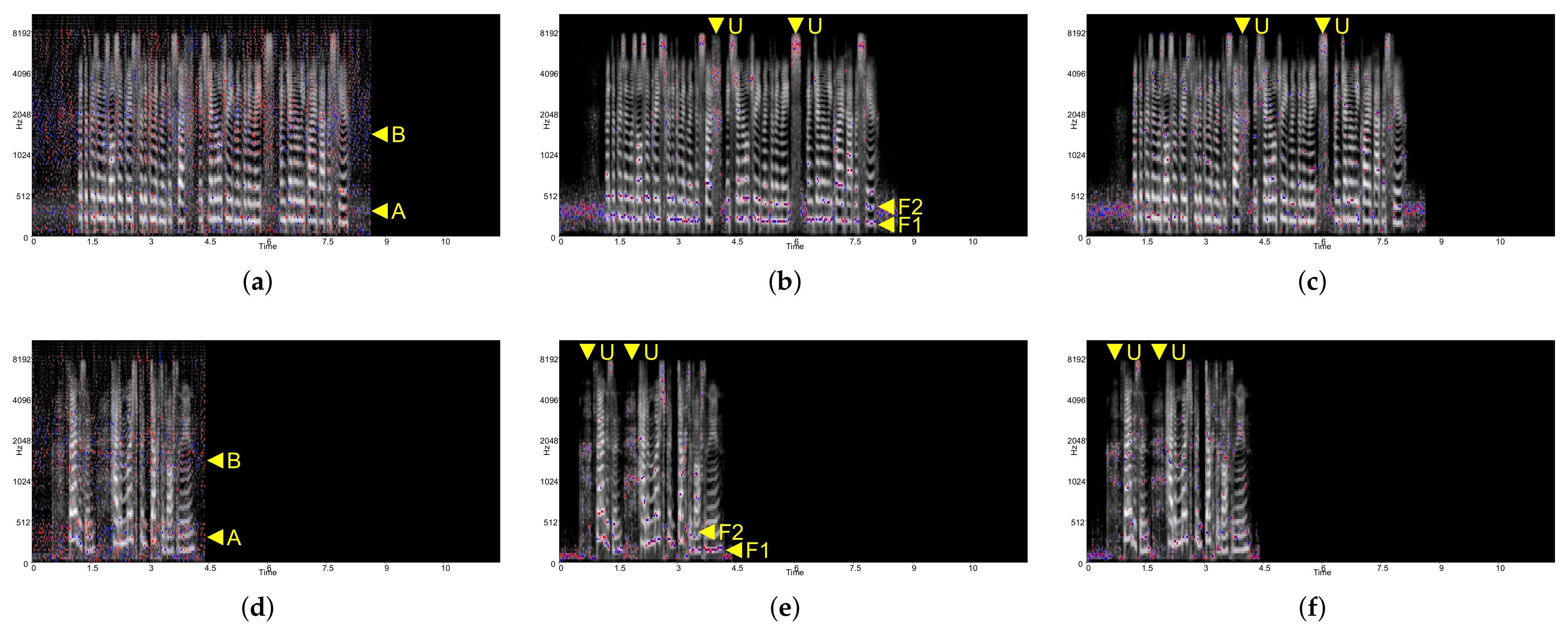
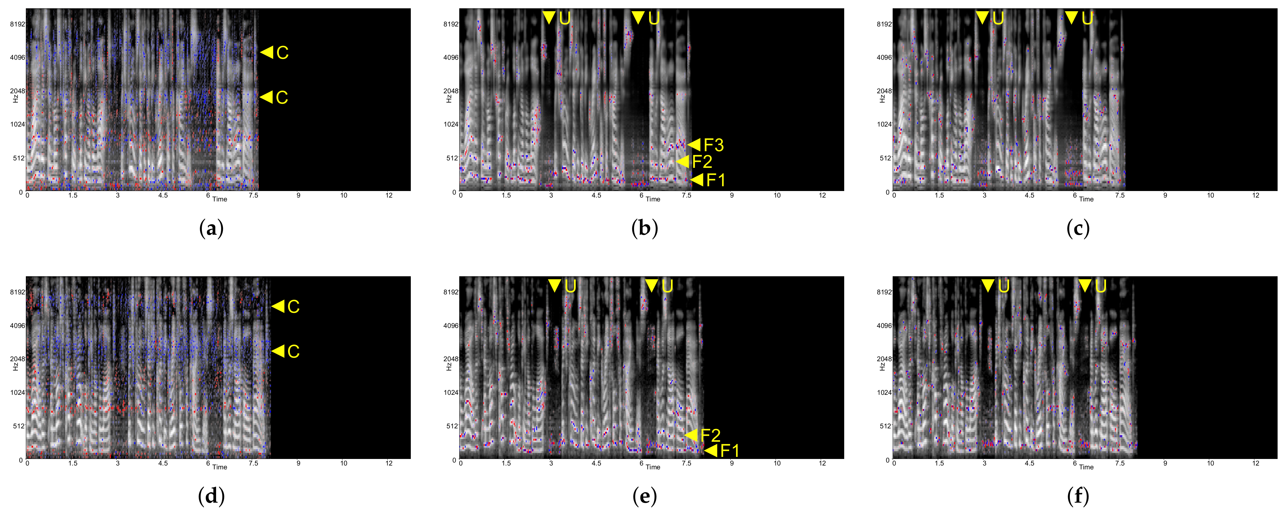
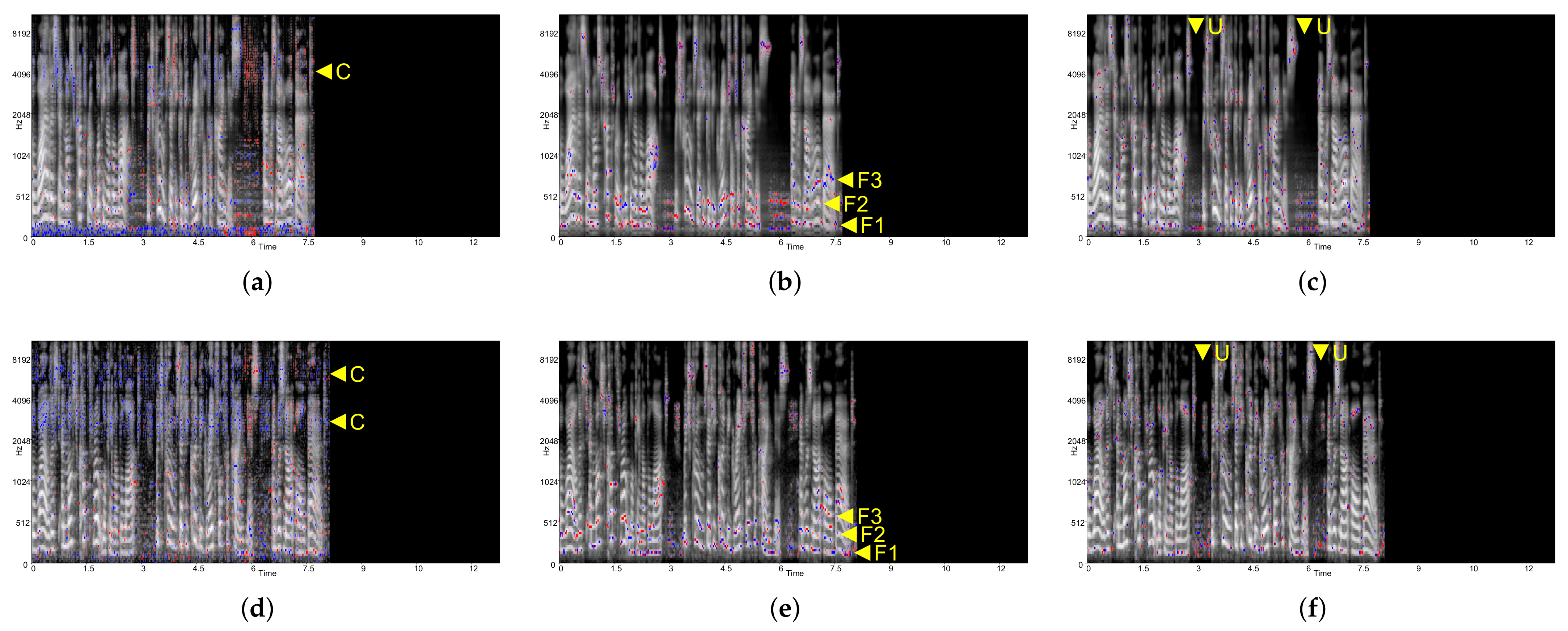
Similarly, in Figure 6 (CNN-LSTM) and Figure 7 (CNN-LSTM-perm), the formant dependency for Deep Taylor and LRP was diminished, as the previous ASVspoof-trained model has demonstrated. For Deep Taylor in Figure 6a,d, an identical model tendency on the frequency band found on ASVspoof was observed as well.

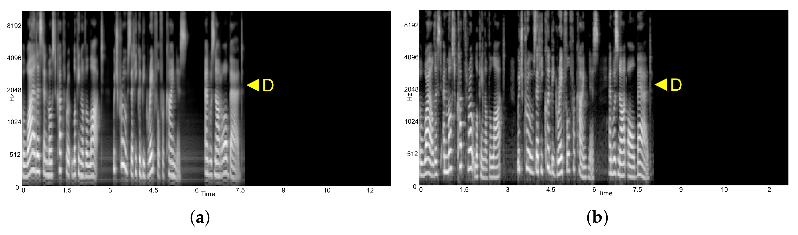
Using the corresponding transcript of LJSpeech with both a human voice and deepfake voice, a detailed comparative analysis can be conducted, which assists the user in interpretation for decision-making. As can be seen in Figure 6 and Figure 7a,d, Deep Taylor maintained highlights distinctively for each real human voice and deepfake voice at a frequency around 2 kHz, which is marked as area C. Inspecting the spectrogram in Figure 8 area D based on the assistance of the attribution score, the deepfake voice showed a flatter waveform around 2 kHz, whereas the human voice showed more variance.

5.3. Audio Interpretability

Currently, interpretability is focused on a visual method, i.e., a heatmap on a spectrogram, to interpret the model. With the visual approach, diverse characteristics of the model’s tendency, depending on XAI methods and data types, have been found. Through visual interpretation, the user can confirm what the model is focusing on. However, visual interpretation has certain limitations in intuitiveness and in assisting decision-making. Using the Griffin–Lim algorithm, the attribution scores of each model and XAI method were recomposed back to audio. For the CNN-only model, because of the tendency of XAI methods to show dependencies on energy-like formants, most of the original voice was recovered during the conversion from the attribution score. The transcript of the original voice can be recognized from the recomposed voice as well.

The attribution scores of Deep Taylor and LRP on the CNN-LSTM-based model showed less sensitivity to the energy, losing highlights on formants. Consequently, the transcript was unrecognizable on the recomposed voice. In the case of the recomposed voice of Deep Taylor and LRP on the CNN-LSTM model, because of the lack of sensitivity on formants 1, 2, and 3, the transcript of the speech was unrecognizable.

However, with the recomposed voice, visually unrecognizable characteristics, general pitch variance, and rhythm of the speech were revealed with the removal of formant dependency on the attribution score of the CNN-LSTM model. Hence, the LRP attribution score on the recomposed voice showed relatively distinct differences between the voiced and unvoiced sections.

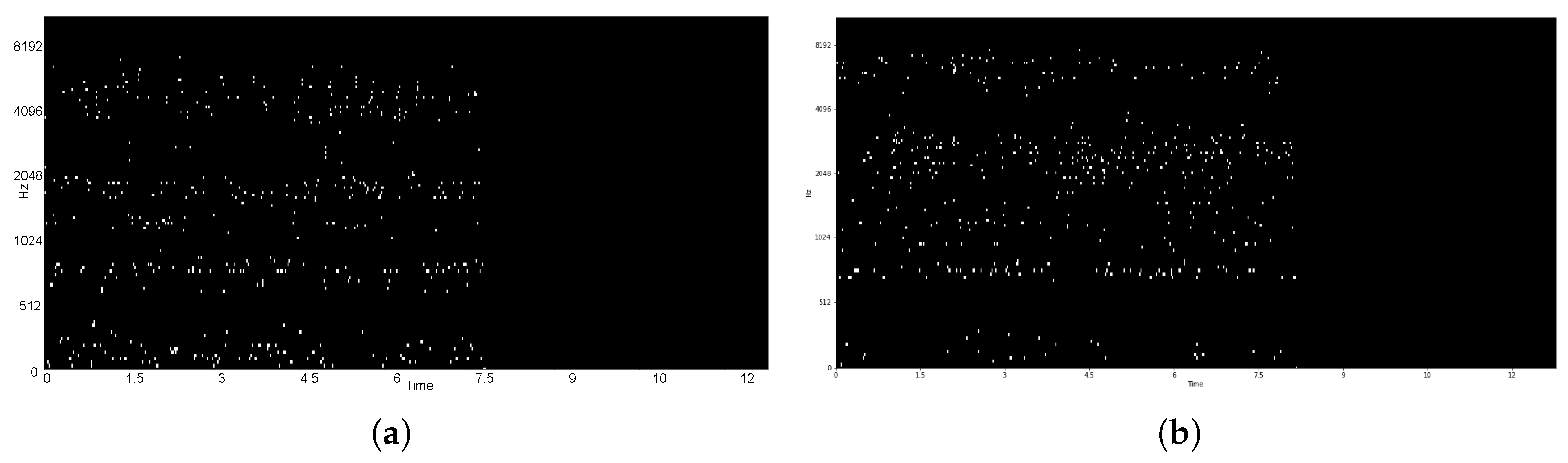
Rhythm and pitch variance differences on a Deep-Taylor-based recomposed voice can assist in distinguishing a human voice from a deepfake voice. The features showed significantly high variances in a human voice compared to the deepfake, which is presumably considered an accent, which is a feature that the generative model did not train for. Figure 9 shows the top 10% of the amplitude of the recomposed speech as a visual reference, for the comparison of pitch and rhythm variances between the deepfake and human voice.

Based on the audio interpretation, i.e., the spectrograms in Figure 8, energy distribution on frequency 2 kHz showed distensibility. The deepfake voice showed a relatively flat pattern compared to a human voice, while the human voice showed randomness. This phenomenon was assumed to be triggered by the absence of training on accents while generating training data from the LJSpeech through Tacotron TTS. This absence resulted in a flat rhythm and accent.

6. Conclusions

In this paper, we presented a general interpretation for deepfake audio detection by analyzing the attribution score patterns of several post-hoc XAI methods. Based on the characteristics of the XAI methods found in image classification, we applied them to the audio domain and attempted to interpret the characteristics at a higher level to enable non-expert cognition.

Using traditional methods used for audio-related tasks, the attribution score of the deepfake detection model was interpreted. Under a certain environment, we could find a clear distinction in formants and voiced–unvoiced speech. The experiment showed a consistent interpretation of each XAI method under various environments.

Furthermore, by recomposing the attribution score back to audio, human cognition became easier as a supplementary recognition assist. With this assist, the interpretation teardown needed to be less exclusive. With the recomposed audio, the end-user could be provided interpretation with intuitive differences in high-frequency pitch variance and a general rhythm of the speech.

Through the experiment, model interpretability on deepfake voice detection could be obtained and explained at a human cognitive level using existing XAI methods. As the current study has identified differences between model and human perception in detecting deepfake media, implementation of the marker without human recognition can be studied in the future to relieve public anxiety towards generative models creating fake media.

References

- Dolhansky, B.; Bitton, J.; Pflaum, B.; Lu, J.; Howes, R.; Wang, M.; Ferrer, C.C. The deepfake detection challenge (dfdc) dataset. arXiv 2020, arXiv:2006.07397. [Google Scholar]
- Malolan, B.; Parekh, A.; Kazi, F. Explainable deep-fake detection using visual interpretability methods. In Proceedings of the 2020 3rd International Conference on Information and Computer Technologies (ICICT), San Jose, CA, USA, 9–12 March 2020; pp. 289–293. [Google Scholar]
- Baevski, A.; Zhou, H.; Mohamed, A.; Auli, M. wav2vec 2.0: A framework for self-supervised learning of speech representations. arXiv 2020, arXiv:2006.11477. [Google Scholar]
- Dong, L.; Xu, S.; Xu, B. Speech-transformer: A no-recurrence sequence-to-sequence model for speech recognition. In Proceedings of the 2018 IEEE International Conference on Acoustics, Speech and Signal Processing (ICASSP), Calgary, AB, Canada, 15–20 April 2018; pp. 5884–5888. [Google Scholar]
- Gulati, A.; Qin, J.; Chiu, C.C.; Parmar, N.; Zhang, Y.; Yu, J.; Han, W.; Wang, S.; Zhang, Z.; Wu, Y.; et al. Conformer: Convolution-augmented transformer for speech recognition. arXiv 2020, arXiv:2005.08100. [Google Scholar]
- Kanagasundaram, A.; Vogt, R.; Dean, D.; Sridharan, S.; Mason, M. I-vector based speaker recognition on short utterances. In Proceedings of the 12th Annual Conference of the International Speech Communication Association, Florence, Italy, 27–31 August 2011; pp. 2341–2344. [Google Scholar]
- Snyder, D.; Garcia-Romero, D.; Sell, G.; Povey, D.; Khudanpur, S. X-vectors: Robust dnn embeddings for speaker recognition. In Proceedings of the 2018 IEEE International Conference on Acoustics, Speech and Signal Processing (ICASSP), Calgary, AB, Canada, 15–20 April 2018; pp. 5329–5333. [Google Scholar]
- Variani, E.; Lei, X.; McDermott, E.; Moreno, I.L.; Gonzalez-Dominguez, J. Deep neural networks for small footprint text-dependent speaker verification. In Proceedings of the 2014 IEEE International Conference on Acoustics, Speech and Signal Processing (ICASSP), Florence, Italy, 4–9 May 2014; pp. 4052–4056. [Google Scholar]
- Ito, K.; Johnson, L. The LJ Speech Dataset. 2017. Available online: https://keithito.com/LJ-Speech-Dataset/ (accessed on 15 June 2021).
- Wang, X.; Yamagishi, J.; Todisco, M.; Delgado, H.; Nautsch, A.; Evans, N.; Sahidullah, M.; Vestman, V.; Kinnunen, T.; Lee, K.A.; et al. ASVspoof 2019: A large-scale public database of synthesized, converted and replayed speech. Comput. Speech Lang. 2020, 64, 101114. [Google Scholar] [CrossRef]
- Bharadhwaj, H. Layer-wise relevance propagation for explainable deep learning based speech recognition. In Proceedings of the 2018 IEEE International Symposium on Signal Processing and Information Technology (ISSPIT), Louisville, KY, USA, 6–8 December 2018; pp. 168–174. [Google Scholar]
- Montavon, G.; Lapuschkin, S.; Binder, A.; Samek, W.; Müller, K.R. Explaining nonlinear classification decisions with deep taylor decomposition. Pattern Recognit. 2017, 65, 211–222. [Google Scholar] [CrossRef]
- Sundararajan, M.; Taly, A.; Yan, Q. Axiomatic attribution for deep networks. arXiv 2017, arXiv:1703.01365. [Google Scholar]
- Bracewell, R.N.; Bracewell, R.N. The Fourier Transform and Its Applications; McGraw-Hill: New York, NY, USA, 1986; Volume 31999. [Google Scholar]
- Meng, H.; Yan, T.; Yuan, F.; Wei, H. Speech emotion recognition from 3D log-mel spectrograms with deep learning network. IEEE Access 2019, 7, 125868–125881. [Google Scholar] [CrossRef]
- Digby, A.; Towsey, M.; Bell, B.D.; Teal, P.D. A practical comparison of manual and autonomous methods for acoustic monitoring. Methods Ecol. Evol. 2013, 4, 675–683. [Google Scholar] [CrossRef]
- Zhou, Y.; Lim, S.N. Joint Audio-Visual Deepfake Detection. In Proceedings of the IEEE/CVF International Conference on Computer Vision (ICCV), Montreal, BC, Canada, 11–17 October 2021; pp. 14800–14809. [Google Scholar]
- Becker, S.; Ackermann, M.; Lapuschkin, S.; Müller, K.R.; Samek, W. Interpreting and explaining deep neural networks for classification of audio signals. arXiv 2018, arXiv:1807.03418. [Google Scholar]
- Jung, Y.J.; Han, S.H.; Choi, H.J. Explaining CNN and RNN Using Selective Layer-Wise Relevance Propagation. IEEE Access 2021, 9, 18670–18681. [Google Scholar] [CrossRef]
- Shen, J.; Pang, R.; Weiss, R.J.; Schuster, M.; Jaitly, N.; Yang, Z.; Chen, Z.; Zhang, Y.; Wang, Y.; Skerrv-Ryan, R.; et al. Natural tts synthesis by conditioning wavenet on mel spectrogram predictions. In Proceedings of the 2018 IEEE International Conference on Acoustics, Speech and Signal Processing (ICASSP), Calgary, AB, Canada, 15–20 April 2018; pp. 4779–4783. [Google Scholar]
- Nam, W.J.; Gur, S.; Choi, J.; Wolf, L.; Lee, S.W. Relative attributing propagation: Interpreting the comparative contributions of individual units in deep neural networks. In Proceedings of the AAAI Conference on Artificial Intelligence, New York, NY, USA, 7–12 February 2020; Volume 34, pp. 2501–2508. [Google Scholar]
- Griffin, D.; Lim, J. Signal estimation from modified short-time Fourier transform. IEEE Trans. Acoust. Speech Signal Process. 1984, 32, 236–243. [Google Scholar] [CrossRef]