On the Black-Box Challenge for Fraud Detection Using Machine Learning (II): Nonlinear Analysis through Interpretable Autoencoders

Abstract

Artificial intelligence (AI) has recently intensified in the global economy due to the great competence that it has demonstrated for analysis and modeling in many disciplines. This situation is accelerating the shift towards a more automated society, where these new techniques can be consolidated as a valid tool to face the difficult challenge of credit fraud detection (CFD). However, tight regulations do not make it easy for financial entities to comply with them while using modern techniques. From a methodological perspective, autoencoders have demonstrated their effectiveness in discovering nonlinear features across several problem domains. However, autoencoders are opaque and often seen as black boxes. In this work, we propose an interpretable and agnostic methodology for CFD. This type of approach allows a double advantage: on the one hand, it can be applied together with any machine learning (ML) technique, and on the other hand, it offers the necessary traceability between inputs and outputs, hence escaping from the black-box model. We first applied the state-of-the-art feature selection technique defined in the companion paper. Second, we proposed a novel technique, based on autoencoders, capable of evaluating the relationship among input and output of a sophisticated ML model for each and every one of the samples that are submitted to the analysis, through a single transaction-level explanation (STE) approach. This technique allows each instance to be analyzed individually by applying small fluctuations of the input space and evaluating how it is triggered in the output, thereby shedding light on the underlying dynamics of the model. Based on this, an individualized transaction ranking (ITR) can be formulated, leveraging on the contributions of each feature through STE. These rankings represent a close estimate of the most important features playing a role in the decision process. The results obtained in this work were consistent with previous published papers, and showed that certain features, such as living beyond means, lack or absence of transaction trail, and car loans, have strong influence on the model outcome. Additionally, this proposal using the latent space outperformed, in terms of accuracy, our previous results, which already improved prior published papers, by 5.5% and 1.5% for the datasets under study, from a baseline of 76% and 93%. The contribution of this paper is twofold, as far as a new outperforming CFD classification model is presented, and at the same time, we developed a novel methodology, applicable across classification techniques, that allows to breach black-box models, erasingthe dependencies and, eventually, undesirable biases. We conclude that it is possible to develop an effective, individualized, unbiased, and traceable ML technique, not only to comply with regulations, but also to be able to cope with transaction-level inquiries from clients and authorities.

1. Introduction

As already stated in the companion paper [1], the rapid development of e-commerce online payment has become more and more popular, and therefore it also represents a challenge, not only to secure the transactions but also to avoid false positives in fraud detection algorithms. According to a report by The Alan Turing Institute [2], the number of transactions wrongly rejected due to suspected fraud can pose an equivalent threat to actual fraud in the industry of the financial services. Another study stated that transactions that were wrongly declined due to suspected fraud account for USD 118 billion in retail losses [3]. As a consequence, the banks are now forced to devote an increasing amount of resources to discriminate among legitimate transaction and fraud to cope with the difficult dilemma of avoiding impostors’ actions while not limiting e-commerce’s inexorable growth. However, this is not an easy task, since scammers try their best to ensure that the profiles of the transactions differ as little as possible from the real ones, trying to model extremely assimilated behavioral profiles [4]. To cope with this emerging new reality, financial institutions hire skilled expert fraud software engineers, who develop full packages of new and sophisticated strategies to pursue this purpose.

Fraud detection primitive strategies, such as expert systems, were very much related to checklists of risk factors, e.g., repeated declined transactions, multiple failed attempts to enter a credit card number, or living beyond means. However, the emergence of machine learning (ML) techniques has allowed the creation of new schemes capable of providing more adequate and precise alternatives to respond to the potential (or actual) security threats based on historical transactional records. From a mathematical perspective, credit fraud detection (CFD) could be seen and analyzed as a novelty detection problem [2]. In this direction, a possible approach could be to find lower dimensional embeddings to model the original dataset, where anomalies are expected to be detached from normal data [5].

Autoencoders have recently emerged as a resourceful deep learning family of methods for dimensionality reduction and feature extraction. According to the literature, these techniques have shown to offer improvements in accuracy, computational efficiency, and the subsequent user satisfaction in their applications [6]. Even so, one of the big challenges, and a potential barrier, for autoencoders is the lack of visibility of the underlying model in the encoding and decoding sides. Therefore, these data-driven models are frequently considered as black boxes, meaning that although inputs and outputs are known, and regardless of the good results provided in many problems, the model itself exhibits relevant limitations to show the role played by each of the features in the final outcome. That is why the authorities and regulatory bodies have shown, to date, significant reluctance to accept a generalized use of these modern techniques [7]. Although this reality becomes a clear limitation, the wide consensus among researchers and financial institutions suggests that ML still has great potential, even though a number of challenges still require special attention [8]. As an example, in the case of the United States and in order to avoid any discrimination, the features such as race, sex, or marital status, or any related one, should be very carefully applied or even not used according to existing regulations [9]. Moreover, an algorithm to lend money could be found in violation of this prohibition even if the algorithm does not directly use any of the prohibited categories, but instead it uses data that can be highly correlated with the protected categories. Lack of transparency is becoming a real challenge in fact in the European Union, as the General Data Protection Regulation adopted in 2018 gives its citizens the right to receive an explanation of decisions based on automated processing [8]. The justification for this type of regulation lies in the potential bias that the hidden stages of the model could be applying, thus leaving the individual, the regulatory body, and the risk assessment entity devoid of tools to identify any undesirable situations that finally might be reproducing [6,10]. Even more, the data used to train the ML models may not be representative for the problem [8], sometimes driving eventually to inaccurate models, with limited generalization capabilities. Having said that, and returning to regulatory restrictions, the entities understand the need for a regulation that ensures that the use of technology cannot inadvertently cause discriminatory treatment of people, but they also agree on the need for a clearer guidance from the authorities that offer a reasonable path towards the necessary and effective application of AI in this field [11]. Considering that regulatory bodies and administrative authorities will not allow financial institutions to adopt AI models without addressing the necessary description of the decision process being followed [7], a suitable way to overcome the regulatory issues and the mistrust with respect to the algorithms being used is to provide the regulators, authorities, and financial entities with supplemental environments and tools that contribute in an effectual way to the real interpretability. Therefore, we can state that decision models should be easy to understand, meaningful, and traceable. This last one means that each initial variable or feature needs to be linked to final decision score through a visible value, process, or function [7,9,12].

To accomplish this challenging goal, state-of-the-art methods in novelty detection such as autoencoders can be extremely useful, as well as a new set of strategies to offer interpretability on what was traditionally considered a black-box model. Under this perspective, the contribution of this work is a novel methodology to address the mentioned complexity. The methodology proposed in this work has a triple objective: First, to reduce the dimensionality by selecting the informative features; second, to efficiently compress and encode data to isolate fraud transactions from non-fraudulent ones; third, to propose, and eventually evaluate, novel techniques to offer a comprehensive explanatory model in CFD. To achieve this, we propose an explanation at the level of a single instance artificially generating a set of data around said instance (through random sampling and using controlled perturbations), and finally, applying a linear learning model to the distance between the instance and the sampling data. This last step represents the main difference with respect to previous applications in terms of the ability to tie input features to the outputs, thus providing the desirable interpretability. To approach the dimensionality reduction, we use the positive results included in the companion paper [1] where we applied a novel feature selection technique, the informative variable identifier (IVI) [13], which can distinguish among informative, redundant, and noisy variables or features.

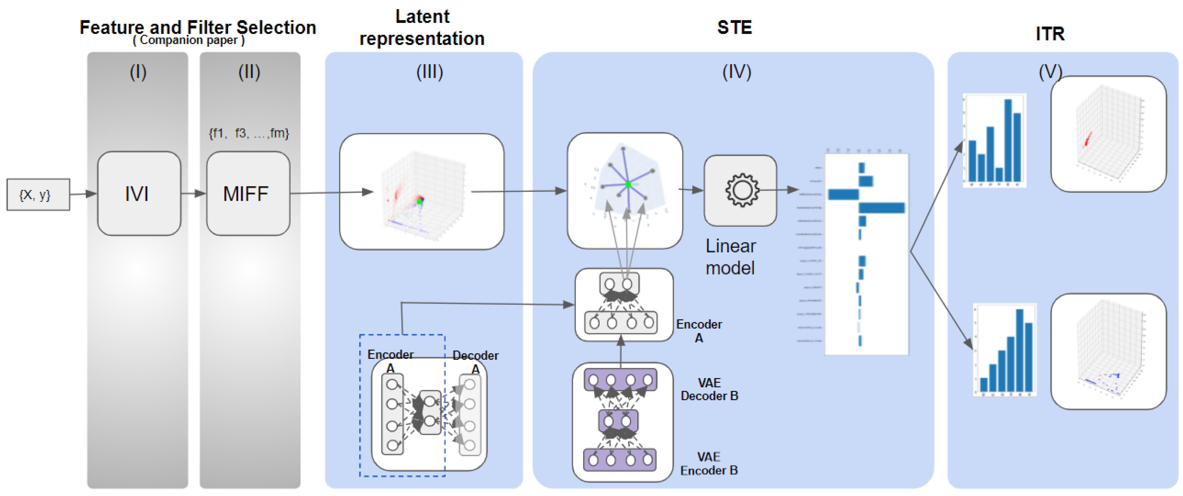
This work is organized as follows. A short review of the vast literature in the field of CFD and ML-based systems is presented in Section 2. In Section 3, a summary of new nonlinear ML algorithms used in this work is described, as well as explanatory strategies to convey an effective interpretation, as single transaction-level explanation (STE) and individual transaction rankings (ITR) are introduced and formally described. In Section 4, the different datasets are defined, and we present the qualitative and quantitative benchmarking over different datasets while maintaining the interpretability. Finally, in Section 5, discussion and observations are given, and conclusions are summarized.

2. Related Work

CFD is the process or the set of techniques followed in order to classify a transaction as fraudulent or not, in contrast to legitimate operations. This process could be understood from a methodological perspective as under the novelty detection category of data-driven problems. Nowadays, a large number of the transactions take place digitally, by means of credit cards and other electronic payment systems, increasingly challenging the fraud control systems of financial institutions worldwide. Although the fraud accounts only for 0.1% of the total transactions, the large and growing volume of the electronic market has forced the industry to devote tremendous efforts aimed to secure this new and almost indispensable way of working [14].

Among many novelty detection methods, the design of low-dimensional embeddings is becoming a relevant strategy in ML. This method suggests that once the original domain data, including anomalies and normal samples, are introduced in the model, examples are squeezed into a lower dimensional space, where these distinctive classes are expected to be separated. The projection of all samples in the new space, also known as the latent space, is referred to in the literature as a manifold or as an embedding, and it can represent a useful and illustrative plot of the dataset. In a second step, those low-dimensional embeddings are transferred back to the original space through a process called reconstruction. The training process which minimizes error or distance among samples from the original space and reconstructed space will perform the rest. If the training process concludes successfully, it is expected to yield a picture of the true intrinsic nature of the data in the latent space, without unnecessary features or noise. In other words, if the high-dimensional dataset is compressed into a limited number of new features, and it is subsequently reconstructed into the original space back again with a minimum error, then we can reckon that the features of the low-dimensional space keep all the relevant features of the initial samples. Principal component analysis (PCA) could be understood as a low complexity and linear-type example of this set of techniques, where the new features are ranked by variance [5]. In the same direction and with the advent of deep learning, a new group of techniques is being opened. 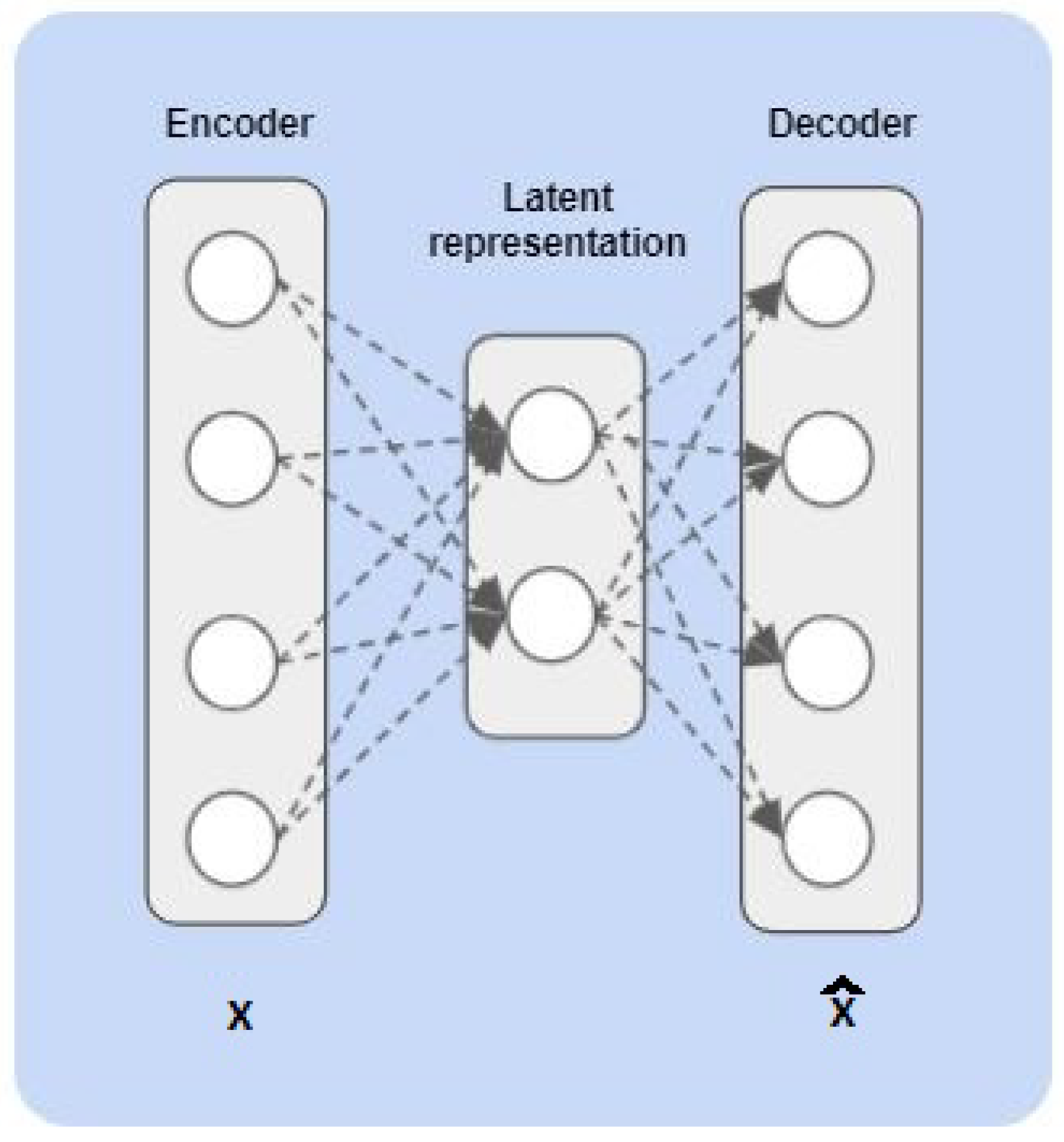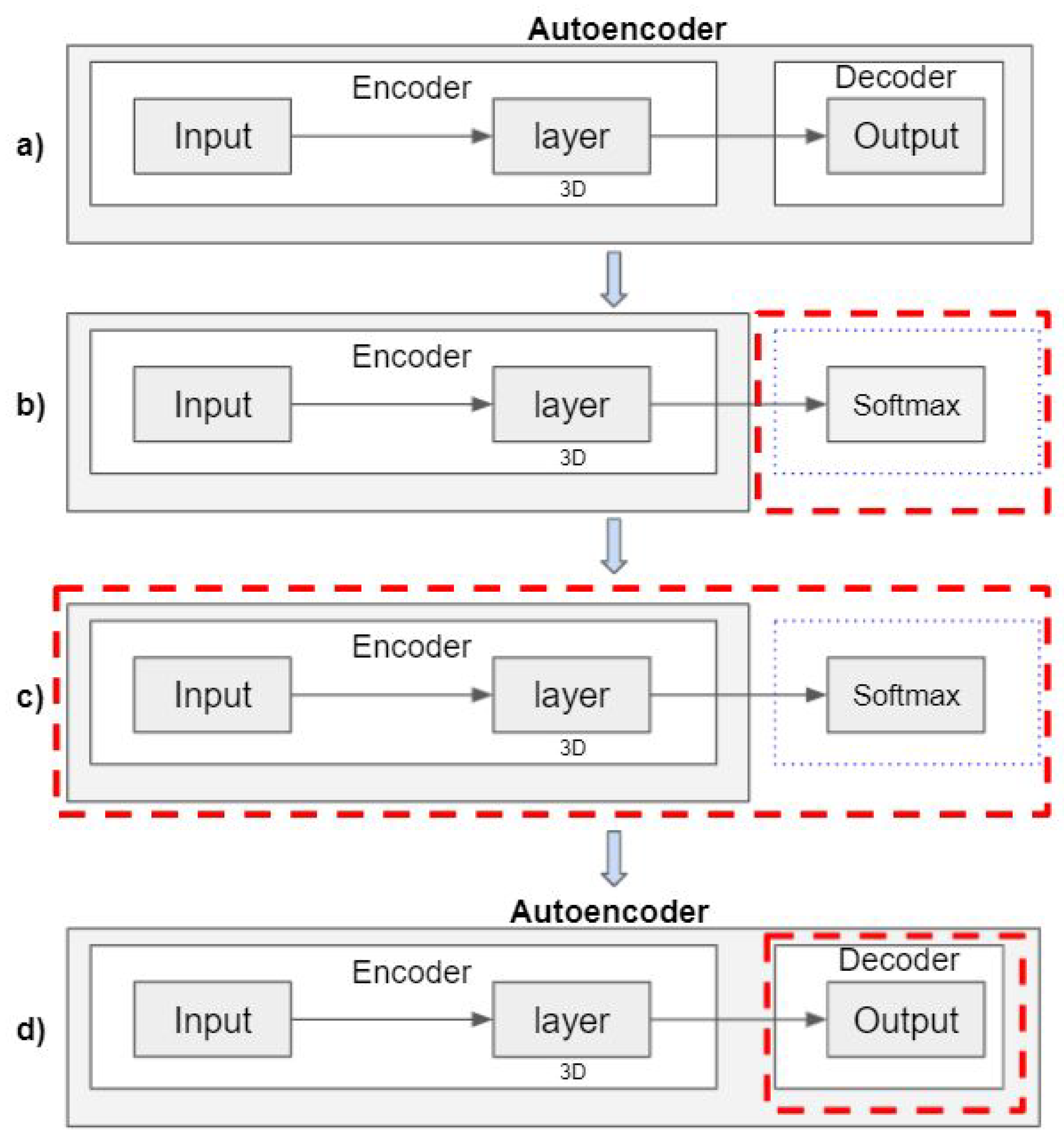On the one hand, specialized embedding approaches for natural language processing have emerged [15,16,17,18,19,20,21], and on the other hand, autoencoders are becoming among the most promising approaches for feature extraction and dimensionality reduction [22]. An autoencoder [23,24] is a multiple layer neural network that compresses the high-dimensional data into a low-dimensional latent representation (encoder), combined with a later expansion to the original space (decoder). As a result, autoencoders are able to discover a lower-level representation of a higher dimensional data space [25]. Considering that the autoencoder training processes tend to minimize the distance among original input space and the regenerated space through the two-stage encode–decode methodology, it could be understood that the existing low-dimensional (or latent) space summarizes the essence of the actual data, as the decoder is capable of expanding those low-dimensional data to the original dimension. In other words, we could make a case saying that the hidden layers of the encoder are able to extract the features that better represent the actual data with the current dimensional constraint. This procedure, although considered a black-box method, shows good performance in the CFD field according to literature [26,27].

As we introduced in Section 1, financial services and, more specifically, CFD are highly regulated areas, with almost no room for black boxes, for models which are difficult to understand, or for architectures without adequate transparency in their use of the data. All this leads to the need for interpretability as a crucial element when it comes to breaking the barriers of lack of transparency in traditional ML developments. A good number of papers have delved into this issue, pointing out how the increase in complexity works against transparency [11], how regulations of the United States and Europe tighten their vigilance on the correct use of the features [8], and how the absence of these criteria can lead to unacceptable bias for the application of ML techniques [11]. An important challenge in ML is interpretability, which refers to the interpretation of the reasons behind the model decision in a way that humans can understand, that is, human beings would be able to have full understanding about the model logic [7]. However, in the field of financial services, there is no shortage of entities that point out the difficulty of making use of the powerful ML tools for fraud detection and simultaneously complying with the increasingly restrictive regulatory requirements. This does not mean that regulation is seen as an unjustified barrier to ML deployment, although some entities do emphasize the need for a certain guidance on how to take it into consideration in the context of the CFD architectures [11]. To cope with it, and according to existing literature, financial institutions rely on using simple interpretable models, such as decision trees [28] or linear models [12]. These kinds of models are easy to understand, and their predictions are straightforwardly explained. In the case of decision trees, for instance, interpretation can be followed through the branches, and in the case of linear models, interpretations depend on the weights for each feature in the model. In other direction, new strategies are currently focused on local surrogate models and specifically on local interpretable model-agnostic explanations (LIME) [29]. In this last method, the authors, instead of training a global surrogate model, use local surrogates to approximate predictions of the underlying black-box model. This is performed by modifying a single instance by tweaking the feature values and observing the impact on the output. This procedure is reproduced at a local level, and it effectively generates a valid surrogate model for a tight environment of the local instances. By doing so, LIME generates an interpretable, agnostic, and locally meaningful alternative to the original black-box data model. Finally, other studies have elaborated on the binomial interpretability vs. accuracy. In [30], the authors elaborate on the trade-off among the cost of interpretability vs. the predictive capabilities, concluding that currently, in financial services, interpretability is even more important than accuracy, as it is mandatory to comply with regulations.

It is clear, according to the literature [31,32], that dimensionality reduction is more than needed in order to be able to classify and identify anomalies in a daily growing dataset environment. It is quite frequent in the artificial intelligence business to think that the larger the number of features, the more possibilities we must articulate, as a feasible model that fits the latent reality. This often means a continuous exponential increase in features, and consequently, the quality of the data required to process ML algorithms gradually decreases. This effect has long been known as the curse of dimensionality [33,34]. In fact, higher dimensions lead to the existence of redundant information, noisy samples, and irrelevant information, which may cause overfitting of the model and may increase the error rate of the learning algorithms. To handle these problems, direct and previous dimensionality reduction can be applied. The classical approach to the previous issues is the use of feature selection (FS) techniques. FS is used to clean up and pre-evaluate the possible contribution of the features in terms of valid information by removing noisy, redundant, and irrelevant data [32]. FS methods can improve accuracy, efficiency, effectiveness, and even interpretability to the learning process. For this reason, a large number of automatic FS methods have been developed in the past. In FS, a subset of features is selected from the original set, based on the evaluation of the actual intrinsic information of each feature, namely, the redundancy and the relevance [31]. During this process, features are classified into the following four groups according to their eventual effective information: (1) noisy and irrelevant; (2) redundant and weakly relevant; (3) weakly relevant and non-redundant; (4) strongly relevant. Popular approaches to carry this out are filter methods, wrapper methods, and embedded methods. Filter methods analyze the usefulness of each single feature through the use of relevance techniques, mainly from hypothesis tests or estimates of mutual information [35]. Wrapper methods solve ML problems to assess the relevance of each feature in the input space [36]. Finally, embedded methods, such as recursive feature elimination (RFE) [37], aim to increase their efficiency by combining the FS procedure with training a subsequent learning machine. Many of these embedded methods impose a regularization on the solution. A special mention is required for a recently proposed novel feature selection method, called IVI [1,13]. This technique is capable of isolating informative, redundant, and noisy features automatically. One of its main characteristics is being able to transform the distribution of the input variable space into a coefficient feature space by using existing linear classifiers or efficient weight generators. At this point, it is necessary to mention that a large number of feature selection methods have been published in the literature, with uneven results in their application in different disciplines. It is not the object of this article to carry out a detailed analysis of each and every one of these techniques, but for the reader’s convenience and with the intention of offering a summary of the different typologies of published methods, hereafter in

Table 1. Summary table of feature selection methods (FS) present in the literature according to the basic techniques used [32,38].

FS Method	Summary
Filter methods	They use statistical techniques to evaluate the relationships among characteristics (i.e., Pearson’s correlation, chi-square) [35].
Wrapper methods	They are based on the inferences that we draw from a previous model, and we decide to add or remove features from our subset (i.e., forward feature selection and backward feature selection) [36].
Embedded methods	They combine the qualities of filter and wrapper methods. They are implemented by algorithms that have their own built-in feature selection methods (i.e., RFE) [37].
IVI	It is capable of identifying the informative variables and their relationships. It transforms the input-variable space distribution into a coefficient-feature space [1,13].

a schematic summary is presented for the different types of techniques as published in various reviews [32,38], including a new category for the informative variable identifier (IVI) that we included in this paper [13].

3. Materials and Methods

This section is structured as follows. First, all datasets are introduced and described. Second, a brief reference of ML algorithms used in this work is presented. Third, the FS technique applied here, namely, the IVI algorithm, is described as a novel and key strategy to pursue interpretability. Next, the proposed methodology developed in this work is shown, and finally, the explanatory strategies to effective guide interpretability are presented.

3.1. Datasets

One of the main problems in CFD literature is the lack of information due to the confidentiality of the data such that it is not easy to find representative, informative, and open datasets. For this reason, we have first used a synthetic dataset to validate our proposal [1], thus paving the way for a later analysis over real datasets.

Synthetic Dataset. The first dataset introduces a synthetic linear classification problem with a binary output variable, and it was developed in the original proposal of the IVI algorithm [13] with 485 input features. For this work, and for reasons of representability and execution time, we have used a subset of features while keeping the feature names. This subset was selected with the first features of each group. The dataset used for this work includes a set of 23 input features distributed as follows: 11 input features drawn from a normal distribution, 5 of them are used to linearly generate a binary output variable, specifically $f0,f1,f2,f3$, and $f4$. Therefore, these five features will be informative for the problem. A set of another 12 features are randomly created with no relation to the previous ones and so they could be considered as noisy and non-informative features. Additionally, a new group of 6 features are computed as redundant with the informative input features.

German Credit Dataset. This set is known as German Credit Fraud (Stattog) [39], and it contains real data used to evaluate credit applications in Germany. We used a version of this dataset that was produced by the Strathclyde University. The German Credit Dataset contains information on 1000 loan applicants. Each applicant is described by a set of 20 different features with a binary output variable. Among these 20 features, 17 of them are categorical while three are continuous. There are no missing values. To facilitate FS and in order to train the models, the values of the three continuous attributes were normalized, and for the discrete features they were converted to one hot encoding. After these preprocessing stages, the final dataset was 61-dimensional. Detailed information for each feature can be found in [39] and there is a short description in

Table 2. Summary table of features in German Credit Dataset.

Feature	Description
Status	Status of existing checking account
Duration	Credit duration in months
Credit history	Credit application history
Purpose	Credit propose
Amount	Credit amount
Savings	Savings account/bonds
Employment	Years in last job
Personal status	Personal status and sex
Other parties	Other debtors/guarantors
Property magnitude	Real estate owned or life insurance
Age	Age in years
Housing	Rent or own
Number of credits	Number of existing credits at this bank
Job	Current job
Telephone	Proprietary telephone
Foreign worker	Is foreign worker
Other payment plans	Other installment plans
Credit balance	Average credit balance
Location	Location
Overdraft	Historical overdraft

.

PaySim Dataset. PaySim simulates mobile money transactions based on a sample of real transactions extracted from one month of financial logs from a mobile money service implemented in an African country [40]. The original logs were provided by a multinational company, who is the provider of the mobile financial service which is currently running in more than 14 countries all around the world. PaySim covers five of the most important transaction types: cash-in, cash-out, debit, payment, and transfer. The PaySim dataset contains information on 6,362,620 transactions. Each applicant is described by a set of 11 different features. For performance reasons, in this work we have selected a subset transaction with 25,867 transactions selected randomly maintaining a distribution with 80% non-fraud transactions and 20% fraud transactions. Detailed information for each feature can be found in [40] and there is a short description in

Table 3. Summary table of features in PaySim Dataset.

Feature	Description
Step	Maps a unit of time in the real world. In this case 1 step is 1 h of time
Type	Cash-in, cash-out, debit, payment, and transfer.
Amount	Amount of the transaction in local currency.
NameOrig	Customer who started the transaction.
OldbalanceOrg	Initial balance before the transaction.
NewbalanceOrig	New balance after the transaction.
NameDest	Customer who is the recipient of the transaction.
OldbalanceDest	Initial balance recipient before the transaction.
NewbalanceDest	New balance recipient after the transaction.
IsFraud	This is the transactions made by the fraudulent agents inside the simulation.
IsFlaggedFraud	The business model aims to control massive transfers from one account to another and flags illegal attempts. An illegal attempt in this dataset is an attempt to transfer more than 200,000 in a single transaction.

.

3.2. ML Algorithms

As we have introduced, the origins of the CFD systems date back to around the late 1990s. Initially, these systems were almost always based on experts’ rules, and with the passage of time until now, ML systems have been developed to enhance the accuracy [2,4,6,41]. In this respect, linear classifiers based on ML are very useful in CFD because they can be seen as a transformation from the space of the input features to weightings to each of these features in the decision process [13]. From this point of view, those weights summarize the contribution of each feature in the decision process, and they can be used to interpret the models. A detailed analysis of learning methods has been proposed with the efforts presented in the companion paper [1]. In the following lines, we first introduce the notation used throughout the paper. Let $\mathbf{X}\in {\mathbb{R}}^{N\times L}$ be the input data matrix, containing the input set of vectors in rows, with N observations of L features, where ${\mathbf{x}}_n$ is a vector with L features for $n=1,\dots ,N$. We consider a classification problem with a binary output variable $\mathbf{y}\in {\mathbb{R}}^N$, grouped in the observations in a vector such that ${\mathbf{y}}_n\in \left\{-1,+1\right\}$ for $n=1,\dots ,N$. Second, we present the summary of new nonlinear ML algorithms, such as the autoencoders, which we use in the rest of the article.

An autoencoder [42] is a specific type of neural network, which is designed to encode the input into a compressed and meaningful representation, and then to decode it back such that the reconstructed input is as similar as possible to the original one. The potential of autoencoders is to compress high-dimensional data into latent representations, that is why they are defined as two parts: an encoder and a decoder, where the encoder learns to map the high-dimensional input space to a latent vector space, and the decoder maps the latent vector space to the original uncompressed input space. Overall, the output data matrix $\hat{\mathbf{X}}$ is the result of reconstructing the original input data matrix $\mathbf{X}$. We can see the architecture of a basic autoencoder in Figure 1.

The problem, as formally defined in [43], consists of the transformation from an L dimensional domain or $R^L$ toward a lower dimensional space, $R^P$, recalled as encoder, followed by a second transformation from the latent space $R^P$ to the reconstructed space $R^L$, recalled as decoder. This problem is defined to minimize the reconstruction error after the encoding–decoding procedure.

Variational Autoencoders

Over time, autoencoder models have emerged with different approaches, one of which are the variational autoencoders (VAEs) [43]. VAE are autoencoders whose encoding distribution is regularized during their training in order to ensure that its latent space has good properties, allowing us to generate new samples that are consistent with actual data. Formally, VAEs are generative models that attempt to describe how the data might be generated through a probabilistic distribution. Specifically, given an observed dataset $\mathbf{X}$, we assume a generative model for each datum ${\mathbf{x}}_i$ conditioned to an unobserved random latent variable ${\mathbf{z}}_i$, where $\mathit{\theta }$ are the parameters governing the generative distribution. This generative model is also equivalent to a probabilistic decoder. Symmetrically, we assume an approximate posterior distribution over the latent variable ${\mathbf{z}}_i$ given a datum ${\mathbf{x}}_i$ denoted by recognition, which is equivalent to a probabilistic encoder which is governed by parameters $\mathit{\varphi }$. Finally, we assume a prior distribution for the latent variables ${\mathbf{z}}_i$ denoted by ${\mathbf{p}}_0\left({\mathbf{z}}_i\right)$. The observed latent variables ${\mathbf{z}}_i$ can be interpreted as a code given by the recognition model ${\mathbf{q}}_{\mathit{\varphi }}\left(\mathbf{z}\right|\left|\mathbf{x}\right)$. The marginal log-likelihood is expressed as a sum over the individual data points as expressed next,

$$\begin{array}{c}\hfill log{\mathbf{p}}_0\left({\mathbf{x}}_i\right)=D_{KL}\left(q_{\mathit{\varphi }}\left(\mathbf{z}|{\mathbf{x}}_i\right)\left|\right|({\mathbf{p}}_0\left(\mathbf{z}|{\mathbf{x}}_i\right)\right)+\mathit{\varphi }\left(\mathit{\theta },\mathit{\varphi };{\mathbf{x}}_i\right)\end{array}$$

(1)

where the first term is the Kullback–Leibler divergence of the approximate recognition model from the true posterior and the second term is called the variational lower bound on the marginal likelihood, defined as expressed next:

$$\begin{array}{c}\hfill \mathit{\varphi }\left(\mathit{\theta },\mathit{\varphi };{\mathbf{x}}_i\right)\doteq {\mathbf{E}}_{{\mathbf{q}}_{\mathit{\varphi }}\left(\mathbf{z}|{\mathbf{x}}_i\right)}\left[-log{\mathbf{q}}_{\mathit{\varphi }}\left(\mathbf{z}|\mathbf{x}\right)+log({\mathbf{p}}_{\mathit{\theta }}\left(\mathbf{z},\mathbf{x}\right)\right]\end{array}$$

(2)

Variational inference follows by maximizing $\mathit{\varphi }\left(\mathit{\theta },\mathit{\varphi };{\mathbf{x}}_i\right)$ for all data points with respect to $\mathit{\theta }$ and $\mathit{\varphi }$.

With the intensive use of autoencoders, new techniques have been developed and techniques commonly used in other algorithms have been adapted to improve their performance, one of which is known as fine-tuning. The goal of fine-tuning is to adjust the weights of the trained model from the final phase to improve the prediction outcome. This procedure, based on the concept of transfer learning [44], includes the step of pretraining neural networks with a generative objective followed by additional training procedures with a discriminative objective on the same dataset [45], but some other studies follow the process of reusing weight values from large datasets as initialization in applications with limited access to labeled data [46]. Let $\mathbf{X}\in {\mathbf{R}}^{N\times L}$ be the input data matrix, containing the input set of vectors in rows, with N observations of L features. We consider latent space output variable $\mathbf{Y}\in {\mathbf{R}}^{P\times N}$, with P being the size of the reduction feature space or latent space. The algorithm is summarized as shown in Algorithm 1, where an autoencoder is fitted to obtain the weights, after which the encoder weights are frozen and the softmax layer is added for readjustment.

Algorithm 1 Fine-tuning.
Require: Training set $\mathbf{X}$ and result class $\mathbf{Y}$,
1:	Initialize the autoencoder $AE=\left\{\right\}$.
2:	Fit AE. $AE\leftarrow AE.fit\left(\mathbf{X}\right)$
3:	Freeze all the weights
4:	Separate AE in encoder ($enc$) and decoder ($dec$)
5:	Add Softmax layer to $enc$
	$en{c}^{\prime }\leftarrow enc+softmaxlayer$
6:	Fit $en{c}^{\prime }$ all layer’s weight freeze except softmax layer
	$en{c}^{\prime }\leftarrow en{c}^{\prime }.fit(\mathbf{X},\mathbf{Y})$
7:	Fit enc’ with unfreeze layer
	$en{c}^{\prime }\leftarrow en{c}^{\prime }.fit(\mathbf{X},\mathbf{Y})$

3.3. Informative Variable Identifier

In our proposal, we use a recently proposed feature selection method, called IVI [13], which is capable of classifying the features according to their contribution to the selected method. Mathematically, IVI methodology is based on the statistical distribution of the weights of each feature across different ML using a particular resampling technique, such as bootstrap. The joint statistical distribution of the weights of every input feature is used to define the features itself, and thus to classify each of them as informative, redundant, noisy, or not informative. Form a conceptual standpoint, we could state that it transforms the input-feature space distribution into a coefficient-feature space using existing linear classifiers or a more efficient weight generator. IVI selects the informative features and then it passes them to some linear or nonlinear classifier. Experiments have shown that IVI can outperform state-of-the-art algorithms in terms of feature identification capabilities, and even in classification performance when subsequent classifiers are used. A detailed analysis and the results obtained for IVI algorithm are presented in the companion paper [1].

3.4. Kendall Rank Correlation Coefficient

In order to evaluate the similarity between different transactions, we have used the Kendall rank correlation coefficient. Kendall rank correlation coefficient is a statistic used to measure the ordinal association between two measured quantities. Let $({\mathbf{a}}_1,{\mathbf{b}}_1),\dots ,({\mathbf{a}}_n,{\mathbf{b}}_n)$ be a set of observations of the joint random variables $\mathbf{A}$ and $\mathbf{B}$, such that all the values of $\left({\mathbf{a}}_i\right)$ and $\left({\mathbf{b}}_i\right)$ are unique. Any pair of observations $({\mathbf{a}}_i,{\mathbf{b}}_i)$ and $({\mathbf{a}}_j,{\mathbf{b}}_j)$, where $i<j$, are said to be concordant if the sort order of $({\mathbf{a}}_i,{\mathbf{a}}_j)$ and $({\mathbf{b}}_i,{\mathbf{b}}_j)$ agrees: that is, if either both $({\mathbf{a}}_i>{\mathbf{a}}_j)$ and $({\mathbf{b}}_i>{\mathbf{b}}_j)$ holds or both $({\mathbf{a}}_i<{\mathbf{a}}_j)$ and $({\mathbf{b}}_i<{\mathbf{b}}_j)$, otherwise they are said to be discordant. The Kendall $\tau$ coefficient is defined as

$$\tau =\frac{n_c-n_d}{\left(\genfrac{}{}{0pt}{}{n}{2}\right)}$$

(3)

where the $n_c$ is the number of concordant pairs, $n_d$ is the number of discordant pairs, and $\left(\genfrac{}{}{0pt}{}{n}{2}\right)$ is the total number of pair combinations. In Kendall rank correlation coefficient, the denominator is the total number of pair combinations, so the coefficient must be in the range −1 ≤ $\tau$ ≤ 1. If the agreement between the two rankings is perfect (i.e., the two rankings are the same), the coefficient has value 1. If the disagreement between the two rankings is perfect (i.e., one ranking is the reverse of the other), the coefficient has value −1. If $\mathbf{a}$ and y are independent, then we would expect the coefficient to be approximately zero.

3.5. Interpretability Methodology

This section briefly describes the four stages and five steps of the proposed methodology for the interpretability implementation. In Figure 2, we graphically depict the proposed architecture of the process. This methodology is sequentially described step by step, as follows.

• Step 1: IVI feature selection. Common informative features are extracted with the IVI algorithm.
• Step 2: Application of the MIFF filter [1].
• Step 3: Latent representation. Compress high-dimensional to a latent space in order to isolate fraud transactions.
• Step 4: STE interpretability. Feature weight evaluation for individual transactions.
• Step 5: Clustering through ITR.

Figure 2. Methodology applied to formulate interpretability. The five steps are schematically depicted here, namely: (I) selection of variables using IVI; (II) filtering of variables through MIFF (maximally informative feature filter); (III) latent space evaluation; (IV) STE modeling; and (V) ITR characterization.

Figure 2. Methodology applied to formulate interpretability. The five steps are schematically depicted here, namely: (I) selection of variables using IVI; (II) filtering of variables through MIFF (maximally informative feature filter); (III) latent space evaluation; (IV) STE modeling; and (V) ITR characterization.

For the first step of our methodology, we focused on FS. To achieve this, we applied a recently proposed FS technique called IVI [13], capable of identifying the informative, redundant, and noisy features. The IVI algorithm introduced in the original work was implemented with CME as a weight generation method designed to be competitive with the standard linear algorithms. In our methodology, we expanded the weight generator using different classification algorithms, SVM, LDA, LR, and GB (see the companion paper [1]).

It is common for FS to fall into two biases, on the one hand due to biases in the training data and on the other hand the biases are due to the intrinsic characteristics in the ML algorithms used. In this sense, the second step of our methodology focused on feature selection extension, reducing the bias and obtaining a global view of the problem. Using the IVI algorithm, we resampled the data to train ML algorithms, and in this setting, we minimized the training data bias. In the case of the bias in other ML algorithms, we used and combined different ML algorithms, aiming to discover which of these features were truly informative in all cases. For that purpose, the features needed to be subjected to a filtration process, at the end of which only the features that appeared as consistent were included in our model. In the companion paper [1], we had established two kinds of filters over the relevant features extracted by using IVI and leaving aside the redundant and noisy features: maximallyinformative features filter (MIFF) and the recurrent features filter (RFF). In this work, we focused on MIFF because we obtained the best result using this filter in the companion paper. The MIFF filter consists of selecting those features that at least have been retrieved in two of the ML algorithms used. This filter is less restrictive and provides moderate feature reduction compared with the RFF. In contrast, this filter is able to identify relationships among features achieving higher prediction accuracy.

3.6. Latent Representation

Latent space refers to a latent multi-dimensional space that contains feature values that we cannot interpret straightforwardly, but which encodes a meaningful internal representation of externally observed events, that is, it is simply a representation of compressed data in which similar data points in the latent space are also closer together in the input space. In our methodology, we built an autoencoder with an encoder and a decoder stage, where the encoder compresses the real space into a latent space in 3D for visual representative reasons. With this in mind, the autoencoder was built with a first layer with the number of cells being the number of features selected in the IVI method with the MIFF filter. The second layer has three cells (to achieve 3D representations), and finally the third layer is the reconstruction with latent space to the input space again. As it can be appreciated, the encoder is built with the first and second layers, and the decoder corresponds with the third layer. The activation functions between layers used were rectified linear units. Once we have defined the autoencoder architecture, we fit the autoencoder with the training dataset and the results for the stacked neural network can be improved by performing back propagation on the whole multilayer network. This process is often referred to as fine tuning. In this way, and to obtain a higher dispersion in the latent space, we applied a fine-tuning by adding a last softmax layer to the encoder and we fit again while freezing the encoder layers and only allowing the gradient to backpropagate through the softmax layer. We should recall at this point that the compression process runs from the initial domain of each dataset defined in Section 3.2 (of 23, 61, and 14 variables) to a latent space of only three dimensions. For a better understanding, Figure 3 represents an overview of the fine-tuning process.

3.7. Interpretability

This section describes how to achieve interpretability over the decision process. First, problem formulation is defined. Second, we introduce the transaction-based interpretability, by developing a single transaction-level explanation strategy (STE). Third, we present the details of the individual transaction rankings (ITR) algorithm, which allows us to sort features by significance. Fourth, we explain how to build global profiles based on Kendall correlation between ITR.

3.7.1. Problem Formulation

The following lines describe the credit fraud detection interpretation system (CFDIS).

Notation 1.

Let $CFDIS$ = $\langle \mathbf{T},\mathbf{F},\mathbf{C}\rangle$ be an interpretability system for CFD, where:

• $\mathbf{T}$ = $\{{\mathbf{t}}_1,\dots ,{\mathbf{t}}_n\}$ is the set of transactions participating to the system;
• $\mathbf{F}$ = $\{{\mathbf{f}}_1,\dots ,{\mathbf{f}}_m\}$ is the set of relevant features in a transaction;
• $\mathbf{C}$ = $\{{\mathbf{c}}_1,\dots ,{\mathbf{c}}_g\}$ is the set of classes in a CFD (fraud, non-fraud).

Thus, we formally define a transaction ${\mathbf{T}}_{ij}\in \mathbf{T}$ as ${\mathbf{T}}_{ij}$ = $\langle {\mathbf{t}}_i,{\mathbf{c}}_j,{\mathbf{W}}_{ij},\mathbf{F}\rangle$ where the transaction ${\mathbf{t}}_i$ is classified as ${\mathbf{c}}_j$ and its interpretability is based on the numerical weights ${\mathbf{W}}_{ij}$ for all features in $\mathbf{F}$. Typically, ${\mathbf{c}}_j$ is defined as the classes for fraud or non-fraud, assuming that they are known. We define a ranking function ≻ as the ordering of a subset of features according to their contribution to the decision process. Taking into consideration this definition, we make the following assumption:

Assumption 1.

Each transaction ${\mathbf{t}}_i\in \mathbf{T}$ has a set of ordered features in the decision process, denoted by ${\mathit{\rho }}_i=({\mathbf{F}}^i,{\succ }_{O_i})$, with ${\mathbf{F}}^i\subseteq \mathbf{F}$ and representing its features. This means that the transaction $t_i$ has a partial ordering of a subset of features ${\mathbf{F}}^i\subseteq \mathbf{F}$ according to a certain ordering function ${\succ }_{O_i}$, such that ${\succ }_{O_i}:{\mathbf{F}}^i\to \mathbf{R}$ allows the transaction $t_i$ to assign a value to a certain feature in ${\mathbf{F}}^i$, representing its weight in the decision process, regarding this particular transaction.

Example 1.

For instance, let${\mathbf{F}}^1=\{$living beyond means, lack or absence of transaction trail, car loans} be the set of features, which are made up of transaction${\mathbf{t}}_1$’s informative features in the decision process. Transaction${\mathbf{t}}_1$runs its ordering function${\succ }_{O_i}$, obtaining the weight${\mathbf{W}}_{ij}$:

• ${\succ }_{O_i}(\mathit{Living} \mathit{beyond} \mathit{means})=4.9$.
• ${\succ }_{O_i}(\mathit{Lack} \mathit{or} \mathit{absence} \mathit{of} \mathit{transaction} \mathit{trail})=4.7$.
• ${\succ }_{O_i}(\mathit{Car} \mathit{loans})=5.2$.

Then, the most representative features for${\mathbf{t}}_1$in the decision process are${\mathit{\rho }}_1=(\mathit{car} \mathit{loans}\succ \mathit{living} \mathit{beyond} \mathit{means}\succ \mathit{Lack} \mathit{or} \mathit{absence} \mathit{of} \mathit{transaction} \mathit{trail})$.

Therefore, if in a transaction the weight of feature 1 is higher than the weight of feature 2, we can infer that the decision process is being more influenced by feature 1.

Definition 1.

Using the aforementioned notation, the problem that we tackle in this work is defined as follows:

1. 

An interpretability system for CFD is represented by $CFDIS=\langle \mathbf{T},\mathbf{F},\mathbf{C}\rangle$;

2. 

A set $\left\{{\mathit{\rho }}_i\right\}$ of internal ordered weights $W_{ij}$ for each feature $\mathbf{F}$;

3. 

A set $\left\{{\mathbf{T}}^i\subseteq \mathbf{T}\right\}$ of transactions where a subset ${\mathbf{F}}^i\subseteq \mathbf{F}$ of features, belonging to ${\mathit{\rho }}_i$, are the features more representative for the decision process.

The problem is finding how to build a set describing the contribution of the features from the set of features $\mathbf{F}$ given by such $\mathbf{T}$.

Our proposal 1. As a solution to the aforementioned problem, we propose to couple the CFDIS with a mechanism that is able to evaluate the weights for each feature and for each transaction in the latent space. For that purpose, we build a VAE, as expressed in Equations (1) and (2), to obtain the latent space representation of the transaction that we want to interpret, and we generate a custom dataset with random samples using perturbations around the instance. To achieve this, we propose an STE with this custom dataset with artificial samples around the instance. These perturbations in the latent space are weighted according to their proximity to the instance of interest using a decision function. Once we have built the ITR for the more significant features, we repeat this process for all the transactions building a global ranking. However, our approach focuses on building individual rankings, which we consider has an enormous potential, as it allows us to discover the most significant features of the decision process.

3.7.2. STE Discovers the Feature Weights

As an introductory and illustrative synthesis, we can say that our STE analysis implements and validates a linear surrogate model, which validly approximates the behavior of complex black-box models for each of the samples under study. Accordingly, the weights of the aforementioned linear model could be considered as the summarized contributions of the complex and black-box model under evaluation, for each individually assessed instance.

Bearing this underlying global rationale in mind, we can describe the detailed process followed in the implementation. We start by using the selected and filtered features previously described earlier using the IVI algorithm and the MIFF filter. We implement the encoder by applying a fine-tuning technique that better encapsulates the relevant information of the input space in a 3D latent space. Once this encoder is built, a variational autoencoder will allow us to generate new surrogate and viable input samples compatible with the existing reality. Then, by using the realistic projected samples that are close enough according to a certain score distance in the latent space, a linear regression model is implemented. This linear model will be considered as the surrogate model that best matches the complex black-box model (an autoencoder model in our case) for such set of samples. Therefore, the weights of such linear model can be quantitatively used as the local single instance contribution of the aforementioned black-box model. The detailed process being followed is described in Algorithm 2, where a VAE is fitted to obtain random samples in the latent space around the transaction that we want to interpret. With these samples, we will calculate the score difference in the latent space with respect to the transaction that we want to interpret using a classifier. These score differences in the latent space are used to obtain weightings to each of the input features in the decision process by means of a linear model.

Algorithm 2 Interpretability. STE algorithm
Require: Training set in real space is $\mathbf{X}$, ${\mathbf{I}}_n$ is the transaction to interpret, encoder $enc$, number of resamples d, and number of bootstraps resamples s.
1:	Split the set $\mathbf{X}$ into two subsets, ${\mathbf{X}}_{train}$ with ${\mathbf{Y}}_{train}$ and ${\mathbf{X}}_{tes{t}_i}$ with ${\mathbf{Y}}_{tes{t}_i}$, and number of bootstraps resamples s.
2:	Initialize the $VAE=${ }.
3:	Fit VAE. $VAE\leftarrow VAE.fit\left({\mathbf{X}}_{train}\right)$.
4:	Generate realistic synthetic data. $X^{\prime }\leftarrow VAE.predict\left({\mathbf{X}}_{test}\right)$.
5:	Execute encoder to obtain the position in the latent space for instance ${\mathbf{I}}_n$.
	$I{n}_{LS}=enc.predict\left({\mathbf{I}}_n\right)$.
6:	Execute encoder to obtain the position in the latent space for ${\mathbf{X}}_{train}$.
	$X_{trai{n}_{LS}}=enc.predict\left({\mathbf{X}}_{train}\right)$.
7:	Fit a classification model in the latent space $CM$.
	$CM\leftarrow CM.fit({\mathbf{X}}_{trai{n}_{LS}},{\mathbf{Y}}_{train})$.
8:	Execute encoder to obtain the position in the latent space for realistic synthetic data $X^{\prime }$.
	$Si{n}_{L{S}_i}=enc.predict\left({\mathbf{X}}_i^{\prime }\right)$ with $i=1,\dots ,d$.
9:	Calculate score variation in the latent space.
	$Y_{scor{e}_i}=(CM.score\left(Si{n}_{L{S}_i}\right)-CM.score\left(I{n}_{LS}\right))$ with $i=1,\dots ,d$.
10:	for b← 1 to s do
11:		Generate a random subset of realistic synthetic data in real space with size $N_b$, and its distance in score to the Instance to interpret in in the latent space.
	${\mathbf{X}}_B={\mathbf{X}}_k^{\prime }$, with $k=1,\dots ,N_b$.
	${\mathbf{Y}}_B={\mathbf{Y}}_{scor{e}_k}$, with $k=1,\dots ,N_b$.
12:	Fit linear model.
	$Mod\leftarrow LinearModel.fit({\mathbf{X}}_B,{\mathbf{Y}}_B)$.
13:	Obtain the weight vector $W_{\left(b\right)}^{*}$ using ${\mathbf{X}}_B$ and y $Y_B$.
14:	Save weight vector $X_{\left(b\right)}^{*}$ in the bth column of matrix $W^{*}$.
15:	end for

3.7.3. Building the ITR

As we indicated above, our proposal provides a novel mechanism to understand why the decision process works for an individual transaction in a $CFDIS$. Accordingly, the method is agnostic from the mechanism that we use to obtain the latent space; in this way, if a more powerful mechanism appears in the state of the art, it is compatible with said proposal. That is, if instead of using an autoencoder we use another algorithm, through STE and generating random samples by perturbations around the instance, we can also determine the contribution for each feature. Once the mechanism is decided, we can use this black box to obtain the weights of each feature. In this work we use autoencoder approaches to obtain the latent space, and, from there, the weights.

Considering the weights obtained using STE, through ITR, we build a ranking of individual transactions. This ranking captures the order of features, allowing us to know for each individual transaction which features are the most influential in the decision process. Formally, it can be expressed as follows.

Definition 2.

An $IT{R}_i$ for the transaction $t_i$ participating into the $CFDIS$ is an estimation ${\Delta }_i^t$ of its more representative features ${\rho }_i$, such that:

$$IT{R}_i={\Delta }_i^t=(F^i,{\succ }_{O_i^{\prime }})$$

(4)

where:

• $F^i\subset F$ is a subset of features used in the decision process in the $t_i$;
• ${\succ }_{O_i^{\prime }}$ is an ordering function, such that $O_i^{\prime }:F^i\times t_{ij}\times Enc\to \mathbb{R}$ assigns a value to a certain feature in $F^i$ taking into account the result of applying a lineal classifier in the latent space using $autoencoder$ to a transaction $t_{ij}$.

Example 2.

Let us illustrate this definition by the following example. For instance, let${\mathbf{F}}^1=\{$living beyond means, lack of transaction trail, car loans} be the set of features, which are made up of transactions${\mathbf{t}}_1$,${\mathbf{t}}_2$, and${\mathbf{t}}_3$with different weights obtained using STE:

• ${\mathbf{t}}_1:(\mathit{Car} \mathit{loans})=5.2\succ (\mathit{Living} \mathit{beyond} \mathit{means})=4.9\succ (\mathit{Lack} \mathit{or} \mathit{absence} \mathit{of} \mathit{transaction} \mathit{trail})=4.7$
• ${\mathbf{t}}_2:(\mathit{Car} \mathit{loans})=3.9\succ (\mathit{Living} \mathit{beyond} \mathit{means})=3.7\succ (\mathit{Lack} \mathit{or} \mathit{absence} \mathit{of} \mathit{transaction} \mathit{trail})=3.2$
• ${\mathbf{t}}_3:(\mathit{Lack} \mathit{or} \mathit{absence} \mathit{of} \mathit{transaction} \mathit{trail})=4.2\succ (\mathit{Living} \mathit{beyond} \mathit{means})=3.7\succ (\mathit{Car} \mathit{loans})=3.1$

Then for the transactions${\mathbf{t}}_1$and${\mathbf{t}}_2$we can see have the same$ITR$(car loans) ≻ (living beyond means) ≻ (lack of transaction trail) and${\mathbf{t}}_3$have different properties with other$ITR$(lack of transaction trail) ≻ (living beyond means) ≻ (car loans).

We can see the process to calculate ITR summarized as shown in Algorithm 3.

Algorithm 3 Interpretability. Obtain individual transaction rankings
Require: Training set in real space $\mathbf{X}$, number of features L, number of transactions k
1:	Calculate weights for all instances
	$W_i\leftarrow STE\left({\mathbf{X}}_i\right)$ with $i=1,\dots ,k$.
2:	Generate individual ranking for each transaction.
3:	for b ← 1 to k do
4:		Depending on the weights of each feature, we obtain its numerical position in the significance ranking , where the highest weight is the first in the ranking and the lowest is the last.
	$IT{R}_b=generateRanking\left(W_b\right)$.
5:	end for

3.7.4. Building Global Profiles

Once we developed the ranking of the feature contribution for every single instance under study, or ITR of that very instance, we can hypothesize that the samples or transactions sharing the same ITR might also be sharing other properties, for example, they very likely are close in the latent space. This reasoning is consistent with the fact that we developed the weights/contributions of the features that guided the ITR development based on the proximity of the samples in the latent space, allowing us to consider that this approach does not move away from the line of argument, but, on the contrary, it closes the loop, consolidates the proposed model, and can be viewed as a tool to validate previous lines. Although this is not necessarily true both ways, as being close in the latent space would mean that they very likely might be sharing ITR, but not all samples with same ITR, they will necessary be in the same area in the latent space. Different areas might share the ITR.

Having said that, we proposed a Kendall correlation analysis to evaluate similarity among ITR of different instances opening the door to cluster the samples (based on samples with the same ITR), attending to this measurement, and defining a new global property to profile the samples that keep common characteristics, paying attention to the ITR.

The procedure to address this analysis was Algorithm 4, where we calculate Kendall’s correlation for all transactions and, in order to evaluate the similarity, we cluster with the unique values.

Algorithm 4 Interpretability. Obtain profiles
Require: Features weight by transaction W, individual transaction ranking ITR, number of transaction k
1:	Calculate the Kendall-Correlation between all the instances.
2:	for b ← 1 to k do
3:	$cor{r}_b=kendall(IT{R}_b,ITR)$.
4:	end for
5:	unique values from correlations
6:	for c ← uniqueValues(corr) do
7:	$X_c=instancesSameFeatureRanking(W,IT{R}_b,c)$.
8:	end for

4. Experiments and Results

In this work, we propose a novel procedure to simultaneously face the double challenge of applying new, powerful, and proven AI tools, while maintaining the interpretability of the underlying descriptors, thus allowing compliance with the rigorous regulations of data protection and non-discrimination in force for financial institutions. The developed methodology helps the interpretable linear methods by capturing the relevant features, leaving aside the black boxes, while minimizing the potential bias.

In this section, the results of the previously described methodology for FS, for accuracy measurements, and for interpretability are shown.

4.1. Features Selection (IVI)

Following the framework of our previous work [1], an FS technique was applied to all datasets, including the new dataset. These results are presented in Figure 4, and they were relevant for all ML algorithms, following the same methodology used in the companion paper [1] and showing consistency with the results previously described. In this figure, the relevant features (columns) are in green and those ones not identified as significant by the IVI algorithm (rows) are in red. According to the previous descriptive analysis [1], the features were classified as RFF if the feature had been selected in all the ML algorithms used, and MIFF if the feature had been selected at least in two of them. In the synthetic dataset, Figure 4a, features $f1$ to $f4$ were all included with RFF filter, but $f0$ was not identified as such due to the misclassification by SVC. In the same direction, features identified as relevant for at least two methods were understood to be informative for further analysis and so categorized within the MIFF group of variables. In Figure 4a, features $f0$ to $f5$ met the MIFF criteria and were included as members of this filter. These features perfectly match with the relevant features of the synthetic dataset ($f0$ to $f4$), adding one of the redundant features ($f5$). Attending to these results, we can conclude that the IVI algorithm was consistent over the different ML methods, thus conferring it a valid potential feature selection capability. From the results obtained on the synthetic dataset, we can see how the MIFF filter discards non-informative and redundant features, allowing to increase the accuracy of the model. These results are extendable to real datasets, as it was analyzed in the companion paper [1]. For a more detailed analysis, see [1]. In the case of the new dataset, we can see in Figure 4b that there are three features which are selected by all the ML algorithms used, except by LDA, and these features are isFlaggedFraud, amount and oldBalanceOrg. For the new dataset, the results were consistent with the previous work, and again, FS using MIFF improved the training procedure in terms of computer efficiency, by reducing the number of features to reach higher accuracy, thus reinforcing the results in the previous work [1].

4.2. Latent Space Representation and Classification

Following the methodology mentioned in Section 3.5, in this experiment we propose to evaluate the classification ability in a latent space in 3D (for representability reasons). To achieve this, we first proceed to perform the projection on the latent space, using an autoencoder with the selected features defined in Section 4.1. In this way, and to obtain a higher dispersion in the latent space, we applied a fine-tuning by adding a softmax layer mentioned in Section 3.6. Then, a classifier (SVC) was implemented in the resulting latent space, which allows us to evaluate the prediction capability in this new space for the different scenarios under study. In other words, the experiment allows us to evaluate how the transformation from the input space to the latent space contributes to the possible improvement in terms of accuracy. In an attempt to verify and quantify the results, accuracy was calculated in three different scenarios for each dataset. The scenarios considered different sets of features, namely, (i) the complete features available in input space; (ii) IVI with MIFF classified features in the input space; and (iii) IVI with MIFF classified features in the latent space. SVC was implemented as the classifier for benchmarking and analysis.

Table 4. Statistical results for accuracy for different datasets. Mean and standard deviation of the results are shown for 100 resample analysis. In rows are the results for the different datasets. In columns are the analyses for the different set of features included in the process. Columns from left to right correspond to the inclusion of all available features, IVI with MIFF filter, and IVI with MIFF filter in the latent space (using autoencoder).

Dataset	Acc_All_Features (SVC)	Acc_fs_MIFF	Acc_fs_MIFF_LS
Synthetic	$0.9870\pm 0.003195$	$0.9872\pm 0.002951$	$0.9885\pm 0.00039$
PaySim	$0.9654\pm 0.00011$	$0.9678\pm 0.0002$	$0.9758\pm 0.00011$
German	$0.7580\pm 0.017017$	$0.7663\pm 0.020409$	$0.7778\pm 0.00238$

summarizes the mean and standard deviation of the 100 resampling executions for the different scenarios. The results showed that the latent space consistently provided the best results for all datasets. The relatively small standard deviation of the results obtained after multiple resampling of the input signal encourages us to validate the results obtained.

In Table 4, columns from left to right correspond to the inclusion of all available features Acc_ all_ features, of IVI with MIFF filter Acc_fs_MIFF, and of IVI with MIFF filter in the latent space (using autoencoder) Acc_fs_MIFF_LS. As we can see in the results in this table, columns Acc_ all_ features (SVC) and Acc_fs_MIFF represent the values obtained in the companion paper [1], where it was compared with several alternatives, using all attributes and the MIFF filter for the synthetic and German datasets. In this sense, we can consider Acc_ all_ features (SVC) as the baseline and the Acc_fs_MIFF as the gold standard. In column Acc_fs_MIFF_LS, we obtain the best results in the latent space and it is clear that in the latent space the ML algorithms improve the classification task by better mapping the different types of transactions. Furthermore, in this column we also observed a decrease in the standard deviation of up to almost 10 times in both synthetic and PaySim datasets and 2 times in the German Dataset. This indicates that the use of latent space not only improves the accuracy, but also increases the stability of the results.

4.3. Sensitivity Analysis in the Latent Space

In view of the results presented in the previous subsection, it was considered of interest to study the variability of the results of each feature of the input space. For this purpose, this experiment uses the score of the SVC classifier defined in the latent space to estimate the sensitivity of the outcome to small variations of each feature in the original space. For these observations, we made small variations for each feature in every transaction individually by increasing and decreasing a small percentage of its features. Sensitivity was estimated as the ratio between the score obtained by applying a small percentage change in the input space and the score without the percentage change in the input space values. In

Table 5. Mean of sensitivity for each feature in PaySim Dataset.

Var. Name	Sensitivity	Var. Name	Sensitivity
newbalanceOrig	1.118154	bstep	0.000600
amount	0.843496	isFlaggedFraud	−0.000518
newbalanceDest	0.215071	nameOrig_code	−0.001186
type_transfer	0.199242	type_CASH_IN	−0.366544
type_payment	0.104022	type_DEBIT	−0.753180
type_cash_out	0.012399	oldbalanceOrg	−1.086948

, we can see the average sensitivity of each feature in the PaySim Dataset. This result shows that there is a large difference between the small variations in each feature, for example, the feature newbalanceOrig is more affected by small variations than step.

From a graphical point of view, these results can be clearly observed to show that small variations in some features in input space can have a great impact on the latent space. We can see this effect in Figure 5, and we can observe that the same small variation in a feature in input space can have different response in latent space; for example, for the newbalanceOrig feature, this response is more visible than in type_transfer and type_payment features, where this response is not appreciable.

In Figure 6, we can see the score distributions obtained in the latent spaces when we apply these small variations. For reasons of representability we have only represented two features, newbalanceOrig with high sensitivity and step with low sensitivity, according to the data in Table 5. In feature newbalanceOrig we can see how the distributions are shifted due to the sensitivity, while in feature step, having low sensitivity, it remains static. In addition, we can observe in these figures that they do not have normal-like distributions, but rather they are multimodal distributions. This type of distribution reinforces our hypothesis defined in Section 3.7.4, that each transaction can be affected differently in the latent space by the combinations of the values of the features in the real space, thus producing different weights in each feature used in the decision process.

4.4. Sample Base Characterization though STE Local Analysis

Once we have detected different levels of response in each feature, the following questions might come up. First, depending on the type of transaction, are some features more relevant than others, and can we explain the decision process? Alternatively, on the contrary, have all the features the same relevance and can they produce some, or wrong, interpretability? From the results shown in Figure 7, we can observe how the fraud and non-fraud classes tend to occupy different regions in the latent space once we use the encoder with fine-tuning. Figure 7 was generated with the the encoder defined in Section 3.6. As can be seen from Figure 7, there are different regions with a concentration of instances in latent space for fraud and the non-fraud classes, which we can consider as different transaction profiles. For this purpose, we proposed to perform the analysis in a local environment and for each transaction. Following the model described previously in Section 3.7.2, we only incorporate the features that have been shown to consolidate the relevant information in the previous experiments and in previous work [1]. We start from the autoencoder model applied in the previous section. Additionally, with the intention of studying the behavior in the local environment for each and every transaction using STE, and continuing with what is described in the methods section, we use the VAE to generate a set of viable samples sufficiently close to the transaction under study. Finally, for each transaction under study and together with the samples generated by the VAE, the result of the STE will propose the linear regression model that best approximates the score of the classifier implemented for this dataset. For this dataset, the coefficients of the regressor will be considered as the weights that summarize the contribution of each feature of this transaction. This approach therefore allows us to formalize a linear model, consistent with the previous experiments and specific, that should be valid both for the transaction under study and for its environment. The generalization of this experiment over all the transactions will give rise to a set of feature weights of the transaction one by one, which we will refer to as STE.

4.5. Clustering through ITR

Once the STE weights are obtained, we have the contribution of each feature in the model. With this, it is possible to coherently develop a ranking of features according to their contribution, based on the magnitude of the coefficients following the strategy described in Section 3.7.3. We can establish, for each transaction under study, the sequence of features according to their relevance that best approximates the predicted model and its score in the classification strategy carried out. This sequence, and its modeling to obtain it, was described in detail in the methodology, Section 3.5, and it is referred as ITR. This ranking of features or ITR can be considered the profile of the transaction by collecting the sequence of contribution of the features for that transaction.

Figure 8 shows two examples (in rows) of a set of samples that share the same ITR value for the synthetic dataset. Column (a) shows the corresponding ITR in such a way that in the first row, we can see that for this set of transactions the ITR shows that the informative features in the decision process are ordered as $f4,f5,f2,f0,f1,f3$, while for the set in the next row, they are ordered as $f4,f5,f3,f2,f1,f0$. In these ITR we can observe that attribute $f3$ for the second set has a high relevance, while for the first set it is the last one. In column (b), we represent the latent space which has been generated with the the encoder defined in Section 3.6. In said latent space, the transactions are marked according to whether or not they were correctly classified by the generated model. Thus, it can be seen that the elements in blue correspond to fraudulent cases correctly identified and the elements in red correspond with non-fraudulent cases correctly identified. Additionally, the transactions of both classes that were incorrectly classified are represented in green and yellow. This is visible in the set of transactions that share the ITR of the first row, since, in the case of the second row, 100% of the transactions correspond to the same class and have been correctly classified, as they are sufficiently unclassified from the visual border. It can be seen how the misclassified transactions, which are also collected for the reader’s convenience in column (c), are in the visual border zone of the two classes in the latent space, being consistent with the classification strategy in this space. Finally, note that column (d) incorporates the confusion matrix.

In Figure 9, similar representations of the same figures and contents are reproduced as in the previous Figure 8, but in this case, for three sets of transactions that share the same ITR for the PaySim Dataset. Results show the same behavioral patterns as in the synthetic dataset, where a strong relationship is observed between the transactions that share the same ITR value, sometimes effectively corresponding to transactions of the same class, although not in all cases, since the transactions located in the interface areas of classes generate a limited number of cases corresponding to the other class.

4.6. Dataset Profiling

Once the ITR for each transaction studied has been obtained, we can perform a comparative analysis to evaluate the ITR distribution. To achieve this, we proceed to perform Kendall correlation analysis of all the sequences in pairs. As a result, we obtain, for each dataset, a collection of Kendall correlations, of which distribution is presented in the histogram form, as shown in Figure 10. Since there is a discrete number of possible combinations, the Kendall correlation reaches corresponding discrete values that may eventually correspond to datasets that share similar characteristics. In Figure 10, it can be seen for case (a) corresponding to the synthetic dataset, how a clear bimodality is visible in the values 1 and 0.6. This bimodality is repeated in the PaySim case at 0.85 and 1, although in the case of the German Dataset, the population model is closer to a Gaussian distribution.

Under a consolidated perspective,

Table 6. Mean of all Kendall correlation coefficients for each dataset. This value represents, in absolute value, the inverse necessary complexity to approximate the underlying reality with a linear model.

Dataset	$\mathit{\tau }$
Synthetic	$0.803$
PaySim	$0.900$
German	$0.696$

reports the average of all $\tau$ correlations for each of the three datasets. As can be seen, a greater similarity can be seen in terms of the informative features and their contribution to the model in the case of PaySim, followed by the synthetic dataset, and, with lower values, in the case of the German Dataset. From this perspective, this parameter provides information regarding the dispersion in terms of the number of different models necessary to be able to characterize the entire dataset under study, and therefore it can be understood in absolute value as the inverse of the level of complexity necessary to approximate, by linear means, the underlying reality.

5. Discussion and Conclusions

In this article, we elaborated on the possibility of applying, today, ubiquitous ML techniques to CFDs and providing interpretability to those decisions made in ML models. We have extended here the analysis to nonlinear models with respect to the companion work [1]. One of the main drawbacks of these technologies is that, even though extremely effective and powerful in all disciplines where they were applied, they are mostly presented to users as black boxes where it is virtually impossible to decode the way the features are treated internally. This last statement is intrinsically incompatible with regulation issued by administrative bodies, as whatever tool used should be compliant with non-discriminatory rules and transparency. In an attempt to deal with such a difficult dichotomy, in the companion paper [1], we evaluated different techniques to identify in an effective way the informative features and their relationships and to minimize potential biases. In this work, we proposed to evaluate and present a methodology to obtain interpretability in nonlinear models, and, in particular, we worked with autoencoders. To achieve this, through STE we are able to effectively identify the main features in the decision process, thus providing interpretability, and hence leaving aside black boxes through the use of state-of-the-art technology in ML techniques. We claim that it is possible to build robust explanatory models to simultaneously meet the regulatory constraint while using the power of the ML techniques. To achieve this, we first developed the synthetic dataset to define and fine-tune the models, and successful models were later applied to two real datasets to verify their generalization and consistency.

The main conclusions when analyzing the three datasets are summarized next.

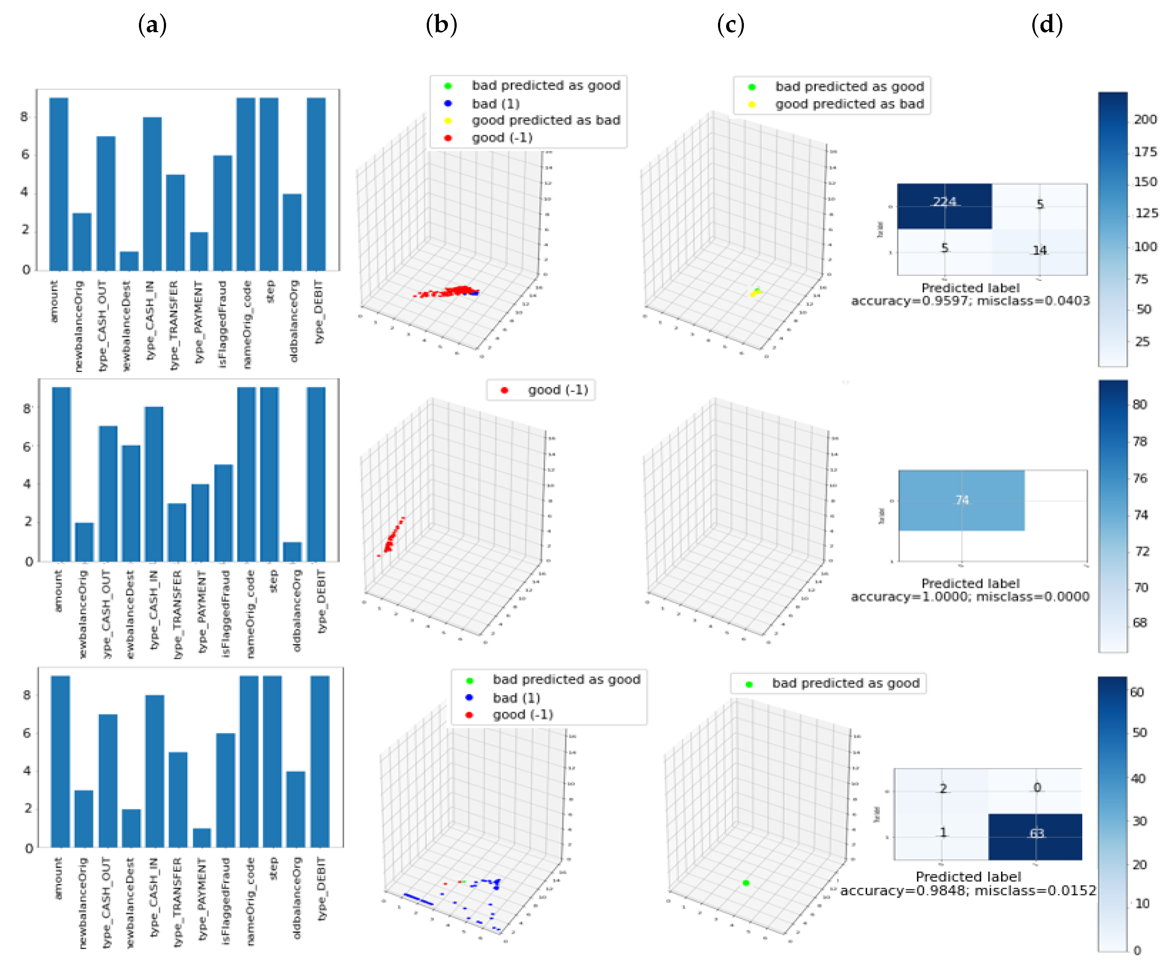
• We have verified the results obtained in the companion paper [1], that is, using the IVI algorithm with MIFF filter in a new real dataset, we can systematically capture all the real features with informative values.
• The better results obtained with the proposed approach (accuracy increase of 5%) suggested that the use of the presented method can improve the performance, meanwhile the reduction in terms of features simultaneously can enhance the computer efficiency.
• The use of STE has proven to be a suitable method to interpret the relationship between the contribution of each feature and the output of the classifier in black box methods.
• The use of ITR methods is proposed as a novel technique to classify transactions that are similar in terms of the participation of the variables in the classifier result.

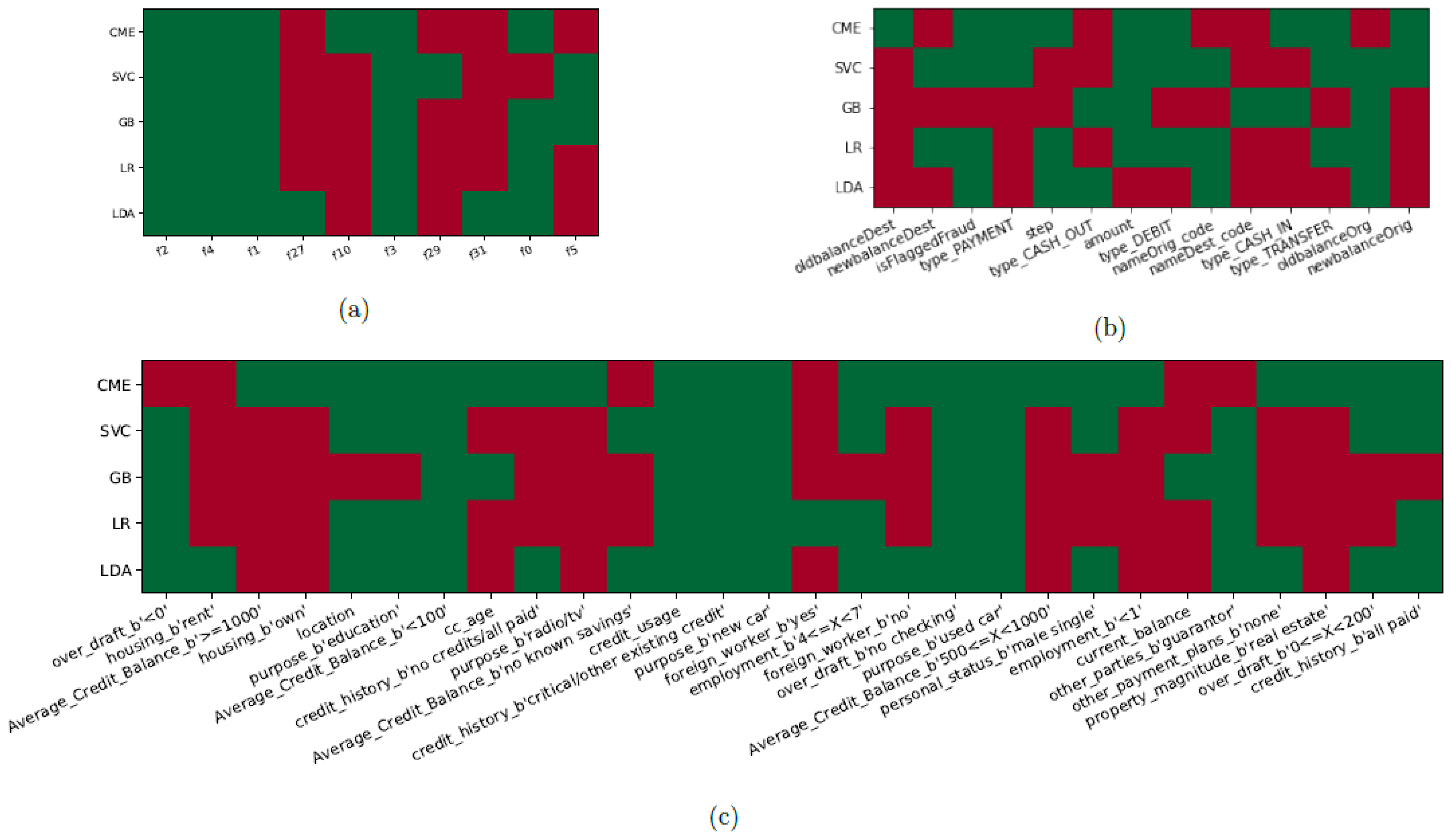
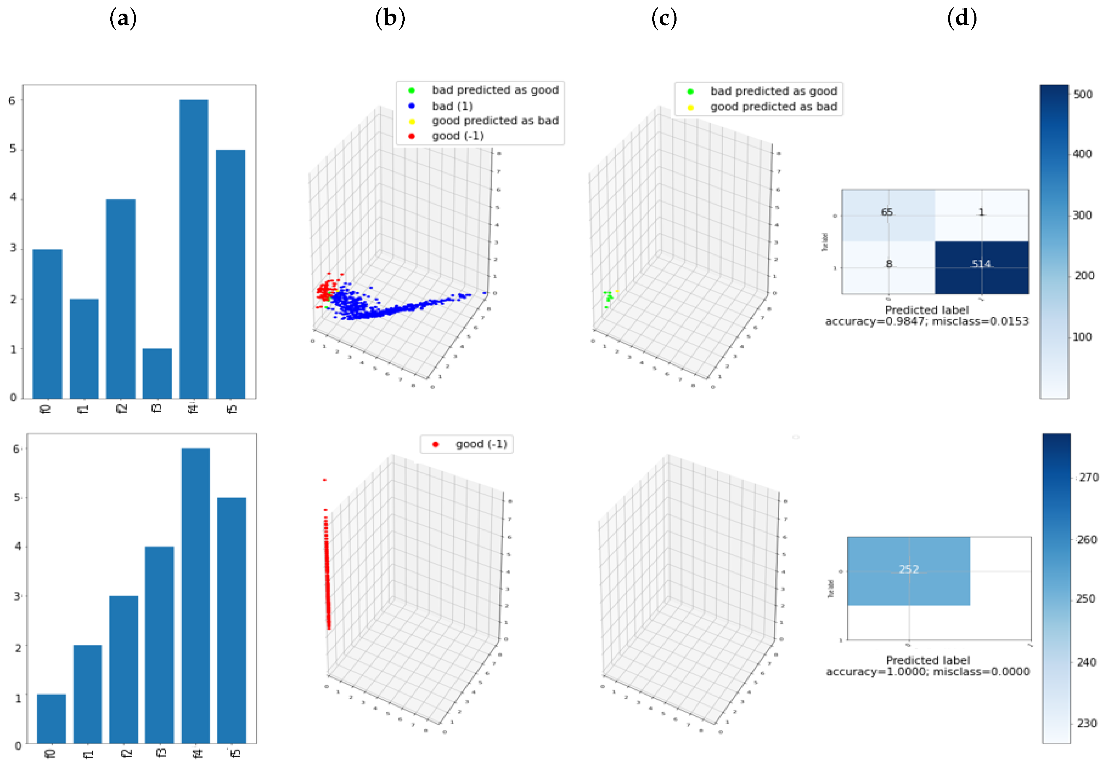
The results of applying these findings over the German Credit Dataset [47,48] were confirmed consistent with previous results in our synthetic dataset, as well as with other public published studies. It is also interesting to note that features picked by the model were consistent with those ones from published works sourcing the very same datasets [49,50]. Key features found in our case were livingbeyond means, lack or absence of transaction trail, unexpected overdrafts or declines in cash balances, and carloans. It is interesting to note that in the new dataset one of the features marked as relevant was isFlaggedFraud, which is a flag decided by a fraud analyst expert and it has high accuracy rate by itself.

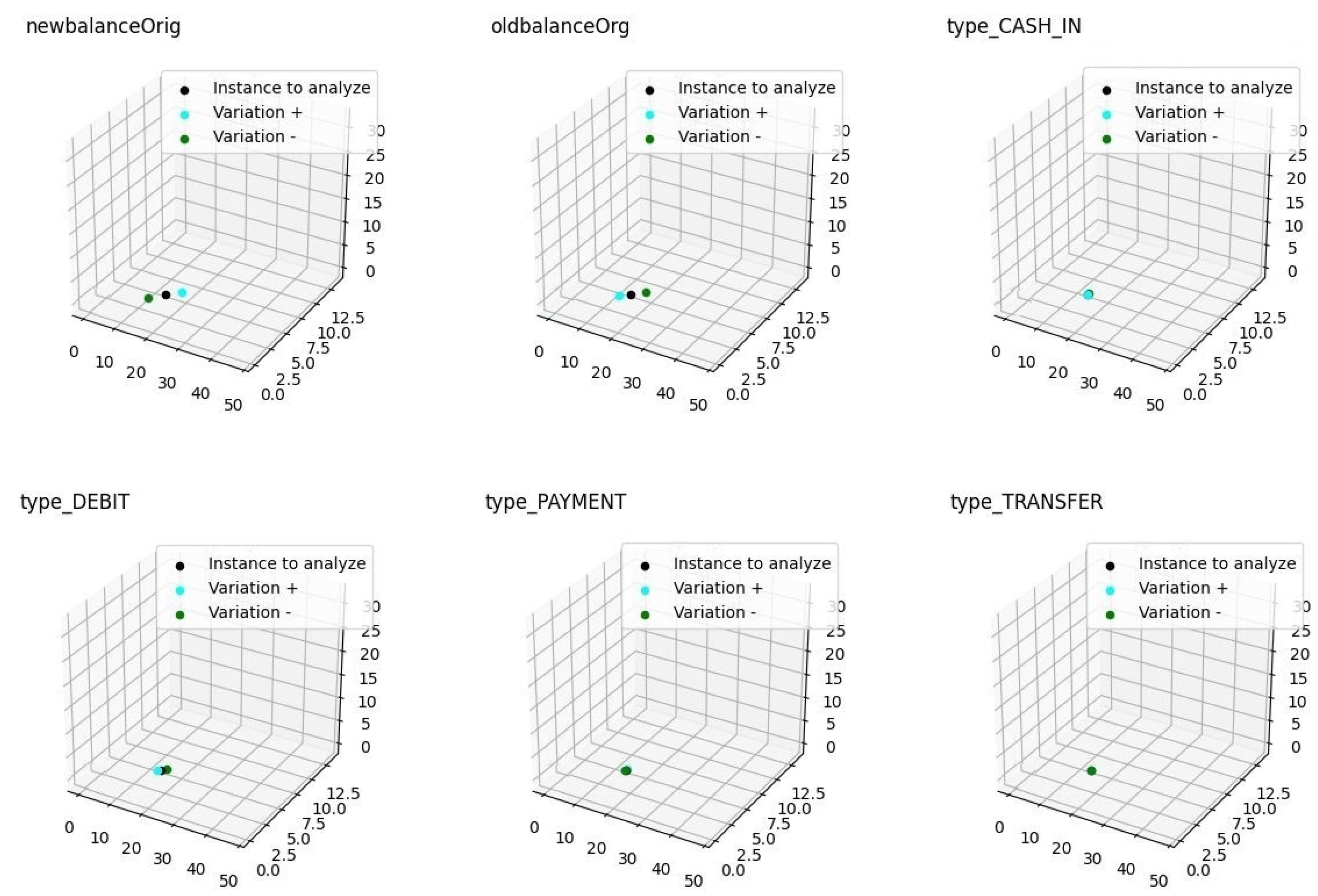
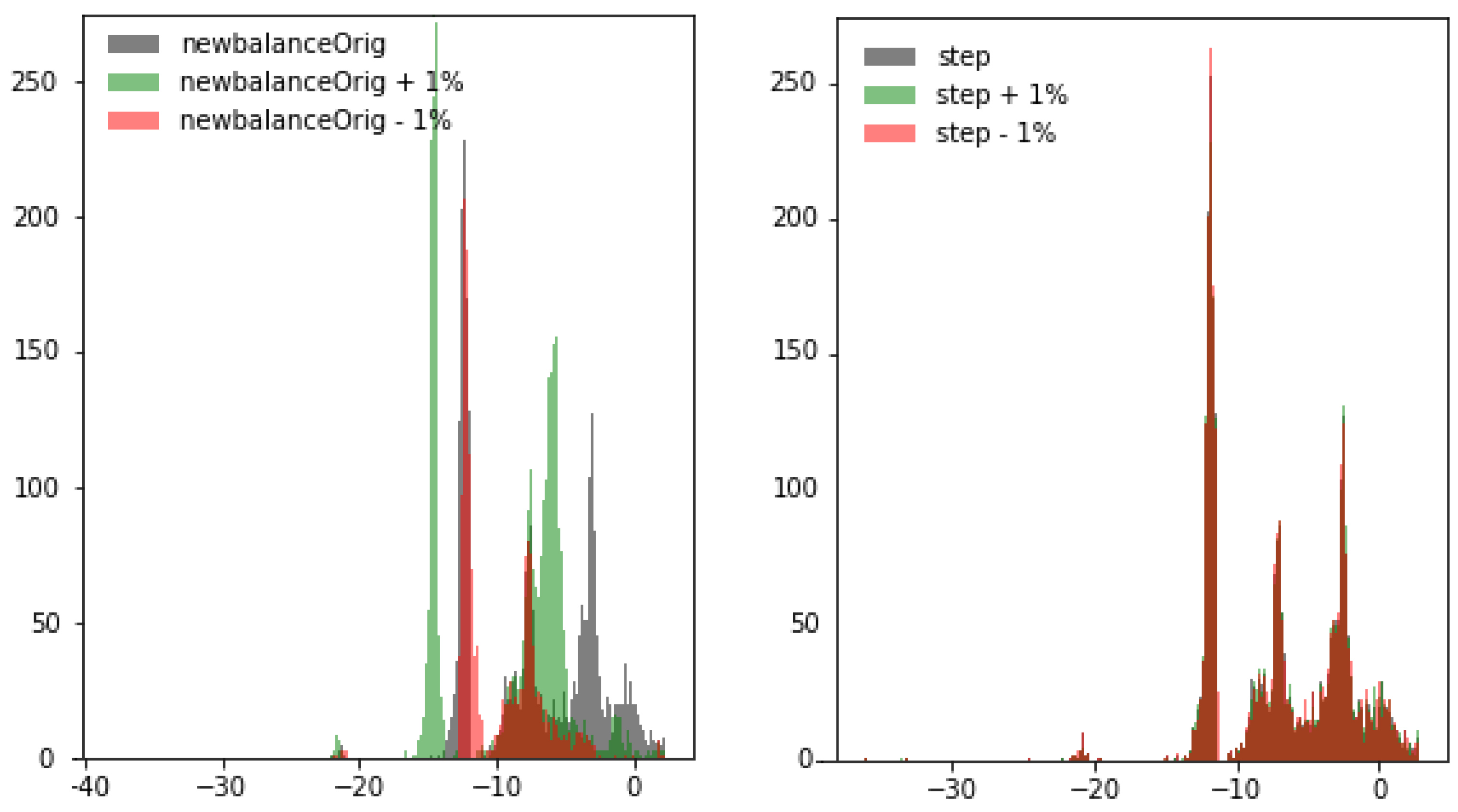
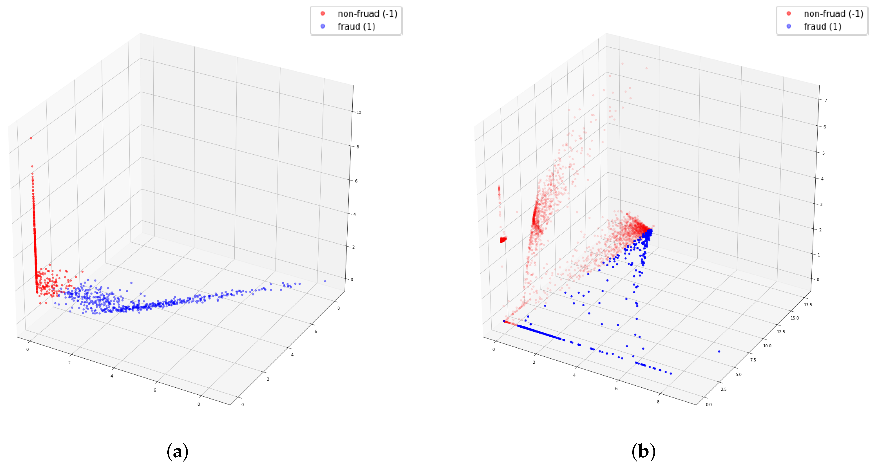
It was clear from the experiments that in the latent space the ML algorithms improve the classification task by better mapping the different types of transactions. The use of latent spaces could still be considered as a black-box model. With the aim of mitigating explanations for black-box, we have introduced two new mechanisms. First, STE summarizes the contribution of each feature for an individual transaction based on small-scale fluctuations, and second, the ITR method is able to build an individual feature ranking for each transaction. These rankings represent a closer estimation of those features that are more important than the others in the decision process for an individual transaction. The rationale of the ITR-based approach is a single-instance-level explanation for each transaction, which allows us to detect similar transaction profiles for the transaction with equivalent ITR. With these profiles, we can detect possible transaction biases caused by giving too much importance to not-allowed features, and then producing discrimination based on various categories including, for instance, race, sex, or marital status. We also may disclose the strong relation between STE and ITR. In the experiment where we verify how small variation in a feature in input space has different response in the latent space, we discovered that the feature newbalanceOrig has a high impact on this small variation, and this was confirmed when we generated the different profiles with ITR.

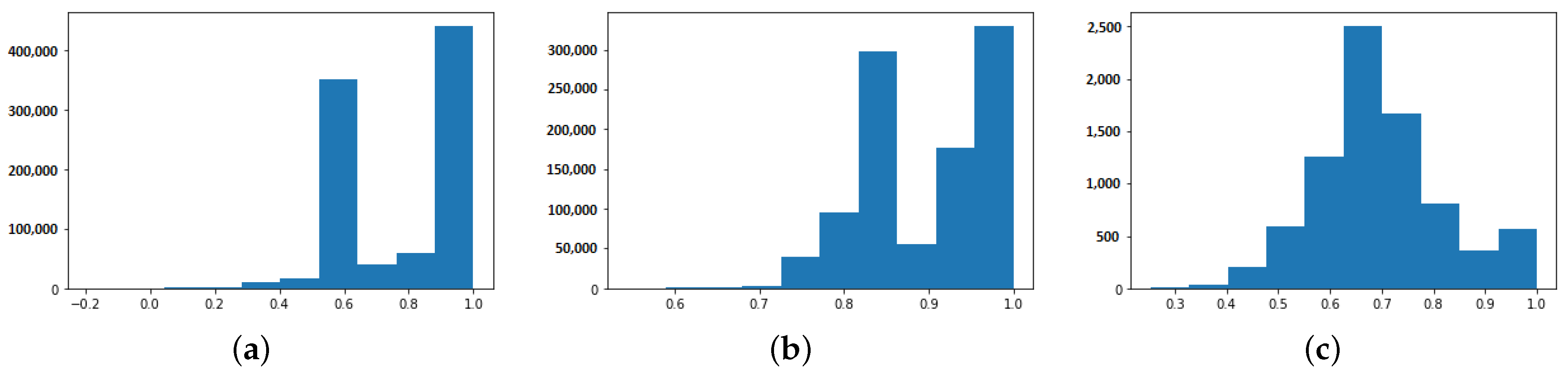
In addition to what is expressed in these conclusions regarding the potentiality in terms of the explicability shown, the evaluation of the Kendall correlation of ITR throughout the different datasets showed interesting results that encourage the deepening of the proposed analysis. In this sense, the differences in the means and distributions of the Kendall correlation, for the different datasets, can be interpreted in several directions. On the one hand is the existence of modalities in the distributions, which correspond to the existence of a number of different models needed to approximate the underlying reality that may be related to the number of different sets of transactions that take place. This set of transactions should not necessarily coincide with the classes under study, but with different realities, or varieties, which should be studied individually and separately for a better understanding of the sample base for greater interpretability. On the other hand, the presence of a single modality would indicate that of a linear, unique, and representative model, capable of evaluating with at least the same precision as the highly complex model evaluated. Thirdly, the existence of a non-modal distribution, whether uniform, Gaussian, or of any other type, could suggest various interpretations that in all cases could suggest facing new methods of analysis, either due to the existence of infinite linear models, equivalents, or a limited number of nonlinear models. In this direction, it is necessary to point out that although it is possible for each and every one of the transactions to obtain an ITR model, which provides interpretability to the proposed classification, it will be offered solely and exclusively for that transaction, not being possible to generalize to other cases. This local approximation and STE approach, could be understood as an advantage when it comes to interpretability, although its unique single explanation could also make regulators and authorities reluctant to validate extensively. That is why it is proposed, as the next step of this work, to advance in the knowledge of these distributions and the data models that give rise to them in order to also be able to propose interpretable and generalizable nonlinear models that ensure consistency, if not for the total of samples of the set, at least for a large group of them that are part of subsets that share the same ITR.

We can conclude that our methodology provides a detailed evaluation at the transaction level, adding interpretability to each transaction and making visible the most relevant features in decision process. This individualized, unbiased, and traceable perspective provides the necessary transparency, not only to comply with regulations, but also to be able to justify each classified transaction to clients and authorities.

As a general summary, we can affirm that the objective and contribution of this work was twofold. On the one hand, we intended to evaluate (and where appropriate, to improve) the detection capabilities of CFD techniques through the application of advanced AI techniques, which can be applied directly and in real time (online). Secondly, a novel analysis has been proposed, which is valid for any classification method providing interpretability retrospectively (offline). The authors consider that this last part constitutes the most important contribution of this work, since it is not only applicable to the latest generation CFD technique presented here, but, on the contrary, it can be used by regulators, clients, and authorities of supervision, as well as the entities themselves, separately and retrospectively (offline) to guarantee the non-discriminatory treatment and the audit of any pre-existing model without the need to delve into the details of CFD architecture.

The results and conclusions presented here also open up new potential lines of work for the future. In particular, (i) the possibility of extending the work carried out here to CFD risk assessments in real time (online); (ii) the possibility of deepening into ITR-clustering to better profile CFD; and, finally, (iii) to be able to extend AI techniques for fraud detection to their full potential, after having validated the blind evaluation techniques of black-box methods.

References

1. Chaquet-Ulldemolins, J.; Gimeno-Blanes, F.J.; Moral-Rubio, S.; Muñoz-Romero, S.; Rojo-Álvarez, J.L. On the Black-Box Challenge for Fraud Detection Using Machine Learning (I): Linear Models and Informative Feature Selection. Appl. Sci. 2022, 12, 3328. [Google Scholar] [CrossRef]
2. Buchanan, B.G. Artificial Intelligence In Finance; Technical Report; The Alan Turing Institute: London, UK, 2019. [Google Scholar]
3. Pascual, A. Future Proof Card Authorization; Technical Report; Javelin Strategy & Research: Pleasanton, CA, USA, 2015. [Google Scholar]
4. Dornadula, V.; Geetha, S. Credit Card Fraud Detection using Machine Learning Algorithms. Procedia Comput. Sci. 2019, 165, 631–641. [Google Scholar] [CrossRef]
5. Chandola, V.; Banerjee, A.; Kumar, V. Anomaly Detection: A Survey. ACM Comput. Surv. 2009, 41, 1–58. [Google Scholar] [CrossRef]
6. Ana, F. Artificial Intelligence In Financial Services; Technical Report; Banco de España: Madrid, Spain, 2019. [Google Scholar]
7. Yan, H.; Lin, S. New Trend in Fintech: Research on Artificial Intelligence Model Interpretability in Financial Fields. Open J. Appl. Sci. 2019, 9, 761–773. [Google Scholar] [CrossRef] [Green Version]
8. Wall, L. Some financial regulatory implications of artificial intelligence. J. Econ. Bus. 2018, 100, 55–63. [Google Scholar] [CrossRef]
9. Chen, C.; Lin, K.; Rudin, C.; Shaposhnik, Y.; Wang, S.; Wang, T. An Interpretable Model with Globally Consistent Explanations for Credit Risk. arXiv 2018, arXiv:1811.12615. [Google Scholar]
10. Wedge, R.; Kanter, J.M.; Veeramachaneni, K.; Rubio, S.M.; Perez, S.I. Solving the False Positives Problem in Fraud Prediction Using Automated Feature Engineering. In Machine Learning and Knowledge Discovery in Databases; Springer: Berlin/Heidelberg, Germany, 2019; pp. 372–388. [Google Scholar]
11. Machine Learning in UK Financial Services; Technical Report; Bank of England: London, UK, 2019.
12. Carvalho, D.; Pereira, E.; Cardoso, J. Machine Learning Interpretability: A Survey on Methods and Metrics. Electronics 2019, 8, 832. [Google Scholar] [CrossRef] [Green Version]
13. Muñoz-Romero, S.; Gorostiaga, A.; Soguero-Ruiz, C.; Mora-Jiménez, I.; Rojo-Álvarez, J.L. Informative variable identifier: Expanding interpretability in feature selection. Pattern Recognit. 2020, 98, 107077. [Google Scholar] [CrossRef]
14. Deshpande, P. Fraud Detection in Debit Card Transactions. Int. J. Sci. Res. Dev. 2015, 4, 263–270. [Google Scholar]
15. Pour, S.N.; Hosseini, S.; Hua, W.; Kangavari, M.R.; Zhou, X. SoulMate: Short-text author linking through Multi-aspect temporal-textual embedding. IEEE Trans. Knowl. Data Eng. 2019, 34, 448–461. [Google Scholar]
16. Hosseini, S.; Pour, S.N.; Cheung, N.; Kangavari, M.R.; Zhou, X.; Elovici, Y. TEALS: Time-Aware Text Embedding Approach to Leverage Subgraphs. 2019. Available online: http://xxx.lanl.gov/abs/1907.03191 (accessed on 24 August 2019).
17. Arora, S.; Li, Y.; Liang, Y.; Ma, T.; Risteski, A. Random Walks on Context Spaces: Towards an Explanation of the Mysteries of Semantic Word Embeddings. 2015. Available online: http://xxx.lanl.gov/abs/1502.03520 (accessed on 19 June 2019).
18. Dimitri, G.M.; Spasov, S.; Duggento, A.; Passamonti, L.; Lio’, P.; Toschi, N. Unsupervised stratification in neuroimaging through deep latent embeddings. In Proceedings of the 2020 42nd Annual International Conference of the IEEE Engineering in Medicine Biology Society (EMBC), Montreal, QC, Canada, 20–24 July 2020; pp. 1568–1571. [Google Scholar]
19. Tshitoyan, V.; Dagdelen, J.; Weston, L.; Dunn, A.; Rong, Z.; Kononova, O.; Persson, K.; Ceder, G.; Jain, A. Unsupervised word embeddings capture latent knowledge from materials science literature. Nature 2019, 571, 95–98. [Google Scholar] [CrossRef] [PubMed] [Green Version]
20. Gasparetti, F. Discovering prerequisite relations from educational documents through word embeddings. Future Gener. Comput. Syst. 2022, 127, 31–41. [Google Scholar] [CrossRef]
21. Pancino, N.; Graziani, C.; Lachi, V.; Sampoli, M.L.; Stefanescu, E.; Bianchini, M.; Dimitri, G.M. A Mixed Statistical and Machine Learning Approach for the Analysis of Multimodal Trail Making Test Data. Mathematics 2021, 9, 3159. [Google Scholar] [CrossRef]
22. Lin, S.Y.; Chiang, C.C.; Li, J.B.; Hung, Z.S.; Chao, K.M. Dynamic fine-tuning stacked auto-encoder neural network for weather forecast. Future Gener. Comput. Syst. 2018, 69, 446–454. [Google Scholar] [CrossRef]
23. Bengio, Y.; Lamblin, P.; Popovici, D.; Larochelle, H.; Montreal, U. Greedy layer-wise training of deep networks. Adv. Neural Inf. Process. Syst. 2007, 19, 153–160. [Google Scholar]
24. Bank, D.; Koenigstein, N.; Giryes, R. Autoencoders. 2020. Available online: http://xxx.lanl.gov/abs/2003.05991 (accessed on 3 April 2021).
25. Norlander, E.; Sopasakis, A. Latent Space Conditioning for Improved Classification and Anomaly Detection. 2019. Available online: http://xxx.lanl.gov/abs/1911.10599 (accessed on 28 November 2019).
26. Zamini, M.; Montazer, G. Credit Card Fraud Detection using autoencoder based clustering. In Proceedings of the 2018 9th International Symposium on Telecommunications (IST), Tehran, Iran, 17–19 December 2018; pp. 486–491. [Google Scholar]
27. Zou, J.; Zhang, J.; Jiang, P. Credit Card Fraud Detection Using Autoencoder Neural Network. 2019. Available online: http://xxx.lanl.gov/abs/1908.11553 (accessed on 30 August 2019).
28. Freitas, A. Comprehensible classification models: A position paper. Assoc. Comput. Mach. Sigkdd Explor. Newsl. 2014, 15, 1–10. [Google Scholar] [CrossRef]
29. Ribeiro, M.; Singh, S.; Guestrin, C. Why Should I Trust You? Explaining the Predictions of Any Classifier. 2016. Available online: http://xxx.lanl.gov/abs/1602.04938 (accessed on 9 August 2016).
30. Bertsimas, D.; Delarue, A.; Jaillet, P.; Martin, S. The Price of Interpretability. 2019. Available online: http://xxx.lanl.gov/abs/1907.03419 (accessed on 8 July 2019).
31. Yu, L.; Liu, H. Efficient Feature Selection via Analysis of Relevance and Redundancy. J. Mach. Learn. Res. 2004, 5, 1205–1224. [Google Scholar]
32. Venkatesh, B.; Anuradha, J. A review of feature selection and its methods. Cybern. Inf. Technol. 2019, 19, 3–26. [Google Scholar] [CrossRef] [Green Version]
33. Bellman, R. Adaptive Control Processes: A Guided Tour. (A RAND Corporation Research Study); Princeton University Press: Princeton, NJ, USA, 1961; pp. 255–260. [Google Scholar]
34. Chen, L. Curse of Dimensionality; Springer: Berlin/Heidelberg, Germany, 2009; pp. 545–546. [Google Scholar]
35. Torkkola, K. Feature Extraction by Non Parametric Mutual Information Maximization. J. Mach. Learn. Res. 2003, 3, 1415–1438. [Google Scholar]
36. Kohavi, R.; John, G.H. Wrappers for feature subset selection. Artif. Intell. 1997, 97, 273–324. [Google Scholar] [CrossRef] [Green Version]
37. Chen, X.; Jeong, J.C. Enhanced recursive feature elimination. In Proceedings of the Sixth International Conference on Machine Learning and Applications, University, OH, USA, 13–15 December 2007; pp. 429–435. [Google Scholar]
38. Tang, J.; Alelyani, S.; Liu, H. Feature selection for classification: A review. Data Classif. Algorithms Appl. 2014, 37, 37–64. [Google Scholar]
39. Dua, D.; Graff, C. UCI Machine Learning Repository. Data Retrieved from UCI. 2017. Available online: https://archive.ics.uci.edu/ml/datasets/statlog+(german+credit+data) (accessed on 17 November 1994).
40. Lopez-Rojas, E.A.; Elmir, A.; Axelsson, S. Paysim: A Financial Mobile Money Simulator for Fraud Detection. In Proceedings of the 28th European Modeling and Simulation Symposium, Larnaca, Cyprus, 26–28 September 2016. [Google Scholar]
41. Brause, R.; Langsdorf, T.; Hepp, M. Neural data mining for credit card fraud detection. In Proceedings of the 11th International Conference on Tools with Artificial Intelligence, Chicago, IL, USA, 9–11 November 1999; pp. 103–106. [Google Scholar]
42. Schölkopf, B.; Platt, J.; Hofmann, T. Advances in Neural Information Processing Systems 19: Proceedings of the 2006 Conference (Bradford Books); The MIT Press: Cambridge, MA, USA, 2007; pp. 153–160. [Google Scholar]
43. Baldi, P. Autoencoders, Unsupervised Learning, and Deep Architectures. In Proceedings of the ICML Workshop on Unsupervised and Transfer Learning, Bellevue, WA, USA, 27 July 2011; Guyon, I., Dror, G., Lemaire, V., Taylor, G., Silver, D., Eds.; PMLR: Norfolk, MA, USA, 2012; Volume 27, pp. 37–49. [Google Scholar]
44. Bengio, Y.; Guyon, G.; Dror, V.; Lemaire, G.; Taylor, D.; Silver, D. Deep Learning of Representations for Unsupervised and Transfer Learning. In Proceedings of the ICML Workshop on Unsupervised and Transfer Learning, Bellevue, WA, USA, 27 July 2011; Volume 7. [Google Scholar]
45. Käding, C.; Rodner, E.; Freytag, A.; Denzler, J. Fine-Tuning Deep Neural Networks in Continuous Learning Scenarios. In Proceedings of the Asian Conference on Computer Vision, Taipei, Taiwan, 20–24 November 2016; Springer: Cham, Switzerland, 2017; pp. 588–605. [Google Scholar]
46. Agrawal, P.; Girshick, R.; Malik, J. Analyzing the Performance of Multilayer Neural Networks for Object Recognition. In European Conference on Computer Vision; Springer: Cham, Switzerland, 2014; Volume 8695, pp. 329–344. [Google Scholar]
47. Pumsirirat, A.; Yan, L. Credit Card Fraud Detection using Deep Learning based on Auto-Encoder and Restricted Boltzmann Machine. Int. J. Adv. Comput. Sci. Appl. 2018, 9, 18–25. [Google Scholar] [CrossRef]
48. Gonzalez, J.; Holder, L.; Cook, D. Graph Based Concept Learning. In Proceedings of the FLAIRS Conference, Orlando, FL, USA, 22–24 May 2000. [Google Scholar]
49. Macailao, M. Raising the Red Flags: The Concept and Indicators of Occupational Fraud. J. Crit. Rev. 2020, 7, 26–29. [Google Scholar]
50. DiNapoli, T.P. Red Flags for Fraud. State of New York Office of the State Comptroller. State New York. Off. State Comptrol. 2008, 1, 1–14. [Google Scholar]
Figure 1. Architecture of an undercomplete autoencoder with a single encoding layer and a single decoding layer.
Applsci 12 03856 g001
Figure 3. Fine-tuning process. (a) Represents the autoencoder architecture. (b) Represents the encoder with an additional softmax layer. In this stage, we freeze the encoder layers and fit, allowing the gradient to backpropagate only through the softmax layer. (c) We again train the encoder and softmax layer, unfreezing the encoder layers. (d) We remove the softmax layer and we train the encoder and decoder freezing the encoders layers.
Applsci 12 03856 g003
Figure 4. Results of IVI algorithm for each ML technique in the synthetic dataset (a), in the German Credit Dataset (b), and in the PaySim (c). In rows are the different ML techniques: covariance multiplication estimator (CME), support vector machine classification (SVC), gradient boosting (GB), linear regression (LR), and linear discriminant analysis (LDA). In columns are the different features as defined previously. Green color represents scenarios where feature was identified as relevant. Red color represents features not identified as relevant during the analysis. The threshold for determining relevance is defined by MIFF filter (at least in two methods).
Applsci 12 03856 g004
Figure 5. Representation for one non-fraud transaction of how small variations for each feature in real space affect in the latent space with MIFF filter in the PaySim Dataset.
Applsci 12 03856 g005
Figure 6. Score distributions obtained in the latent spaces when small variations are applied for PaySim Dataset.
Applsci 12 03856 g006
Figure 7. Latent space for the different datasets. (a) Synthetic dataset. (b) PaySim Dataset. Red samples correspond to non-fraudulent transactions. Blue samples correspond to fraudulent instances. Fraud and non-fraud are easily observed in separate areas, although both groups are not always clearly separable.
Applsci 12 03856 g007
Figure 8. ITR analysis. By rows, the analysis of 2 sets of samples sharing same ITR for the synthetic dataset. By column: (a) represents the ITR, (b) latent space representation of the samples identifying the class and the AE prediction, (c) latent space of misclassified samples, (d) the confusion matrix for all the transactions sharing the same ITR.
Applsci 12 03856 g008
Figure 9. Different groups of ITR in PaySim Dataset. Column (a) represents the ITR. In column (b) we can see all the transaction with the same ITR with the class predicted with our methodology. Column (c) is similar to (b) but it only shows the mismatch. Finally, (d) shows the confusion matrix for all the transactions with the same ITR.
Applsci 12 03856 g009
Figure 10. Distribution. Kendall rank correlation coefficient for each dataset: (a) Synthetic dataset; (b) PaySim Dataset; (c) German Dataset.
Applsci 12 03856 g010