Article

Generative Adversarial Networks for Zero-Shot Remote Sensing Scene Classification

1
Aerospace Information Research Institute, Chinese Academy of Sciences, Beijing 100190, China
2
Key Laboratory of Network Information System Technology (NIST), Aerospace Information Research Institute, Chinese Academy of Sciences, Beijing 100190, China
3
School of Electronic, Electrical and Communication Engineering, University of Chinese Academy of Sciences, Beijing 100190, China
*
Author to whom correspondence should be addressed.
Appl. Sci. 2022, 12(8), 3760; https://doi.org/10.3390/app12083760
Submission received: 2 March 2022 / Revised: 30 March 2022 / Accepted: 6 April 2022 / Published: 8 April 2022
(This article belongs to the Special Issue Intelligent Computing and Remote Sensing)

Abstract

:
Deep learning-based methods succeed in remote sensing scene classification (RSSC). However, current methods require training on a large dataset, and if a class does not appear in the training set, it does not work well. Zero-shot classification methods are designed to address the classification for unseen category images in which the generative adversarial network (GAN) is a popular method. Thus, our approach aims to achieve the zero-shot RSSC based on GAN. We employed the conditional Wasserstein generative adversarial network (WGAN) to generate image features. Since remote sensing images have inter-class similarity and intra-class diversity, we introduced classification loss, semantic regression module, and class-prototype loss to constrain the generator. The classification loss was used to preserve inter-class discrimination. We used the semantic regression module to ensure that the image features generated by the generator can represent the semantic features. We introduced class-prototype loss to ensure the intra-class diversity of the synthesized image features and avoid generating too homogeneous image features. We studied the effect of different semantic embeddings for zero-shot RSSC. We performed experiments on three datasets, and the experimental results show that our method performs better than the state-of-the-art methods in zero-shot RSSC in most cases.

1. Introduction

Over the past decades, the epoch of remote sensing big data arrived, and remote sensing technology has made excellent progress [1]. It has played an important role in environmental monitoring [2], urban construction planning [3], and land use classification [4]. Currently, the accuracy of remote sensing image classification is very high. Most of the current remote sensing scene classification approaches rely on supervised learning [4,5,6], which can obtain excellent results when trained on large-scale datasets [7]. Usually, it requires labeling a lot of image data for each remote sensing image class. When we classify an image, the classifier does not work well if the category corresponding to the image is not in the training set, which is referred to as a zero-shot problem [8]. With the explosive growth of remote sensing image classes, we will encounter many new classes, and it is unrealistic to collect sufficient image samples for each class. It makes sense to identify the unseen class images when the training set does not contain the corresponding class, for instance, a rare aircraft species.
In order to overcome these problems in remote sensing images, it is of great interest to study zero-shot learning methods for RSSC. Zero-shot classification methods for remote sensing images are designed to address the classification for unseen category images, and more and more researchers are focusing on this topic. This can alleviate manual labeling, reduce a lot of labor, and make the existing classification model more scalable.
Humans can recognize about 30,000 object categories of information [8], and humans can transfer their knowledge to identify new classes when only textual descriptions of the new classes are available. The key of zero-shot learning to identify unseen classes is that zero-shot learning uses semantic and visual information from all image classes. Semantic information builds a bridge of knowledge transfer between seen and unseen categories, breaking the boundary of category mutual exclusion between training and testing sets.
The concept of zero-shot learning can be traced back to 2008 when Larochelle first introduced zero-shot learning [8]. Lampert et al. [9] first extended this approach to the field of computer vision. We can summarize the ZSL methods into two types: The first is embedding-based methods that map image features and semantic embeddings into one space and perform metric learning for ZSL. Zhang et al. [10] solved the zero-shot learning task by using the semantic similarity embedding (SSE) method. SSE fuses multiple semantic information into the same semantic space and calculates the similarity of them. Frome et al. [11] used a novel visual-semantic embedding approach to use annotated image data and semantic information from the unannotated text to recognize visual objects. Li et al. [12] presented a dual visual-semantic mapping framework for zero-shot classification (DMaP), which studies the relationship between the semantic space manifold and the transferability of visual-semantic mapping. However, they cannot work well in the generalized zero-shot learning (GZSL) setting because they overfit to seen classes. The second is GAN-based methods which generate fake image features for unseen classes and train KNN [13] or softmax classifier to perform ZSL. Xian et al. [14] first used generative adversarial networks (GANs) [15] to convert semantic features to visual features, providing a new idea for zero-shot learning. Felix et al. [16] mainly added a cycle consistency loss term, allowing GAN to generate more realistic images. Li et al. [17] introduced soul samples for generative zero-shot learning and used the cascade classifier to classify the unseen class. Yu et al. [18] presented an episode-based training pattern to improve the model’s performance for zero-shot learning. Generative adversarial networks (GANs) [15] is a popular zero-shot classification method. GAN-based methods generally work better than embedding-based methods.
For the remote sensing field, Li et al. [19] first proposed a zero-shot remote sensing scene classification (RSSC) method called ZSL-LP. ZSL-LP constructs a semantic-directed graph, then uses a label-propagation algorithm for zero-shot classification. Quan et al. [20] introduced a novel zero-shot RSSC method, which relies on Sammon embedding and spectral clustering. They modified semantic feature space class prototypes by Sammon embedding, which ensures the consistency with the visual feature space class prototypes. Wang et al. [21] introduced a distance-constrained semantic autoencoder for zero-shot remote sensing scene classification. Sumbul et al. [22] conducted a zero-shot study for fine-grained remote sensing image recognition. They first learned a compatible function and then showed how to transfer knowledge for unseen classes. Although these approaches have achieved promising results, most are devoted to designing visual-semantic embedding models only with seen classes, in which it is difficult to guarantee an excellent extension to unseen classes. In addition, these models trained only with seen data tend to misclassify unseen test instances into the seen category, generating a special imbalanced classification problem. Generative adversarial networks can alleviate the above issues to some extent [14,17,23]. As far as we know, no one has tried to apply generative adversarial networks for zero-shot RSSC. The GAN-based method designed for ordinary images cannot apply to remote sensing images well because remote sensing image scenes are complex. Remote sensing images generated by the GAN model may have instability and mode collapse problems. In addition, remote sensing images have inter-class similarity and intra-class diversity. Overall, zero-shot RSSC deserves more exploration.
We propose a novel approach for zero-shot RSSC with the mentioned considerations. Since the remote sensing image dataset does not directly provide class attribute information, we used four natural language processing models pre-trained on Wikipedia to obtain word vectors as the semantic information we need. Word2vec [24], Glove [25], Fasttext [26], and Bert [27] are the four natural language processing models. Because of the complexity of remote sensing scenes, we employed the conditional Wasserstein generative adversarial network [28] for generating image features directly instead of images to avoid instability and mode collapse problems in training. We trained a generator that can generate an arbitrary number of class image features from class semantic information, converting the zero-shot classification problem into a traditional classification problem. Following the characteristics of remote sensing images, we used the classification loss, semantic regression module, and class-prototype loss to constrain the generator to ensure the generator can generate image features close to the real image with the class semantic information. Our model is referred to as CSPWGAN. The classification loss is used to preserve inter-class discrimination. We used a semantic regression module to ensure that the image features generated by the generator can represent the semantic features. We introduced class-prototype loss when training the generator to constrain itself to ensure intra-class diversity of the synthesized image features and avoid generating too homogeneous image features. The contributions of this study are as follows:
1.
We trained a generator that can generate class image features close to the real image through class semantic information. We propose well-designed modules to constrain the generator, including classification loss module, class-prototype loss module, and semantic regression module. To the best of our knowledge, we are the first to employ generative adversarial networks for zero-shot remote sensing scene classification (RSSC);
2.
We explored the effect of different semantic embeddings for zero-shot RSSC. Specifically, we investigated various natural language processing models, i.e., Word2vec, Fasttest, Glove, and Bert, to extract semantic embeddings for each class either from the class name or from the class sentence descriptions. Our conclusion may help future work in understanding and choosing semantic embeddings for zero-shot RSSC;
3.
We conduct experiments on three benchmark datasets, UCM21 [29], AID30 [30] and NWPU45 [7]. The experimental results show that our method performs better than most state-of-the-art methods in zero-shot RSSC.

2. Methods

In this section, we first define the remote sensing image zero-shot classification task. Then we present our generative framework for zero-shot RSSC. Finally, we introduce each part of the model in detail.

2.1. Problem Definition

Let D = x i , y i , e ( y i ) i = 1 N where D denotes the dataset, x is the features of remote sensing images, y is the class label of remote sensing images, e ( y ) denotes the classes semantic feature. The dataset D is split into the seen and unseen datasets. Let D s = x s i , y s i , e ( y s i ) i = 1 N s represent the seen datasets and D u = x u i , y u i , e ( y u i ) i = 1 N u represent the unseen datasets. Class label set y includes the seen class label set y s and unseen class label set y u . The seen class label set y s is disjointed y u . The relationship can be represented by y = y s y u and y s y u = ϕ . The purpose of the ZSL task is to predict the class label y u , and the purpose of the GZSL task is to predict the class label y.

2.2. Overall Framework

In this section, we present the overall framework of our CSPWGAN model. As shown in Figure 1, our model is composed of two parts, including the Class Semantic Feature Representation Module and the Feature Generation Module.
Class Semantic Feature Representation Module. Typical zero-shot task datasets usually contain class attribute vectors [9]. Since there are no class attribute vectors in the remote sensing image dataset, we used the natural language pre-training model to generate the word vectors we need.
Feature Generation Module. We used a generative model to train a generator that can generate class image features by class semantic features, which can convert the zero-shot remote sensing scene classification problem into a traditional classification problem and avoid the hubness problem [31]. In addition, using generative adversarial networks can prevent the class imbalance problem under the GZSL setting. Meanwhile, we considered that remote sensing images have inter-class similarity and intra-class diversity. We used the classification loss, semantic regression module, and class-prototype loss to constrain the generator. The classification loss was used to preserve inter-class discrimination. We used semantic regression module to ensure that the image features generated by the generator can represent the semantic features. To ensure intra-class diversity of the synthesized image features and avoid generating too homogeneous image features, we introduced class-prototype loss to constrain the generator. The key to solving this problem is to obtain a high-performance generator, and multiple losses to jointly constrain the generator to obtain better results.

2.3. Class Semantic Feature Representation Module

Zero-shot learning aims to solve the problem of recognizing unseen classes that cannot be accomplished by traditional supervised learning. The key is that zero-shot learning uses not only visual features but also class semantic features. Class semantic information builds a bridge of knowledge transfer between seen and unseen categories, breaking the boundary of category mutual exclusion between training and testing sets. There are usually two ways to extract semantic features: attribute vectors and word embeddings.
Attributes vectors are manually annotated using expert knowledge and share attribute space among all classes of objects. It is the most common and efficient method of semantic feature construction. Attribute vectors can leverage prior human knowledge with good interpretability and accuracy. At the same time, the disadvantage of attribute vectors is that they are highly dependent on manual annotation and are challenging to annotate in the absence of prior human knowledge.
Using natural language pre-training models to generate the word vectors we need has the advantage of being fast, simple, and does not require prior knowledge. Word2vec [24], Glove [25], Fasttext [26], and Bert [27] are the most common methods used. These methods can be trained with open-source corpora (e.g., Wikipedia), which significantly saves the cost of manual annotation. We can use them to convert classes name or class text descriptions into word vectors. For example, we can use Word2vec to convert remote sensing image classes name into 300- or 500-dimensional word vectors and use Bert to convert the description of remote sensing image classes into 768-dimensional word vectors.

2.4. Feature Generation Module

Since there are no samples of unseen categories in the training data, it is difficult to train a classifier for unseen categories. Our method synthesizes unseen classes’ image visual features through class semantic information and noise vectors. We trained a classifier that can classify unseen class images based on the synthesized image features and their corresponding unseen class labels. Our approach was inspired by [14]. CSPWGAN is composed of a generative adversarial network. The generative adversarial network model converts the zero-shot RSSC problem into a traditional classification problem.
We used the conditional generative adversarial net [32] as our baseline model. The network is composed of a generative model G and a discriminative model D that compete in a two-player minimax game. G generates the visual image representation x ^ by its semantic feature e ( y ) and a noise vector sampled from a normal distribution z N ( 0 , I ) . The generation process can be represented as: y × z x . We used the semantic feature e ( y ) and a noise vector z as inputs of G, and x ^ of the class label y as outputs of G. θ G denotes the parameters of G. The discriminative model D can be represented as: e × x [ 0 , 1 ] , θ D denotes the parameters of D. D aims to accurately distinguish the real image visual feature x from the generated visual features x ^ . θ D denotes the parameters of the discriminative model D. G aims to cheat the discriminator D by generating images that can be mistaken for the real ones. This is the training process for estimating the parameters of θ D and θ G .
Our model only uses the seen class data for training, but it can also generate image features of unseen classes. Generating models are usually hard to train and not easy to stabilize. We used a stable training methods called WGAN [28], the loss function of WGAN is as follows:
L W G A N = E [ D ( x , e ( y ) | θ D ) ] E [ D ( x ^ , e ( y ) | θ D ) ] λ E [ ( x ^ D ( x ˜ , e ( y ) ) 2 1 ) 2 ]
where E [ . ] denotes the expectation function. x ^ = G ( z , e ( y ) | θ G ) , x ˜ = β x + ( 1 β ) x ^ with β U ( 0 , 1 ) . Both G and D are multilayer networks. λ represents the penalty factor. We set λ = 10 in this study.
To achieve good optimization, we applied classification loss, semantic regression module and class-prototype loss to train the network.
Classification Loss. Because of the complexity of remote sensing images, the WGAN model cannot ensure that the generated samples are discriminative enough. Generating inaccurate samples results in the bad performance of the classifier. To alleviate this issue, we added a classifier to identify whether the generated image features can be classified into the correct class. By doing this, the generated features are more discriminative. We added a simple classifier that uses the negative log-likelihood:
L C = E x ^ p x ^ [ l o g P ( y | x ^ ; θ ) ]
where x ^ = G ( z , e ( y ) | θ G ) , the class label of x ^ is y, and P ( y | x ^ ; θ ) represents the probability that the class label of x ^ predicted by the classifier is its true label y. θ is pre-trained on the seen classes dataset. It can be represented as:
P ( y | x ^ ; θ ) = exp ( ( θ ) T x ^ ) c y exp ( ( θ ) T x ^ )
Semantic Regression Module. We used class semantic features to guide the generator to generate image features for the corresponding class. The generator is trained using seen class semantic features and visual features in the training phase, and using unseen class semantic features synthesizes unseen visual features in the testing phase. Finally, we converted the zero-shot classification problem into a traditional classification problem. Our model relies on a high-performance generator that aims to generate image features similar to real image features. We used the semantic features of the unseen class to synthesize image features; if it differs significantly from the real image feature distribution, the synthesized image features cannot represent the real image features of the class. The classifier trained with synthetic image features of unseen categories misclassifies the real unseen class images. We must ensure that the image features generated by the generator are similar to the real image features, which allows us to achieve higher recognition results for the unseen categories. We were inspired by [16], and used the semantic regression module to constrain the generator. This can be represented as:
L S R = E x P r [ e ( y ) R ( G ( z , e ( y ) | θ G ) | θ R ) 2 2 ]
where R denotes the regressor, and θ R denotes the parameters of R. θ R is pre-trained on seen classes using the following function:
L R = min θ R e ( y ) R ( x | θ R ) 2 2
Class-Prototype Loss. In remote sensing images, the features of different sample images in the same class vary greatly and have diversity within the class. We used classification loss, the semantic regression module cannot guarantee that the image features synthesized by the generator are diverse. To ensure that the synthesized image features are more consistent with the distribution of real remote sensing image features and avoid the generated image features being too homogeneous, we introduced class-prototype loss in training to constrain the generator. We were inspired by [17]. First, we clustered each class of real remote sensing image features to obtain k clusters. We obtained class prototype sample image features by averaging all sample image features in each group, and can obtain k class prototype samples for each real remote sensing image class. In the training process, we hoped that the image features synthesized by the generator would be close to at least one class prototype vector in the same class.
Let X n y denote the nth cluster of category y, each category has k clusters. In this study, we set k = 5 for simplicity. Let p n y denote the nth prototype vector of category y, each category has k prototype vectors. The p n y is defined as:
p n y = 1 N n y x i X n y x i
where N n y denotes the number of samples in cluster X n y . For the generated fake features x ^ , we also define the prototype vector p ^ n y as:
p ^ n y = 1 N n y x ^ i X ^ n y x ^ i
We hope that each sample x ^ generated for the category y is be close to at least one prototype vector p y . This loss can be defined as:
L 1 = 1 n i = 1 n min j [ 1 , k ] x ^ i p j y 2 2
where n represents the number of generated samples for the category y and k represents the number of prototype vectors per class. We also hope that the prototype vector of generated fake features p ^ n y is close to at least a real prototype vector p n y for the same class, which is formulated as:
L 2 = 1 n y y = 1 n y min j [ 1 , k ] p ^ j y p j y 2 2
where n y represents the number of all categories. Our class-prototype loss can be expressed by the following equation:
L C P L = λ 1 L 1 + λ 2 L 2
With this class-prototype loss for constraint, our model can avoid generating single-view image features and ensure the intra-class diversity of the synthesized image features for remote sensing images.
Finally, our model was trained with the following overall loss function:
min θ G max θ D L W G A N + α L C + β L S R + λ L C P L
where α , β , and λ are hyperparameters of the model to balance the importance of each term.

2.5. Training and Testing

In the training phase, the generator was trained using class semantic features and visual features from the seen categories. We used classification loss, semantic regression module, and class-prototype loss to constrain the generator. We used classification loss to allow the generator to learn to generate discriminative image features. We used the semantic regression module to ensure that the generated image features represent semantic features. Class-prototype loss ensures that the synthetic image features are more consistent with the distribution of real remote sensing image features. The model is trained with Equation (11).
After the training is complete, we repeated the generator to generate an arbitrary number of image features for each unseen category. We obtained a training set of synthetic images. In the ZSL task, we can classify the unseen images by the classifier trained on this dataset. In the GZSL task, we added the synthetic images dataset to the seen class dataset and trained a classifier to recognize both seen and unseen class images. We can choose a softmax classifier or KNN, etc. In this study, we used the softmax classifier.

3. Results

In this section, we designed experiments to evaluate our method. First, we introduced the remote sensing image datasets used in our experiments. Second, we introduced our experimental setup. Third, we exploited the effect of our method on different semantic vectors. Fourth, we compared our approach with the current state-of-the-art zero-shot RSSC method. Finally, we performed ablation studies.

3.1. Dataset

We selected three datasets in the most widely used remote sensing images classification datasets, namely UCM21 [29], AID30 [30] and NWPU45 [7].
The UCM21 dataset has 21 classes, and each scene class consists of 100 images. For each scene class, the size of the image is 256 × 256 pixels. The AID30 dataset has 30 categories, each category has 200 to 400 samples, and each sample has a pixel size of 600 × 600 . The NWPU45 dataset has 45 classes, and each scene class consists of 700 images. For each scene class, the size of the image is 256 × 256 pixels. As shown in Figure 2, we can see the diversity of images within the same class.

3.2. Evaluation Protocols

In the ZSL task, we used the class average accuracy [14] as the performance evaluation metric, i.e., the classification accuracy within a class is first counted for each class. Then the class average accuracy is calculated by finding the mean value.
In the GZSL task, harmonic mean accuracy [14] is used to evaluate the classification effect. The formula for calculating the harmonic mean accuracy is as follows:
H = 2 × u × s u + s
where u denotes the accuracy of unseen classes, s denotes the accuracy of seen classes, and H denotes the harmonic mean accuracy.

3.3. Implementation Details

We first must extract image features, obtain the corresponding class semantic information, and then use the GAN network for training. We used the ResNet-101 model pre-trained on ImageNet to extract 2048-dimensional features of remote sensing images. We obtained the word vectors of the corresponding class by using Word2vec, Glove, Fasttext, and Bert. We implemented our model via multilayer neural networks. The generator G contains a 4096 nodes hidden layer activated by LeakyRelu [33], the output layer has 2048 nodes activated by Relu [34]. The discriminator D also contains a 4096 nodes hidden layer activated by LeakyRelu, and the output layer has no activation. The regressor R contains a 2048 nodes hidden layer, the dimensionality of the output layer is the same as the semantic information dimension. We used the adam [35] optimizer to optimize our model, l r = 0.0001 , β 1 = 0.5, and β 2 = 0.999. In this study, we set α = 0.001 , β = 10 , γ = 1 , γ 1 = 0.01 , γ 2 = 0.001 . The above algorithms were implemented using the PyTorch, and the experiments were completed on four RTX2080s.

3.4. Ablations on Different Word Vectors

We used four natural language processing models pre-trained on Wikipedia to obtain word vectors for remote sensing datasets. Moreover, we obtained different dimensional word vectors for each method as class semantic features. To find the word vectors with the best results, we compared the word vectors obtained by these four methods with different dimensions. The classification results on the UCM21 dataset are shown in Figure 3.
The Word2vec model pre-trained on Wikipedia has three dimensions, i.e., 100, 300, and 500, and they correspond to an accuracy of 0.6097, 0.5698, and 0.6266, respectively.
The Glove model pre-trained on Wikipedia has four dimensions, i.e., 50, 100, 200, and 300, and they correspond to an accuracy of 0.5455, 0.5602, 0.5294, and 0.5236, respectively.
The Fasttext model pre-trained on Wikipedia has four dimensions, i.e., 50, 100, 200, 300, and they correspond to an accuracy of 0.5264, 0.5358, 0.5325, and 0.5166, respectively.
We used Bert in two ways to obtain word vectors, one using class names and the other using class description texts, which correspond to an accuracy of 0.4536 and 0.3978, respectively.
We also explored the effect of different word vectors in GZSL tasks. We used Word2vec-500, Glove-100, Fastetext-100, and Bert-768 as semantic information In Table 1. When we used the Word2vec method to extract 500-dimensional word vectors as semantic information for remote sensing image datasets, we achieved the best results in both ZSL and GZSL tasks.

3.5. Comparison with State-of-the-Art

To show the superiority of CSPWGAN, we present a comparison of our method with some previous methods. We chose these baselines: SSE [10], DMaP [12], SAE [36], ZSL-LP [19], ZSC-SA [20], DASE [21], VSC [37], VSOP [38], f-CLSWGAN [14], CYCLEWGAN [16], and RBGN [39].
SSE [10] fuses multiple semantic information into the same semantic space and calculates the similarity of them. DMaP [12] studies the relationship between the semantic space manifold and the transferability of visual-semantic mapping. SAE [36] is based on learning a Semantic autoencoder for solving the label prediction problem. SAE adds a constraint from visual mapping to semantic features to alleviate the domain drift problem. ZSL-LP [19] constructs a semantic-directed graph, then uses a label-propagation algorithm for zero-shot classification. ZSC-SA [20] is a novel zero-shot RSSC method, which relies on Sammon embedding and spectral clustering. VSC [37] employs a novel visual architecture constraint for ZSL. VSOP [38] proposes to match latent visual and semantic representations in a shared subspace. DASE [21] proposes a distance-constrained semantic autoencoder to handle ZSRSSC. RBGN [39] employs an adversarial attack and bidirectional generation into GZSL to improve the generalizability and robustness of the model.
For a fair comparison with prior methods, we divided the dataset into four seen/unseen ratios, and each ratio was randomly divided 25 times, and 25 zero-shot classification experiments were performed. The average accuracy of the categories is taken as the result. Regarding the splitting ratio setting of the remote sensing dataset, our method is consistent with previous zero-shot classification methods for remote sensing images, such as articles DSAE, ZSC-SA, and ZSL-LP. Table 2, Table 3 and Table 4 show the classification results for UCM21, AID30, and NWPU45 datasets. As shown in Table 2, Table 3 and Table 4, our method significantly improved the classification accuracy compared with the state-of-the-art(sota) approaches for zero-shot RSSC in most cases. On the UCM21 dataset, our method improved 4.03%, 8.69%, 9.58%, and 5.99% under different seen/unseen ratios (e.g., 16/5, 13/8, 10/11, and 7/14, respectively). On the AID30 dataset, our method improves 2.37%, 2.61%, 1.05%, and 1.78% under different seen/unseen ratios (e.g., 25/5, 20/10, 15/15, and 10/20, respectively). On the NWPU45 dataset, our method improves 0.24% and 1.45% under two seen/unseen ratios (e.g., 25/20 and 20/25, respectively). The standard deviation of our method is smaller than DSAE in most cases, which also proves the superiority of our method. In conclusion, the results show that our method is more adapted for remote sensing images. The results also show that our method works better with a higher ratio of unseen classes and higher accuracy.
To compare the classification performance for each unseen category, we fixed the unseen classes for a given split ratio according to the DSAE setting. We present the confusion matrix of our approach and the DASE method. Notably, each column of the matrix represents an instance of the real class, and each row of the matrix represents an instance of the predicted class. On the UCM21 dataset, we have five unseen classes with the seen/unseen ratio set to 16/5, i.e., “freeway”, “golf course”, “intersection”, “medium residential”, and “storage tanks”. Figure 4 shows the confusion matrix of the DASE method and our method on the UCM21 datasets. We found that we obtained 27% and 22% improvement on the classes “freeway” and “storage tanks”, respectively. Our method has a decrease in classification accuracy on other unseen classes, but the average accuracy of the five unseen classes is higher than DASE. The average accuracy of our method improved from 63.6% to 68.8% on the five unseen categories. On the AID30 dataset, we have five unseen classes with the seen/unseen ratio set to 25/5, i.e., “dense residential”, “desert”, “forest”, “industrial”, and “pond”. Figure 5 shows the confusion matrix of the DASE method and our method on the AID30 datasets. We achieved 31% and 80% improvement on the classes “dense residential” and “forest”, respectively. The average accuracy of our method improved from 64.8% to 72.4% on the five unseen categories. On the NWPU45 dataset, we have ten unseen classes with the seen/unseen ratio set to 35/10, i.e., “airport”, “basketball court”, “circular farmland”, “cloud”, “dense residential”, “desert”,“harbor”, “intersection”, “medium residential” and “sparse residential”. Figure 6 shows the confusion matrix of the DASE method and our method on the NWPU45 datasets. We achieved 2%, 5%, 60%, 16%, and 1% improvement on the classes “airport”, “circular farmland”, “dense residential”, “medium residential” and “sparse residential”, respectively.
To visually display the efficiency of CSPWGAN, we visualized the synthesized image features through our CSPWGAN method and the original image features of the unseen class in Figure 7. We used the popular t-SNE [40] tool to display the synthesized image features and the real image features. From Figure 7, we can observe that the unseen image features synthesized by our method are relatively close to the real image feature distribution, which proves that our approach is meaningful.

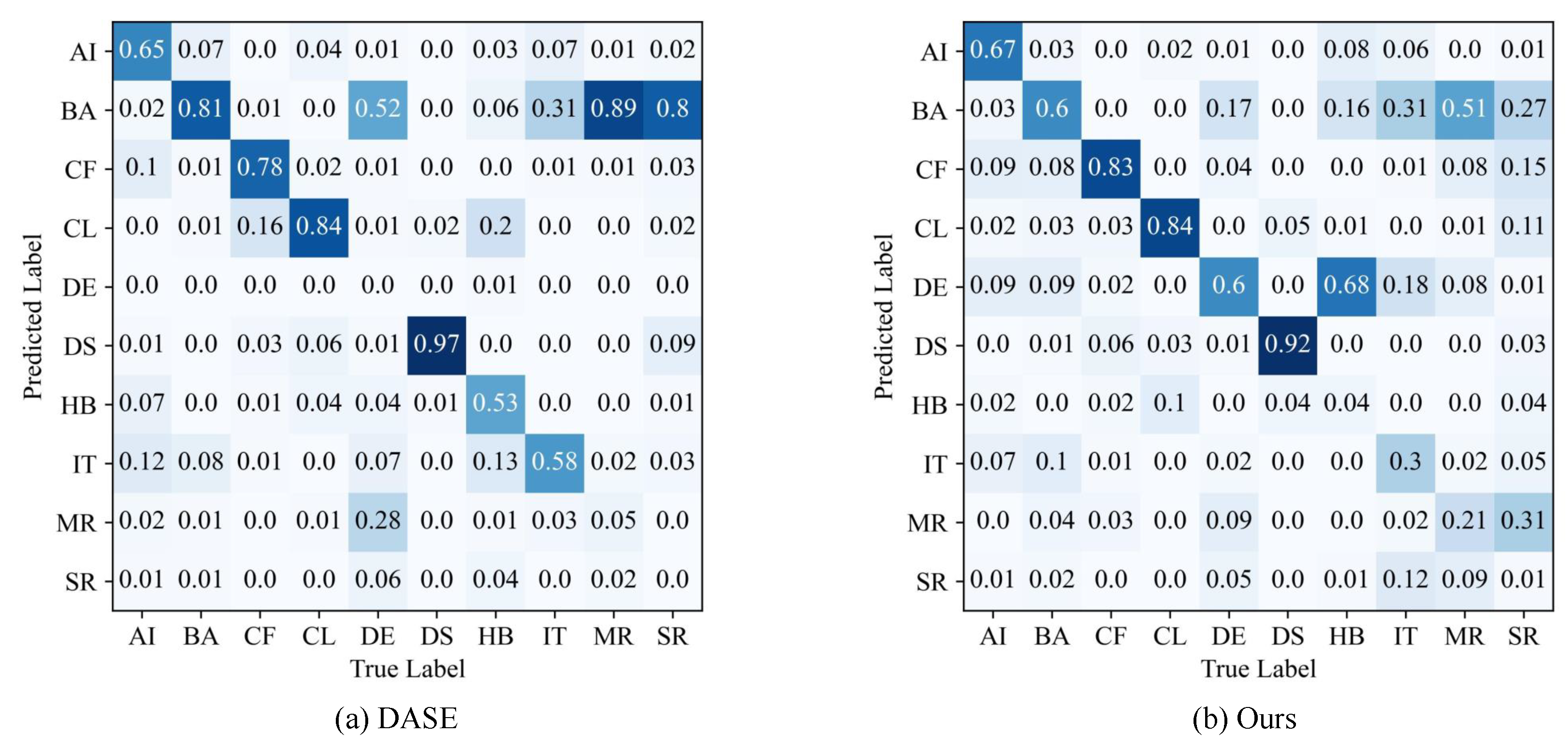
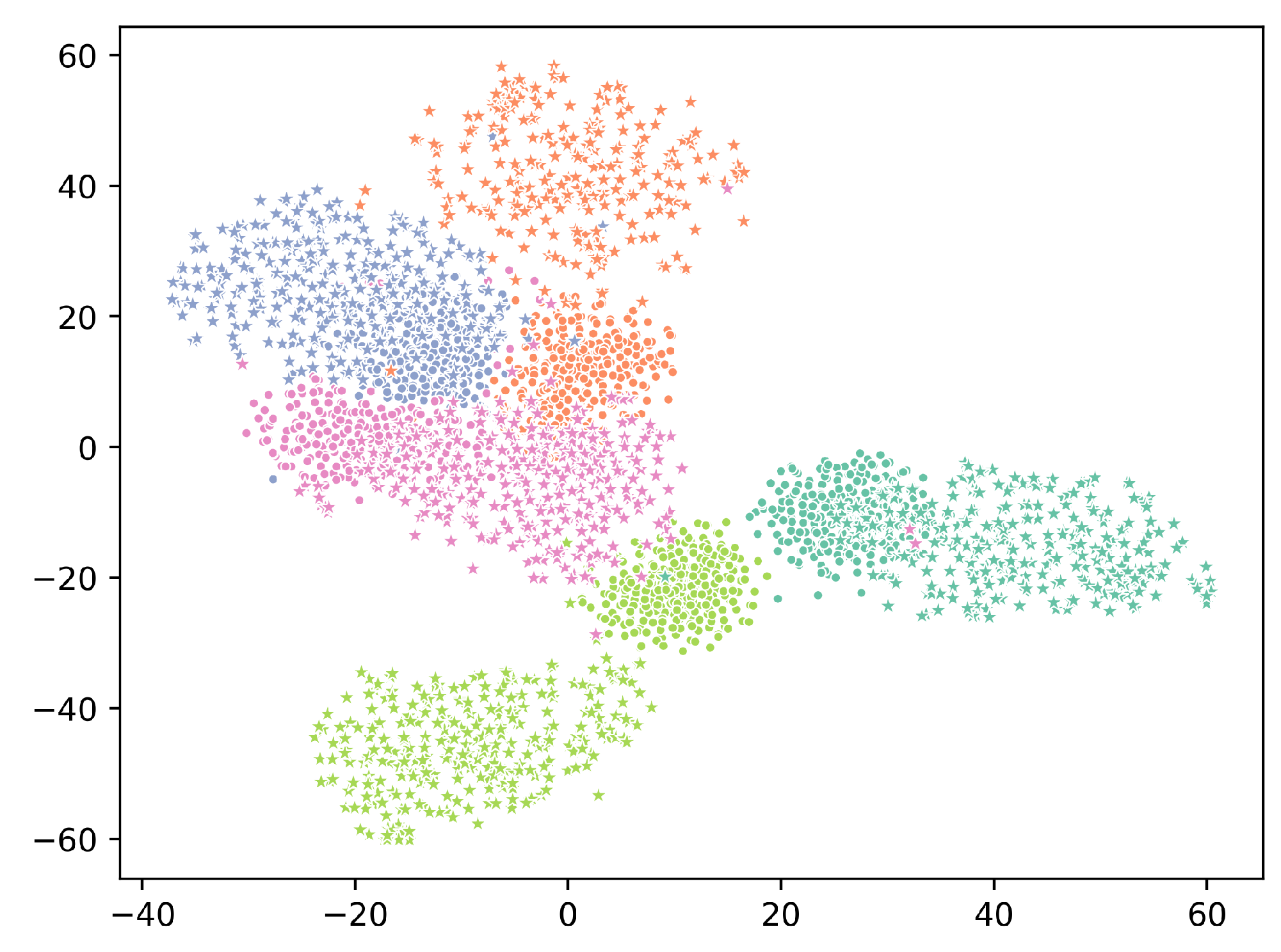
3.6. Ablation Studies

Our approach is based on generative adversarial networks. Following the characteristics of remote sensing images, we used classification loss, class-prototype loss, and semantic regression loss to constrain the generator, to ensure that we can obtain a high-performance generator. We constructed ablation experiments to understand our model further and to evaluate their effects. We set λ = 0 in (12), our model without classification loss term can be referred to as CSPWGAN- λ ; we set β = 0 in (12), our model without semantic regression term can be referred to as CSPWGAN- β ; we set γ = 0 in (12), our model without class-prototype loss term can be referred to as CSPWGAN- γ . We executed ablation experiments on the UCM21, AID30, and NWPU45 datasets. Table 5 shows the result of ablation studies on the UCM21, AID30, and NWPU45 datasets. On the UCM21 dataset, when we removed the classification loss item, the model accuracy decreased by 2.82%; when we removed the semantic regression term, the model accuracy decreased by 2.23%; when we removed the semantic regression term, the model accuracy decreased by 2.99%. The results show the effectiveness of the three items for zero-shot RSSC. We can find the same conclusion on the AID30 and NWPU45 datasets.

4. Conclusions

This study presents a novel method for zero-shot remote sensing scene classification (RSSC) named CSPWGAN. We are the first to apply generative adversarial networks for zero-shot RSSC. Since the remote sensing image dataset does not directly provide class attribute information, we used four natural language processing models pre-trained on Wikipedia to obtain word vectors as the class semantic information we need. We used generative adversarial networks to train a generator that can generate class image features through class semantic features, converting the zero-shot RSSC problem into a traditional classification problem. Following the characteristics of remote sensing images, we used the classification loss, semantic regression module, and class-prototype loss to constrain the generator. The classification loss was used to preserve inter-class discrimination. We used a semantic regression module to ensure the image features generated by the generator can represent the semantic features. We introduced class-prototype loss when training the generator to constrain itself to ensure intra-class diversity of the synthesized image features and avoid generating too homogeneous image features. We conducted experiments on two benchmark datasets. The results demonstrate the superiority of our proposed CSPWGAN method for remote sensing images. Our method can work better with a high ratio of unseen classes. In the experiments, we found that the class semantic information significantly affects the classification results. In future work, we will try to obtain better class semantic vectors and use a better approach to reduce classification standard deviation and improve the classification accuracy for remote sensing images.
In future work, we can also try to use active learning [41] to solve the problem of unseen remote sensing image classes in the training data. The key idea of active learning (AL) is that if a machine-learning algorithm is allowed to select the data it learns, then it can achieve higher accuracy with fewer labeled training instances. Active learning retrieves the most useful unlabeled data from a large set of unlabeled data, hands it over to a professional for labeling, and then uses that sample to train the model to improve its accuracy. Many excellent methods have emerged in the field of remote sensing and deep learning using active learning, such as [42,43,44]. Our approach uses semantic and visual information from all image classes. Class semantic information builds a bridge of knowledge transfer between seen and unseen categories, breaking the boundary of category mutual exclusion between training and testing sets. Active learning and our model are two different ideas for solving the problem of addressing unseen classes in the training data.

Author Contributions

Conceptualization, Z.L., D.Z., Y.W. and D.L.; methodology, Z.L. and D.Z.; software, Z.L., Y.W. and J.Z.; validation, Z.L., D.L. and J.Z.; formal analysis, Z.L.; investigation, Z.L.; resources, Z.L. and J.Z.; data curation, Z.L. and D.Z.; writing—original draft preparation, Z.L., Y.W. and D.L.; writing—review and editing, Z.L. and D.Z.; visualization, Z.L.; supervision, D.Z.; project administration, D.Z. All authors have read and agreed to the published version of the manuscript.

Funding

This research received no external funding.

Institutional Review Board Statement

Not applicable.

Informed Consent Statement

Not applicable.

Data Availability Statement

Conflicts of Interest

The authors declare no conflict of interest.

References

  1. Chi, M.; Plaza, A.; Benediktsson, J.A.; Sun, Z.; Shen, J.; Zhu, Y. Big data for remote sensing: Challenges and opportunities. Proc. IEEE 2016, 104, 2207–2219. [Google Scholar] [CrossRef]
  2. Cheng, G.; Guo, L.; Zhao, T.; Han, J.; Li, H.; Fang, J. Automatic landslide detection from remote-sensing imagery using a scene classification method based on BoVW and pLSA. Int. J. Remote Sens. 2013, 34, 45–59. [Google Scholar] [CrossRef]
  3. Qi, K.; Yang, C.; Hu, C.; Shen, Y.; Shen, S.; Wu, H. Rotation invariance regularization for remote sensing image scene classification with convolutional neural networks. Remote Sens. 2021, 13, 569. [Google Scholar] [CrossRef]
  4. Castelluccio, M.; Poggi, G.; Sansone, C.; Verdoliva, L. Land use classification in remote sensing images by convolutional neural networks. arXiv 2015, arXiv:1508.00092. [Google Scholar]
  5. Hu, F.; Xia, G.S.; Hu, J.; Zhang, L. Transferring deep convolutional neural networks for the scene classification of high-resolution remote sensing imagery. Remote Sens. 2015, 7, 14680–14707. [Google Scholar] [CrossRef] [Green Version]
  6. Penatti, O.A.; Nogueira, K.; Dos Santos, J.A. Do deep features generalize from everyday objects to remote sensing and aerial scenes domains? In Proceedings of the IEEE Conference on Computer Vision and Pattern Recognition Workshops, Boston, MA, USA, 7–12 June 2015; pp. 44–51. [Google Scholar]
  7. Cheng, G.; Han, J.; Lu, X. Remote sensing image scene classification: Benchmark and state of the art. Proc. IEEE 2017, 105, 1865–1883. [Google Scholar] [CrossRef] [Green Version]
  8. Larochelle, H.; Erhan, D.; Bengio, Y. Zero-Data Learning of New Tasks; AAAI: Menlo Park, CA, USA, 2008; Volume 1, p. 3. [Google Scholar]
  9. Lampert, C.H.; Nickisch, H.; Harmeling, S. Attribute-based classification for zero-shot visual object categorization. IEEE Trans. Pattern Anal. Mach. Intell. 2013, 36, 453–465. [Google Scholar] [CrossRef]
  10. Zhang, Z.; Saligrama, V. Zero-shot learning via semantic similarity embedding. In Proceedings of the IEEE international conference on computer vision, Santiago, Chile, 7–13 December 2015; pp. 4166–4174. [Google Scholar]
  11. Frome, A.; Corrado, G.S.; Shlens, J.; Bengio, S.; Dean, J.; Ranzato, M.; Mikolov, T. Devise: A deep visual-semantic embedding model. In Proceedings of the Advances in Neural Information Processing Systems 26 (NIPS 2013), Stateline, NV, USA, 5–10 December 2013; Volume 26. [Google Scholar]
  12. Li, Y.; Wang, D.; Hu, H.; Lin, Y.; Zhuang, Y. Zero-shot recognition using dual visual-semantic mapping paths. In Proceedings of the IEEE Conference on Computer Vision and Pattern Recognition, Honolulu, HI, USA, 21–26 July 2017; pp. 3279–3287. [Google Scholar]
  13. Fix, E.; Hodges, J.L. Discriminatory analysis. Nonparametric discrimination: Consistency properties. Int. Stat. Rev. Int. Stat. 1989, 57, 238–247. [Google Scholar] [CrossRef]
  14. Xian, Y.; Lorenz, T.; Schiele, B.; Akata, Z. Feature generating networks for zero-shot learning. In Proceedings of the IEEE Conference on Computer Vision and Pattern Recognition, Salt Lake City, UT, USA, 18–23 June 2018; pp. 5542–5551. [Google Scholar]
  15. Goodfellow, I.; Pouget-Abadie, J.; Mirza, M.; Xu, B.; Warde-Farley, D.; Ozair, S.; Courville, A.; Bengio, Y. Generative adversarial nets. In Proceedings of the Advances in Neural Information Processing Systems 27 (NIPS 2014), Montréal, QC, Canada, 8–13 December 2014; Volume 27. [Google Scholar]
  16. Felix, R.; Reid, I.; Carneiro, G. Multi-modal cycle-consistent generalized zero-shot learning. In Proceedings of the European Conference on Computer Vision (ECCV), Munich, Germany, 8–14 September 2018; pp. 21–37. [Google Scholar]
  17. Li, J.; Jing, M.; Lu, K.; Ding, Z.; Zhu, L.; Huang, Z. Leveraging the invariant side of generative zero-shot learning. In Proceedings of the IEEE/CVF Conference on Computer Vision and Pattern Recognition, Long Beach, CA, USA, 15–20 June 2019; pp. 7402–7411. [Google Scholar]
  18. Yu, Y.; Ji, Z.; Han, J.; Zhang, Z. Episode-based prototype generating network for zero-shot learning. In Proceedings of the IEEE/CVF Conference on Computer Vision and Pattern Recognition, Seattle, WA, USA, 13–19 June 2020; pp. 14035–14044. [Google Scholar]
  19. Li, A.; Lu, Z.; Wang, L.; Xiang, T.; Wen, J.R. Zero-shot scene classification for high spatial resolution remote sensing images. IEEE Trans. Geosci. Remote Sens. 2017, 55, 4157–4167. [Google Scholar] [CrossRef]
  20. Quan, J.; Wu, C.; Wang, H.; Wang, Z. Structural alignment based zero-shot classification for remote sensing scenes. In Proceedings of the 2018 IEEE International Conference on Electronics and Communication Engineering (ICECE), Xi’an, China, 10–12 December 2018; pp. 17–21. [Google Scholar]
  21. Wang, C.; Peng, G.; De Baets, B. A Distance-Constrained Semantic Autoencoder for Zero-Shot Remote Sensing Scene Classification. IEEE J. Sel. Top. Appl. Earth Obs. Remote Sens. 2021, 14, 12545–12556. [Google Scholar] [CrossRef]
  22. Sumbul, G.; Cinbis, R.G.; Aksoy, S. Fine-grained object recognition and zero-shot learning in remote sensing imagery. IEEE Trans. Geosci. Remote Sens. 2017, 56, 770–779. [Google Scholar] [CrossRef] [Green Version]
  23. Verma, V.K.; Arora, G.; Mishra, A.; Rai, P. Generalized zero-shot learning via synthesized examples. In Proceedings of the IEEE Conference on Computer Vision and Pattern Recognition, Salt Lake City, UT, USA, 18–23 June 2018; pp. 4281–4289. [Google Scholar]
  24. Mikolov, T.; Chen, K.; Corrado, G.; Dean, J. Efficient estimation of word representations in vector space. arXiv 2013, arXiv:1301.3781. [Google Scholar]
  25. Pennington, J.; Socher, R.; Manning, C.D. Glove: Global vectors for word representation. In Proceedings of the 2014 Conference on Empirical Methods in Natural Language Processing (EMNLP), Doha, Qatar, 25–29 October 2014; pp. 1532–1543. [Google Scholar]
  26. Joulin, A.; Grave, E.; Bojanowski, P.; Mikolov, T. Bag of tricks for efficient text classification. arXiv 2016, arXiv:1607.01759. [Google Scholar]
  27. Devlin, J.; Chang, M.W.; Lee, K.; Toutanova, K. Bert: Pre-training of deep bidirectional transformers for language understanding. arXiv 2018, arXiv:1810.04805. [Google Scholar]
  28. Arjovsky, M.; Chintala, S.; Bottou, L. Wasserstein generative adversarial networks. In Proceedings of the International Conference on Machine Learning, Sydney, Australia, 6–11 August 2017; pp. 214–223. [Google Scholar]
  29. Yang, Y.; Newsam, S. Bag-of-visual-words and spatial extensions for land-use classification. In Proceedings of the 18th SIGSPATIAL International Conference on Advances in Geographic Information Systems, San Jose, CA, USA, 2–5 November 2010; pp. 270–279. [Google Scholar]
  30. Xia, G.S.; Hu, J.; Hu, F.; Shi, B.; Bai, X.; Zhong, Y.; Zhang, L.; Lu, X. AID: A benchmark data set for performance evaluation of aerial scene classification. IEEE Trans. Geosci. Remote Sens. 2017, 55, 3965–3981. [Google Scholar] [CrossRef] [Green Version]
  31. Shigeto, Y.; Suzuki, I.; Hara, K.; Shimbo, M.; Matsumoto, Y. Ridge regression, hubness, and zero-shot learning. In Proceedings of the Joint European Conference on Machine Learning and Knowledge Discovery in Databases, Porto, Portugal, 7–11 September 2015; Springer: Berlin/Heidelberg, Germany, 2015; pp. 135–151. [Google Scholar]
  32. Mirza, M.; Osindero, S. Conditional generative adversarial nets. arXiv 2014, arXiv:1411.1784. [Google Scholar]
  33. Maas, A.L.; Hannun, A.Y.; Ng, A.Y. Rectifier nonlinearities improve neural network acoustic models. In Proceedings of the 30th International Conference on Machine Learning, ICML 2013, Atlanta, GA, USA, 16–21 June 2013; Volume 30, p. 3. [Google Scholar]
  34. Nair, V.; Hinton, G.E. Rectified linear units improve restricted boltzmann machines. In Proceedings of the 27th International Conference on Machine Learning, Haifa, Israel, 21–24 June 2010. [Google Scholar]
  35. Kingma, D.P.; Ba, J. Adam: A method for stochastic optimization. arXiv 2014, arXiv:1412.6980. [Google Scholar]
  36. Kodirov, E.; Xiang, T.; Gong, S. Semantic autoencoder for zero-shot learning. In Proceedings of the IEEE Conference on Computer Vision and Pattern Recognition, Honolulu, HI, USA, 21–26 July 2017; pp. 3174–3183. [Google Scholar]
  37. Wan, Z.; Chen, D.; Li, Y.; Yan, X.; Zhang, J.; Yu, Y.; Liao, J. Transductive zero-shot learning with visual structure constraint. In Proceedings of the Advances in Neural Information Processing Systems 32 (NeurIPS 2019), Vancouver, BC, Canada, 8–14 December 2019; Volume 32. [Google Scholar]
  38. Wu, H.; Yan, Y.; Chen, S.; Huang, X.; Wu, Q.; Ng, M.K. Joint visual and semantic optimization for zero-shot learning. Knowl.-Based Syst. 2021, 215, 106773. [Google Scholar] [CrossRef]
  39. Xing, Y.; Huang, S.; Huangfu, L.; Chen, F.; Ge, Y. Robust bidirectional generative network for generalized zero-shot learning. In Proceedings of the 2020 IEEE International Conference on Multimedia and Expo (ICME), London, UK, 6–10 July 2020; pp. 1–6. [Google Scholar]
  40. Van der Maaten, L.; Hinton, G. Visualizing data using t-SNE. J. Mach. Learn. Res. 2008, 9, 2579–2605. [Google Scholar]
  41. Settles, B. Active Learning Literature Survey; University of Wisconsin-Madison: Madison, WI, USA, 2009. [Google Scholar]
  42. Fu, M.; Yuan, T.; Wan, F.; Xu, S.; Ye, Q. Agreement-Discrepancy-Selection: Active Learning with Progressive Distribution Alignment. In Proceedings of the AAAI Conference on Artificial Intelligence, Palo Alto, CA, USA, 2–9 February 2021; Volume 35, pp. 7466–7473. [Google Scholar]
  43. Wang, S.; Li, Y.; Ma, K.; Ma, R.; Guan, H.; Zheng, Y. Dual adversarial network for deep active learning. In Proceedings of the European Conference on Computer Vision, Glasgow, UK, 23–28 August 2020; Springer: Berlin/Heidelberg, Germany, 2020; pp. 680–696. [Google Scholar]
  44. Ahmad, M.; Khan, A.; Khan, A.M.; Mazzara, M.; Distefano, S.; Sohaib, A.; Nibouche, O. Spatial prior fuzziness pool-based interactive classification of hyperspectral images. Remote Sens. 2019, 11, 1136. [Google Scholar] [CrossRef] [Green Version]
Figure 1. The framework of our proposed CSPWGAN model for zero-shot RSSC.
Applsci 12 03760 g001
Figure 2. Some remote sensing sample images in UCM21, AID30, and NWPU45 datasets.
Applsci 12 03760 g002
Figure 3. The classification accuracy of different word vectors on the UCM21 dataset.
Applsci 12 03760 g003
Figure 4. Confusion matrix of the two methods on the UCM21 dataset. Where “FW”, “GC”, “IT”, “MR”, and “ST” denotes “freeway”, “golf course”, “intersection”, “medium residential”, and “storage tanks”, respectively.
Applsci 12 03760 g004
Figure 5. Confusion matrix of the two methods on the AID30 dataset. Where “DR”, “DE”, “FO”, “IN”, and “PO” denotes “dense residential”, “desert”, “forest”, “industrial”, and “pond”, respectively.
Applsci 12 03760 g005
Figure 6. Confusion matrix of the two methods on the NWPU45 dataset. Where “AI”, “BA”, “CF”, “CL”, “DE”, “DS”, “HB”, “IT”, “MR”, and “SR” denotes “airport”, “basketball court”, “circular farmland”, “cloud”, “dense residential”, “desert”,“harbor”, “intersection”, “medium residential” and “sparse residential”, respectively.
Applsci 12 03760 g006
Figure 7. t-SNE visualizations of image features for five unseen classes on the AID30 dataset. The pentagram denotes the real features of the unseen class. The solid circle denotes the synthetic features of the unseen class. The real and synthetic features of the same unseen class have the same color.
Applsci 12 03760 g007
Table 1. The experimental results of different word vectors. Bold font denotes the best result.
Word2vecGloveFasttextBertUC Merced Land Use Dataset
accusH
0.62660.48690.73480.5857
0.56020.43030.73890.5439
0.53580.40070.68750.5063
0.45360.35070.71380.4704
Table 2. With different seen/unseen ratios, the average ZSL classification accuracies and standard deviation (%) of our CSPWGAN model and the sota methods on the UCM21 dataset. Bold font denotes the best result.
Method16/513/810/117/14
SSE [10]35.59 ± 5.9023.42 ± 3.8117.07 ± 3.5610.82 ± 2.10
DMaP [12]48.92 ± 8.7130.91 ± 4.7722.99 ± 4.8117.30 ± 3.04
SAE [36]49.50 ± 8.4232.71 ± 6.4924.04 ± 4.3618.63 ± 2.76
ZSL-LP [19]49.01 ± 8.8531.26 ± 5.0923.28 ± 4.1317.55 ± 2.90
ZSC-SA [20]50.42 ± 8.8434.12 ± 6.1024.68 ± 4.2218.38 ± 2.74
VSC [37]55.91 ± 11.7736.26 ± 7.3125.97 ± 5.7919.53 ± 3.05
VSOP [38]46.48 ± 7.8329.81 ± 4.5621.97 ± 4.1116.14 ± 2.59
f-CLSWGAN [14]56.97 ± 11.0636.47 ± 6.2827.89 ± 4.9919.34 ± 3.96
CYCLEWGAN [16]58.36 ± 10.0436.81 ± 5.5328.37 ± 4.5321.15 ± 3.51
RBGN [39]57.93 ± 11.5636.95 ± 5.9927.74 ± 5.1620.67 ± 3.95
DSAE [21]58.63 ± 11.2337.50 ± 7.7925.59 ± 5.2420.18 ± 3.07
CSPWGAN (our)62.66 ± 10.7946.19 ± 5.5235.17 ± 4.9326.17 ± 3.87
Table 3. With different seen/unseen ratios, the average ZSL classification accuracies and standard deviation (%) of our CSPWGAN model and the sota methods on the AID30 dataset. Bold font denotes the best result.
Method25/520/1015/1510/20
SSE [10]46.11 ± 7.2130.28 ± 4.9019.94 ± 2.4312.73 ± 1.27
DMaP [12]43.40 ± 7.2928.29 ± 4.7819.38 ± 2.6211.56 ± 1.29
SAE [36]47.34 ± 8.4232.12 ± 4.4523.73 ± 3.2813.77 ± 1.17
ZSL-LP [19]46.77 ± 7.6530.82 ± 4.9021.78 ± 3.3712.97 ± 1.06
ZSC-SA [20]50.87 ± 8.7433.46 ± 5.9924.41 ± 3.8315.89 ± 2.03
VSC [37]52.61 ± 8.3735.85 ± 5.5226.11 ± 3.7617.50 ± 2.19
VSOP [38]48.56 ± 7.9032.95 ± 5.5224.84 ± 3.0414.03 ± 2.47
f-CLSWGAN [14]50.68 ± 11.2533.89 ± 5.7224.95 ± 2.9617.26 ± 3.06
CYCLEWGAN [16]52.37 ± 10.4735.94 ± 5.4625.28 ± 2.6617.89 ± 2.86
RBGN [39]51.99 ± 11.3236.27 ± 5.6524.83 ± 3.0716.83 ± 3.14
DSAE [21]53.49 ± 8.5835.32 ± 5.1725.92 ± 3.9217.65 ± 2.52
CSPWGAN (our)55.86 ± 10.6037.93 ± 5.2626.97 ± 2.5319.43 ± 3.02
Table 4. With different seen/unseen ratios, the average ZSL classification accuracies and standard deviation (%) of our CSPWGAN model and the sota methods on the NWPU45 dataset. Bold font denotes the best result.
Method35/1030/1525/2020/25
SSE [10]33.36 ± 3.5823.30 ± 2.4816.88 ± 2.2912.94 ± 1.46
DMaP [12]49.53 ± 6.3138.07 ± 4.8328.15 ± 3.8623.95 ± 2.60
SAE [36]44.81 ± 4.7335.07 ± 3.9124.65 ± 3.7120.77 ± 2.02
ZSL-LP [19]47.00 ± 6.6436.45 ± 4.5826.71 ± 3.4322.90 ± 2.47
ZSC-SA [20]48.40 ± 6.3637.55 ± 4.5428.27 ± 3.4723.69 ± 2.38
VSC [37]50.68 ± 6.6040.92 ± 4.5930.62 ± 3.1025.51 ± 2.04
VSOP [38]45.32 ± 5.7136.09 ± 4.6325.44 ± 3.1322.18 ± 2.00
f-CLSWGAN [14]45.35 ± 6.3738.97 ± 4.9330.06 ± 2.9624.31 ± 2.57
CYCLEWGAN [16]46.87 ± 5.9939.85 ± 4.7131.17 ± 2.6625.06 ± 2.74
RBGN [39]44.68 ± 6.1440.31 ± 4.8931.91 ± 3.0724.89 ± 2.44
DSAE [21]51.52 ± 6.9141.94 ± 4.6131.85 ± 3.3225.20 ± 2.17
CSPWGAN (our)50.66 ± 5.8641.61 ± 4.4832.09 ± 2.9626.65 ± 2.33
Table 5. Ablation results on the UCM21, AID30, and NWPU45 datasets.
MethodUCM21AID30NWPU45
CSPWGAN- λ 59.84 ± 9.6453.05 ± 10.0747.82 ± 6.24
CSPWGAN- β 60.43 ± 10.3253.79 ± 10.3448.79 ± 5.67
CSPWGAN- γ 59.67 ± 9.8552.89 ± 9.5947.07 ± 5.96
CSPWGAN62.66 ± 10.7955.86 ± 10.6050.66 ± 5.86
Publisher’s Note: MDPI stays neutral with regard to jurisdictional claims in published maps and institutional affiliations.

