Damage Detection of Continuous Beam Bridge Based on Maximum Successful Approximation Approach of Wavelet Coefficients of Vehicle Response

Abstract

In view of problems such as closed traffic, the large number of sensors required, and the labor-intensive and time-consuming nature of previous bridge detection, this paper analyzes the dynamic response of the vehicle body of the continuous girder bridge under the action of vehicle load. Based on theoretical analysis and formula derivation, a new method of bridge damage detection based on coupled vehicle–bridge vibration is conceived. This method can accurately identify the location of bridge damage and approximately estimate the degree of bridge damage. The method is as follows: Taking the continuous beam bridge as an example, first, use the tractor inspection vehicle model to drive over the continuous beam bridge before and after the damage, and collect the acceleration response of the vehicle body. Then, the acceleration response difference is transformed by wavelet transform. Furthermore, perform the innovative use of the maximum successive approximation approach to process wavelet transform coefficients, which can identify the location of the bridge damage. Additionally, study the impact of vehicle speed, vehicle weight, road surface roughness, and noise on this damage detection method. In addition, a method for judging bridge damage degree based on wavelet transform coefficients is proposed, and the judgment error basically meets the requirements.

1. Introduction

With the rapid development of the number of bridges and the speed of bridge construction, bridge destruction or collapse accidents occur from time to time, causing serious economic losses and negative social impacts. At 8:45 on 14 July 2011, the deck of Fujian Wuyishan Mansion Bridge collapsed, causing a bus to fall into the riverbank about 8.8 m below the bridge. The bus driver was killed on the spot and 22 people on board were injured [1]. If bridges are regularly inspected and repaired, disasters can be avoided. The use of renewable materials such as tire rubber [2] in bridge damage can effectively improve its performance. Therefore, bridge damage detection and assessment have gradually become a popular research direction. Damage is the change in the geometrical and material properties of a structure, resulting in structural deformation, increased vibration, or reduced load-bearing capacity, and failure or partial failure of the structure [3]. The overall detection method of bridge structures can be divided into the static detection method and the dynamic detection method [4]. The dynamic detection method uses the structural dynamic response as a measure of the overall state of the structure. When a structural component is damaged, the stiffness, mass, or damping characteristics of the structural member will change, and the structural dynamic response will also change accordingly. The collected structure dynamic response data is processed and analyzed, which can effectively identify structural damage information [5].

In 2004, Yang proposed that the dynamic response of vehicles crossing the bridge contains the modal information of the bridge, which was verified by numerical simulation [6]. In 2005, Yang conducted a field test and successfully extracted the first-order vibration frequency of the bridge from the corresponding vehicle by using a tractor to tow a single-axle detection vehicle [7]. When the bridge is damaged, the stiffness will change, so the identified modal parameters can be used to determine the damage. In addition, when the vehicle passes through the damage location, its dynamic response signal will suddenly change, and the time–frequency domain signal analysis method can also be used to locate the damage. Under the influence of Yang et al., Bu et al. proposed to use the dynamic response of a vehicle body for bridge damage identification in 2006, use the stiffness reduction to simulate the damage element, and use the acceleration of the vehicle body as the index for damage identification [8]. In 1974, wavelet transform was first proposed by J. Morlet and applied to petroleum signal processing; as a time–frequency domain analysis method, wavelet transform can effectively identify the singular points in the signal, and the damage location can be effectively identified by using the amplification characteristics of wavelet transform. In 2010, Nguyen and tran carried out wavelet transform on the displacement response signal of mobile vehicles, which can identify multiple damages of bridges [9]. In 2013, sun Zengshou summarized the damage detection methods based on vehicle–bridge coupling vibration response [10]. In 2014, Yang’s team and OBrien successfully identified the modes of the bridge using two different methods simultaneously [11,12]. In 2017, Obrien decomposed the intrinsic mode functions (IMFs) of each order from the vehicle corresponding by empirical modal decomposition and identified the damage location by the IMF before and after the damage [13]. Qian Yao introduced the theoretical solution of the contact point response in 2018, using empirical mode decomposition and Hilbert transformation to extract instantaneous amplitude squares from the drive component response, which can identify the damage location [14]. In 2019, Marashi et al. divided the bridge into multiple sections, measured the short-term transmissibility of the axle acceleration time–history response, and then used the amplitude modulation program to connect the local mode shapes of each section in series to obtain the entire mode shape of the bridge [15]. In 2020, Locke et al. established a finite element model for driving recognition of simply supported girder bridges. Through numerical simulation, they studied the effects of temperature changes, vehicle body speed, accompanying traffic flow, bridge deck roughness, and different damage on the driving test results of simply supported girder bridges. It further confirms the validity and application potential of the bridge indirect measurement method based on vehicle response [16].

In the past two decades, scholars have proposed a large number of structural damage identification methods based on the overall parameters of the bridge and the response of the bridge, and have been applied to a certain extent; Clemente P., Bongiovanni G. et al. obtained bridge parameters through a vibration test of Indiano cable-stayed bridge in Florence, and used these parameters to establish a finite element model and analyze the influence of this model on static and seismic loads [17]. Although the results of traditional detection methods are accurate, there are shortcomings such as inconvenient detection and a lot of preparation. Bridge damage detection methods based on vehicle response can overcome the above shortcomings, so this paper combines the existing research results of predecessors, further explores the bridge damage detection method based on vehicle response, uses wavelet analysis as the main tool, analyzes and studies the dynamic response of vehicles when passing through the bridge, and proposes corresponding structural damage indicators. The method proposed in this paper is applicable regardless of whether the pile foundation adopts full-scale reinforced concrete piles or reinforced micropiles [18]. Although the detection method proposed in this paper can quickly and conveniently identify the bridge damage, its detection results are greatly affected by the accuracy of the sensor. In addition, the experiment using this method has not been carried out yet, and further research is needed.

2. Theoretical Research on Indirect Measurement Method Based on Vehicle–Bridge Coupling

The damage detection method based on vehicle response is based on the vehicle–bridge coupling vibration system model, as shown in Figure 1, which analyzes the interaction mechanism between vehicle and bridge and obtains the bridge damage information. This method is a continuation of the damage detection method of multi-point input single-point output, in the hope that the damage detection can be carried out through the dynamic response of bridge vehicles, which can greatly reduce the number of sensors and does not affect the traffic.

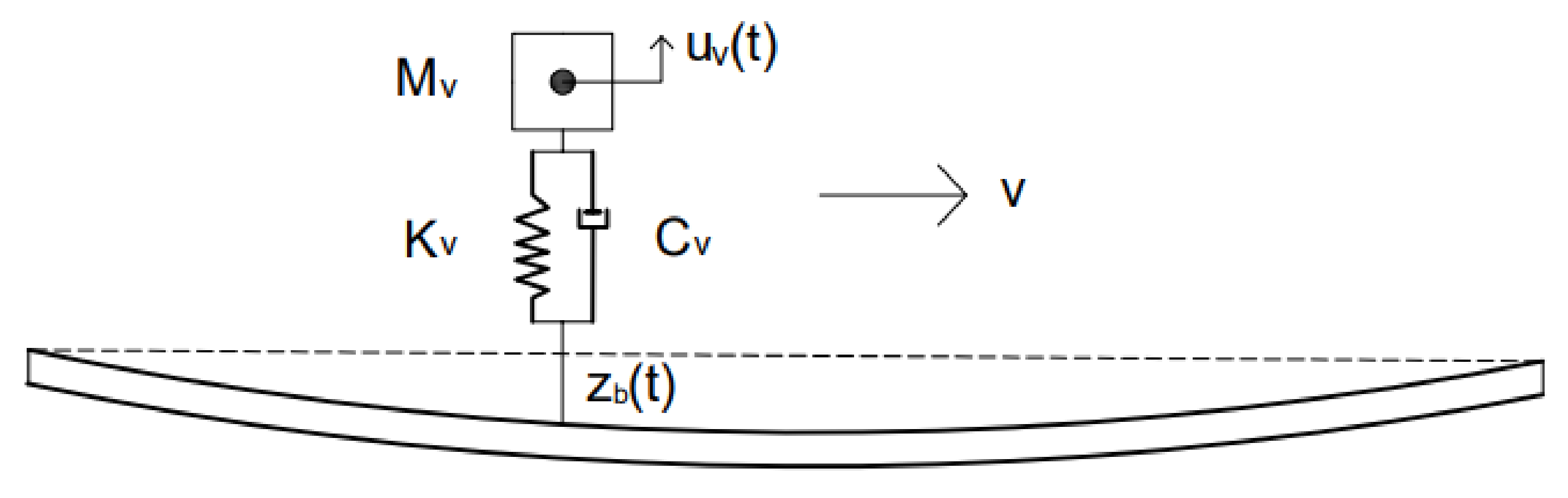
2.1. Theoretical Research on Vehicle–Axle Coupling Vibration

The whole mathematical model can be regarded as two subsystems; one is the vehicle subsystem and the other is the bridge subsystem. In the solution of vehicle–bridge coupling vibration equation [19], bridge mass, damping and stiffness matrices are generally constant matrices, bridge damping is selected as Rayleigh damping, and differential equations for bridge and vehicle vibration can be expressed as:

$$M_b{\ddot{Z}}_b\left(t\right)+C_b{\dot{Z}}_b\left(t\right)+K_b{Z}_b\left(t\right)=P_b\left(t\right)$$

(1)

where: $M_b$ is the bridge quality matrix, $C_b$ is the bridge damping matrix, $K_b$ is the bridge stiffness matrix, $Z_b$ is the bridge displacement matrix, ${\dot{Z}}_b$ is the bridge speed matrix, and ${\ddot{Z}}_b$ is the bridge acceleration matrix.

$$\left[M_v\right]\left\{{\ddot{u}}_v\left(t\right)\right\}+\left[C_v\right]\left\{{\dot{u}}_v\left(t\right)\right\}+\left[K_v\right]\left\{u_v\left(t\right)\right\}=\left\{P_v\left(t\right)\right\}$$

(2)

where $\left[M_v\right]$, $\left[C_v\right]$, and $\left[K_v\right]$ are vehicle generalized mass matrix, generalized damping matrix, and generalized stiffness matrix, respectively, $\left\{{\ddot{u}}_v\left(t\right)\right\}$, $\left\{{\dot{u}}_v\left(t\right)\right\}$, and $\left\{u_v\left(t\right)\right\}$ are vehicle acceleration vector, velocity vector, and displacement vector, respectively, and $\left\{P_v\left(t\right)\right\}$ is load vector.

In the vehicle–bridge coupling vibration system, the solution process of differential equation of vehicle–bridge vibration is based on the geometric compatibility and mutual constraint of force balance at the contact point between wheel and bridge surface, the force acting on the wheel is obtained by using the relative displacement between the axle, and the vehicle matrix operation is used to obtain the force of the vehicle on the bridge. The displacement of the wheel relative to the road surface can be expressed as:

$${\mathsf{\Delta }}_i=Z_{wi}-Z_i-r_i\left(x\right)$$

(3)

where $Z_{wi}$ is the vertical displacement of the wheel, $Z_i$ is the vertical displacement of the bridge at the contact point between the bridge and the wheel, and $r_i\left(x\right)$ is the pavement roughness at the bridge and point.

There is a pair of forces with equal size and opposite direction at the contact point between the wheel and the bridge. The gravity of the vehicle on the bridge should be considered in calculation and programming. The force balance can be expressed as:

$$F_{wi}=-F_{bi}=c_{wi}\left({\mathsf{\Delta }}_i^{\prime }\right)+k_{wi}\left({\mathsf{\Delta }}_i\right)$$

(4)

where $c_{wi}$ is wheel damping, $k_{wi}$ is the wheel stiffness, and ${\mathsf{\Delta }}_i$ is the vertical relative displacement between wheel and pavement.

The equation selects the Newmark-β method for solving the vehicle–bridge coupling system. The displacement and velocity of vehicles calculated by the Newmark-β method are used as the initial conditions for the next time interval to solve the vehicle–bridge coupling system. The differential equation of motion of the vehicle is:

$$\left[M\right]\left\{\ddot{u}\left(t\right)\right\}+\left[C\right]\left\{\dot{u}\left(t\right)\right\}+\left[K\right]\left\{u\left(t\right)\right\}=\left\{P\left(t\right)\right\}$$

(5)

where $\left\{\ddot{u}\right\}$ can be represented by linear acceleration interpolation, and $\left\{{\ddot{u}}_i\right\}$ can be represented by α control parameters, that is:

$$\left\{\ddot{u}\right\}=\left(1-\delta \right)\left\{{\ddot{u}}_i\right\}+\delta \left\{{\ddot{u}}_{i+1}\right\} \left(0\le \delta \le 1\right)$$

(6)

$$\left\{\ddot{u}\right\}=\left(1-2\alpha \right)\left\{{\ddot{u}}_i\right\}+2\alpha \left\{{\ddot{u}}_{i+1}\right\} \left(0\le \alpha \le \frac{1}{2}\right)$$

(7)

In turn, the structural acceleration vector and velocity vector at the $t_{i+1}$ moment can be derived:

$$\left\{{\ddot{u}}_{i+1}\right\}=a_0\left(\left\{u_{i+1}\right\}-\left\{u_i\right\}\right)-a_2\left\{{\dot{u}}_i\right\}-a_3\left\{{\ddot{u}}_i\right\}$$

(8)

$$\left\{{\dot{u}}_{i+1}\right\}=a_1\left(\left\{u_{i+1}\right\}-\left\{u_i\right\}\right)-a_4\left\{{\dot{u}}_i\right\}-a_5\left\{{\ddot{u}}_i\right\}$$

(9)

where $a_0=\frac{1}{\alpha \mathsf{\Delta }{t}^2}$; $a_1=\frac{\delta }{\alpha \mathsf{\Delta }t}$; $a_2=\frac{1}{\alpha \Delta t}$; $a_3=\frac{1}{2\alpha }-1$; $a_4=\frac{\delta }{\alpha }-1$; $a_5=\frac{\mathsf{\Delta }t}{2}\left(\frac{\delta }{\alpha }-2\right)$; $a_6=\mathsf{\Delta }t\left(1-\delta \right)$; $a_7=\delta \mathsf{\Delta }t$.

Then, the equation of motion of the structure at time $t_{i+1}$ can be written according to Equation (5):

$$\left[M\right]\left\{{\ddot{u}}_{i+1}\left(t\right)\right\}+\left[C\right]\left\{{\dot{u}}_{i+1}\left(t\right)\right\}+\left[K\right]\left\{u_{i+1}\left(t\right)\right\}=\left\{P_{i+1}\left(t\right)\right\}$$

(10)

Replace Equations (8) and (9) into Equation (10):

$$\left({\alpha }_0\left[M\right]+{\alpha }_1\left[C\right]+\left[K\right]\right)\left\{u_{i+1}\right\}=\left\{P_{i+1}\right\}+\left[M\right]\left(a_0\left\{u_i\right\}+a_2\left\{{\dot{u}}_i\right\}+a_3\left\{{\ddot{u}}_i\right\}\right)+\left[C\right]\left(a_1\left\{u_i\right\}+a_4\left\{{\dot{u}}_i\right\}+a_5\left\{{\ddot{u}}_i\right\}\right)$$

(11)

According to Equation (10), the structural displacement vector $\left\{u_{i+1}\right\}$ at $t_{i+1}$ time can be obtained by substituting the structural displacement vector $\left\{u_{i+1}\right\}$ into Equations (7) and (8) to obtain the structural acceleration vector $\left\{{\ddot{u}}_{i+1}\right\}$ and the structural velocity vector $\left\{{\dot{u}}_{i+1}\right\}$ at the $t_{i+1}$ time.

2.2. Theoretical Analysis of Detection Method Based on Vehicle Response

Indirect measurement of bridge damage using vehicle response begins with the bridge frequency indirect measurement method proposed by Yang and Chang et al., and the first-order frequency of the bridge can be identified by performing an FFT transformation on the acceleration response of the vehicle. Yang et al. derived the vehicle acceleration response [20]:

$${\ddot{q}}_v\left(t\right)={\displaystyle \sum }_{i=1}^n\left\{\begin{array}{c}{P}_{i}cos\left({\omega }_{v}t\right)+Q_{i}cos\left(2{\omega }_{ci}t\right)+\\ X_{i}cos\left[\left({\omega }_{ci}-{\omega }_i\right)t\right]+Y_{i}cos\left[\left({\omega }_{ci}+{\omega }_i\right)t\right]\end{array}\right\}$$

(12)

where $P_i$, $Q_i$, $X_i$, and $Y_i$ is a time-independent coefficient, ${\omega }_i$ is the i−th natural frequency of the bridge, ${\omega }_v$ is the natural vibration frequency of the vehicle, and ${\omega }_{ci}=i\pi v/L$ is the vehicle loading frequency.

The load vector $\left\{P_{i+1}\right\}$ at the right end of the vehicle vibration differential equation can be expressed by the bridge displacement and speed, and the load vector $\left\{P_{i+1}\right\}$ of 1/4 vehicle model is:

$$\left\{P_{i+1}\right\}=\left(\begin{array}{c}0\\ c_{w1}{f}_z^{\prime }\left(x\right)+k_{w1}{f}_z\left(x\right)\end{array}\right)$$

(13)

where $c_{w1}$ is wheel damping, $k_{w1}$ is the wheel stiffness, $f_z\left(x\right)$ is the bridge displacement, and $f_z^{\prime }\left(x\right)$ is the bridge speed.

With the tractor test truck model, both the tractor and the inspection vehicle can be reduced to a concentrated force compared to the bridge span, as shown in Figure 2.

The deflection at the position of the detection vehicle can be calculated using the superposition principle:

$$f_z\left(x\right)=\frac{F_c{x}^2{(x-l)}^2}{3EIl}+\frac{F_q}{EI}\cdot \left[-\frac{\left(l-\left(x+\mathsf{\Delta }a\right)\right)x^3}{6l}+\left(\frac{{(x+\mathsf{\Delta }a)}^3}{6l}+\frac{\left(x+\mathsf{\Delta }a\right)l}{3}-\frac{{(x+\mathsf{\Delta }a)}^2}{2}\right)x\right]$$

(14)

where $\mathsf{\Delta }a$ is the distance between the tractor and the center of mass of the test vehicle.

Replace Equations (13) and (14) into Formula (11) to detect the displacement vector of the vehicle at the driving position $\left\{u_{i+1}\right\}$:

$$\left\{u_{i+1}\right\}=\frac{1}{b_2{b}_1-b_3^2}\left[\begin{array}{c}{b}_1\left(b_4+b_6\right)+b_3\left(c_{w1}{f}_z^{\prime }\left(x\right)+k_{w1}{f}_z\left(x\right)+b_5+b_7\right)\\ b_3\left(b_4+b_6\right)+b_2\left(c_{w1}{f}_z^{\prime }\left(x\right)+k_{w1}{f}_z\left(x\right)+b_5+b_7\right)\end{array}\right]$$

(15)

where:

$$\begin{gathered} b_1=a_0{m}_{w1}+a_1\left(c_{u1}+c_{w1}\right)+\left(k_{u1}+k_{w1}\right) \\ {b}_2=a_0{m}_v+a_1{c}_{u1}+k_{u1} \\ {b}_3=a_1{c}_{u1}+k_{u1} \\ {b}_4=m_v\left(a_0{u}_{i1}+a_2{\dot{u}}_{i1}+a_3{\ddot{u}}_{i1}\right) \\ {b}_5=m_{w1}\left(a_0{u}_{i2}+a_2{\dot{u}}_{i2}+a_3{\ddot{u}}_{i2}\right) \\ {b}_6=c_{u1}\left(a_1{u}_{i1}+a_4{\dot{u}}_{i1}+a_5{\ddot{u}}_{i1}\right)-c_{u1}\left(a_1{u}_{i2}+a_4{\dot{u}}_{i2}+a_5{\ddot{u}}_{i2}\right) \\ {b}_7=\left(c_{u1}+c_{w1}\right)\left(a_1{u}_{i2}+a_4{\dot{u}}_{i2}+a_5{\ddot{u}}_{i2}\right)-c_{u1}\left(a_1{u}_{i1}+a_4{\dot{u}}_{i1}+a_5{\ddot{u}}_{i1}\right) \end{gathered}$$

(16)

Replace Equation (15) with Equation (8) to detect the acceleration vector of the car at the driving position $\left\{{\ddot{u}}_{i+1}\right\}$

$$\left\{{\ddot{u}}_{i+1}\right\}=\left[\begin{array}{c}\frac{a_0}{b_2{b}_1-b_3^2}\left(b_1\left(b_4+b_6\right)+b_3\left(\begin{array}{c}{c}_{w1}{f}_z^{\prime }\left(x\right)\\ +k_{w1}{f}_z\left(x\right)+b_5+b_7\end{array}\right)\right)-a_0{u}_{i1}-a_2{\dot{u}}_{i1}-a_3{\ddot{u}}_{i1}\\ \frac{a_0}{b_2{b}_1-b_3^2}\left(b_3\left(b_4+b_6\right)+b_2\left(\begin{array}{c}{c}_{w1}{f}_z^{\prime }\left(x\right)\\ +k_{w1}{f}_z\left(x\right)+b_5+b_7\end{array}\right)\right)-a_0{u}_{i2}-a_2{\dot{u}}_{i2}-a_3{\ddot{u}}_{i2}\end{array}\right]$$

(17)

The acceleration response of the car body is:

$$a_{v1}=\frac{a_0}{b_2{b}_1-b_3^2}\left(\begin{array}{c}{b}_1\left(b_4+b_6\right)+b_3(c_{w1}{f}_z^{\prime }\left(x\right)\\ +k_{w1}{f}_z\left(x\right)+b_5+b_7)\end{array}\right)-a_0{u}_{i1}-a_2{\dot{u}}_{i1}-a_3{\ddot{u}}_{i1}$$

(18)

When there is damage somewhere in the bridge and the bridge stiffness decreases, the deflection of the bridge at the damage location is:

$$f_{z{\theta }_d}=\frac{1}{1-{\theta }_d}\left\{\frac{F_q}{EI}\left[\begin{array}{c}\left(\frac{{\left(x+\mathsf{\Delta }a\right)}^3}{6l}+\frac{\left(x+\mathsf{\Delta }a\right)l}{3}-\frac{{\left(x+\mathsf{\Delta }a\right)}^2}{2}\right)x\\ -\frac{\left(l-\left(x+\mathsf{\Delta }a\right)x^3\right)}{6l}\end{array}\right]+\frac{F_c{x}^2{\left(x-l\right)}^2}{6l}\right\}=\frac{1}{1-{\theta }_d}{f}_z\left(x\right)$$

(19)

where ${\theta }_d$ is the degree of damage to the bridge.

The vehicle’s body acceleration response at the point of injury is:

$$a_{v1\theta }=\frac{a_0}{b_2{b}_1-b_3^2}\left(\begin{array}{c}{b}_1\left(b_4+b_6\right)+b_3(\frac{1}{1-{\theta }_d}{c}_{w1}{f}_z^{\prime }\left(x\right)\\ +\frac{1}{1-{\theta }_d}{k}_{w1}{f}_z\left(x\right)+b_5+b_7)\end{array}\right)-a_0{u}_{i1}-a_2{\dot{u}}_{i1}-a_3{\ddot{u}}_{i1}$$

(20)

From Equations (18) and (20), it can be seen that the acceleration response of the car body contains bridge deflection and speed response information, and the acceleration response of the car body through the bridge is processed and analyzed, and the bridge information can be identified. When a bridge is damaged, the deflection of the bridge changes accordingly at the location of the damage, and this change will be reflected in the acceleration response of the car body, so the damage location can be identified by using the acceleration response of the car body.

2.3. Wavelet Analysis

At the initial stage of structural damage or when the damage is relatively small, the changes of structural response caused by the damage are also very small. In order to highlight the damage information in vehicle response, wavelet analysis is applied in dynamic response signal analysis. As a new method in the field of signal processing, wavelet analysis can effectively identify the subtle differences in signals. It carries out multi-scale analysis on the signal in time domain and frequency domain, so that the signal can be time-refined at high frequency and frequency-refined at low frequency. Therefore, it is widely used in the field of signal detection.

Wavelet transforms are divided into continuous wavelet transforms and discrete wavelet transforms, continuous wavelet transform (CWT) can decompose the original signal into a two-dimensional signal; by adjusting the scale factor m and translation factor n, the original signal $f\left(s\right)$ is analyzed to obtain the signal local detection information. The original signal $f\left(s\right)$ is continuously transformed at the scale factor m and the translation factor n, because the adjustment factor has continuity, so the wavelet transformation coefficient will generate a large amount of redundant data, which is not conducive to signal processing, so a discrete wavelet transform (DWT) is introduced. The scale factor m and translation factor n are generally calculated as follows:

$$m=m_0^j$$

(21)

$$n=k{m}_0^j{n}_0$$

(22)

where $k$ and j are integers and $m_0\ne 1$.

The discrete wavelet transform function is:

$$W{T}_f\left(m,n\right)={\left|m_0\right|}^{-\frac{j}{2}}{{\displaystyle \int }}_{-\infty }^{+\infty }f\left(s\right){\varphi }^{*}{}_{m,n}\left(m_0^{-j}s-k{n}_0\right)ds$$

(23)

Discrete wavelet transform effectively reduces the redundant data generated by continuous wavelet transform and improves the calculation efficiency and accuracy. In this paper, discrete wavelet transform is used to analyze the vehicle dynamic response data and accurately find the subtle changes in the data, which is conducive to bridge damage identification.

2.4. Example Verification

In order to verify the accuracy of the program, the vehicle response spectrum obtained in this paper is compared with reference [7]. When the verification program is correct in this section, the same bridge and vehicle parameters as those in the literature are selected. The schematic diagram of the model is shown in Figure 1. The span diameter of the simple branch girder bridge was 25 m; cross-sectional area A = 2 m²; cross-sectional moment of inertia I = 0.12 m²; bridge elastic modulus E = 2.75 × 10¹⁰ N/m²; bridge unit length mass of 4800 kg/m; vehicle body mass $m_v$ = 1200 kg; wheel stiffness $k_w$ = 500,000 N/m; vehicle speed v = 10 m/s; other parameters of the vehicle were set to 0. The extracted acceleration response was used as a fast Fourier transform. The spectrum of acceleration response obtained is shown in in Figure 3.

It can be seen from Figure 3 that the extracted bridge frequency and vehicle frequency are 2.01 Hz and 3.22 Hz, respectively, which are very close to the bridge frequency and vehicle frequency of 2.08 Hz and 3.25 Hz in the literature. Input and output are the same, which proves the correctness of the program. This shows that the dynamic performance of the bridge can be identified and determined from the vehicle response.

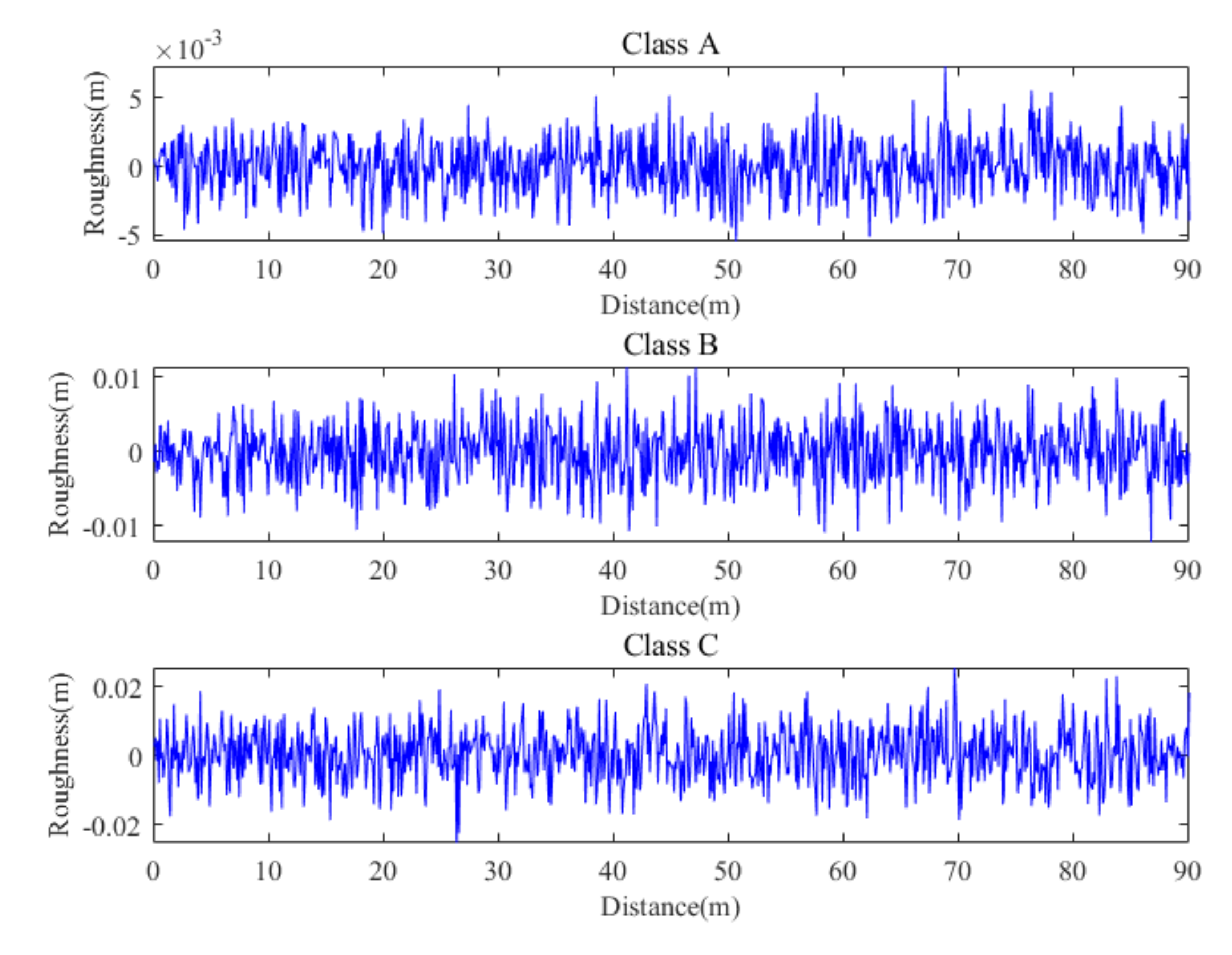
2.5. Influence of Road Roughness

In practical measurement, vehicle response is not only related to vehicle performance and bridge performance, but also related to road roughness. Additionally, uneven bridge deck is the main source of motivation that affects vehicle vibration, especially vertical vibration of vehicles [21], and naturally affects indirect detection methods based on vehicle response.

According to the mathematical definition, road surface irregularity is a random function, and the harmonic superposition method can simulate a stationary random process. The main idea is to express road roughness as the sum of a large number of sine and cosine functions with random phases. It has the characteristics of fast calculation speed and high accuracy. The road surface irregularity value at each position is calculated by the harmonic superposition method, and the calculation formula is as follows

$$r\left(x\right)={\displaystyle \sum }_{k=1}^N{\alpha }_{k}cos({\omega }_{k}x+{\phi }_k)$$

(24)

$${\alpha }_k=\sqrt{4G_d\left(n_k\right)\mathsf{\Delta }n}$$

(25)

$$n_k=n_1+\left(k-\frac{1}{2}\right)\mathsf{\Delta }n k=1, 2, \dots N$$

(26)

$$\mathsf{\Delta }n=\frac{n_2-n_1}{N}$$

(27)

In the formula: $r\left(x\right)$ is the uneven sample waveform; ${\omega }_k$ is the circular frequency, with a value of $2\pi n_k$; ${\phi }_k$ is a random phase angle, with a value between $\left[0, 2\pi \right]$; N is a sufficiently large integer, which is an equal fraction of the spatial frequency; and $G_d\left(n\right)$ is the pavement power spectrum function.

The harmonic superposition method is used to simulate road irregularity, and MATLAB software is used to simulate the irregularity sample functions of three pavement grades A–C, as shown in Figure 4.

It can be seen from Figure 4 that the pavement irregularity value increases with the decrease in pavement grade. The peak irregularity values of three pavement grades A–C are 5.78 mm, 11.49 mm, and 27.86 mm, respectively.

3. Identification of Bridge Damage Location under the Action of Mobile Vehicles

3.1. Theoretical Basis

Before the bridge is put into use and in normal operation, many experiments are carried out to observe its performance. In this chapter, combined with the vehicle–bridge coupling vibration analysis algorithm mentioned above, considering the influence of road roughness, an indirect measurement method based on health data is proposed. The vehicle response when the detection vehicle passes through the damaged bridge is compared with the vehicle response data when the bridge is in a healthy state. The acceleration responses of the two vehicles are subtracted; then, the acceleration response difference is transformed by wavelet transform, and the bridge damage location is located through the peak value of wavelet transform.

By subtracting Equations (18) and (20), the acceleration response difference in the vehicle body can be obtained:

$$\mathsf{\Delta }{a}_{v\theta }\left(x\right)=\left\{\begin{array}{c}H\left(x\right)\\ \frac{a_0{b}_3}{b_2{b}_1-b_3^2}\left(c_{w1}{f}_z^{\prime }\left(x\right)+k_{w1}{f}_z\left(x\right)\right)\cdot \frac{{\theta }_d}{1-{\theta }_d}+H\left(x\right)\end{array}\begin{array}{c}Undamaged location\\ Damage location\end{array}\right.$$

(28)

where:

$$H\left(x\right)=a_0{u}_{i11}+a_2{\dot{u}}_{i11}+a_3{\ddot{u}}_{i11}-a_0{u}_{i12}-a_2{\dot{u}}_{i12}-a_3{\ddot{u}}_{i12}+\frac{a_0}{b_2{b}_1-b_3^2}\left(\begin{array}{c}{b}_1\left(b_{42}+b_{62}-b_{41}-b_{61}\right)\\ +b_{52}+b_{72}-b_{51}-b_{71}\end{array}\right)$$

(29)

It can be seen from Equation (28) that the acceleration response difference in the vehicle body has a large sudden change at the damage position, but the sudden change point cannot be identified on the acceleration response difference curve of the vehicle body. The damage position of the continuous beam bridge can be identified by discrete wavelet transform of the acceleration response difference in the vehicle body.

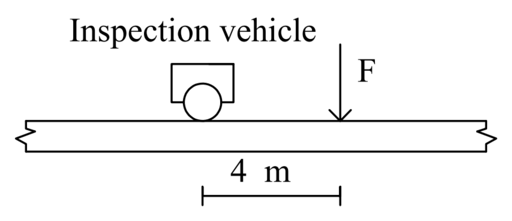
3.2. Model Establishment and Simplification

Taking the three-span continuous beam bridge with equal sections as an example, the total length of the bridge is 90 m, the span combination is 30 m + 30 m + 30 m, the bridge section height is 0.5 m, the bridge width is 3 m, the bridge elastic modulus E = 3 × 10¹⁰ N/m², and the mass per unit length of the bridge is 3300 kg/m. The beam3 element is used to simulate the bridge element, the division accuracy is 0.1 m, and the bridge damping adopts Rayleigh damping. The vehicle model adopts the tractor test vehicle model in the literature [20]; the acceleration sensor is placed at the centroid of the detection vehicle body, and there is no torque transmission between the two parts connecting the tractor and the detection vehicle. The tractor is only used as a provider of forward power of the detection vehicle, therefore there is no torque transmission between the tractor and the detection vehicle, so the tractor is simplified as a concentrated force acting on the center of mass of the tractor, as shown in Figure 5. The vehicle model is symmetrical left and right, so the detection vehicle model uses a 1/2 model for simplified calculation, and the tractor concentration force is 5880 N.

Vehicle parameters are set according to the actual vehicle parameters and documents [22,23], as shown in

Table 1. Vehicle parameters of the test vehicle.

Properties	Symbol	Unit	Value
Body mass	$m_v$	kg	2000
Car suspension and wheel mass	$m_{wi}$ (i = 1.2)	kg	100
Stiffness coefficient of vehicle suspension	$k_{ui}$ (i = 1.2)	N/m	4.07 × 105
Vehicle suspension damping coefficient	$c_{ui}$ (i = 1.2)	N·s/m	7509
Wheel stiffness coefficient	$k_{wi}$ (i = 1.2)	N/m	1.56 × 105
Wheel damping coefficient	$c_{wi}$ (i = 1.2)	N·s/m	1000
The lateral distance between the wheel and the center of mass of the car body	$d_i$ (i = 1.2)	m	1

.

3.3. Bridge Damage Conditions

In this paper, the bridge damage unit is simulated by using the stiffness reduction in the bridge damage area, and the damage degree is expressed by ${\theta }_d$. Six working conditions are preliminarily assumed, and the damage position x is the distance between the damage center point and the left end of the continuous girder bridge, as shown in the bridge damage condition

Table 2. Bridge damage conditions.

Working Condition Description	Serial Number	Damage Distance (x/m)	Degree of Damage (θd/%)
No damage	Working condition 1	\	0
Single damage	Working condition 2	5	20
	Working condition 3	20	30
	Working condition 4	45	20
Multiple damage	Working condition 5	20	30
		45	20
	Working condition 6	15	10
		45	20
		75	40

.

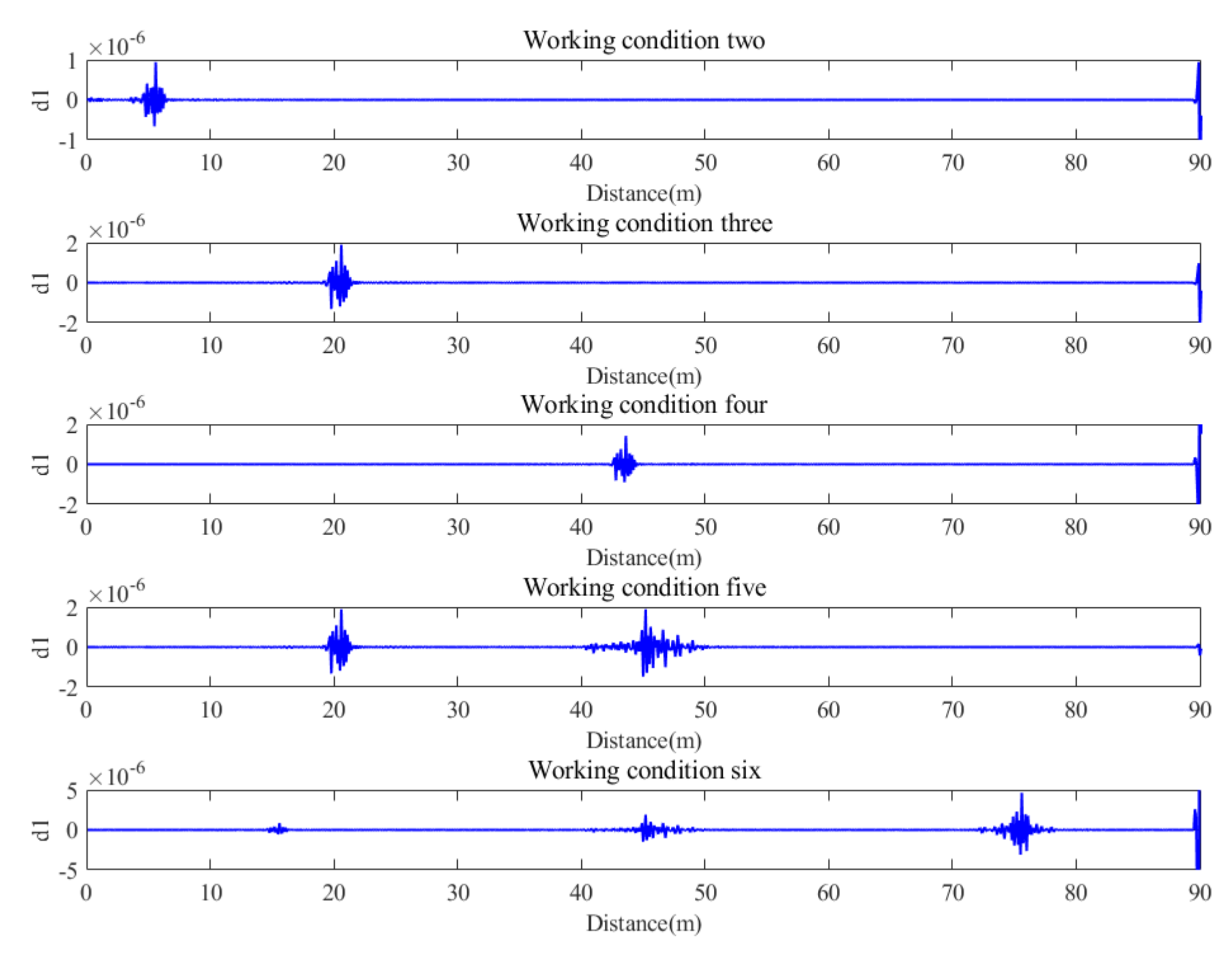
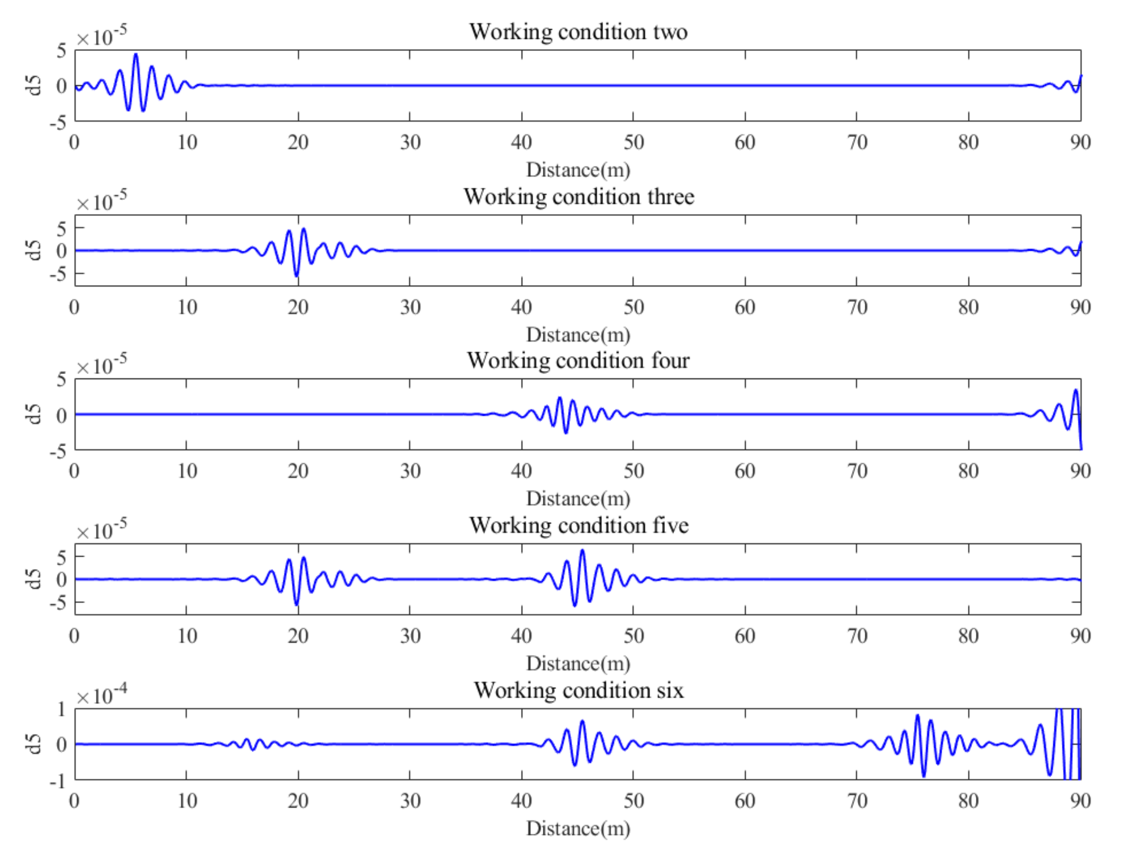
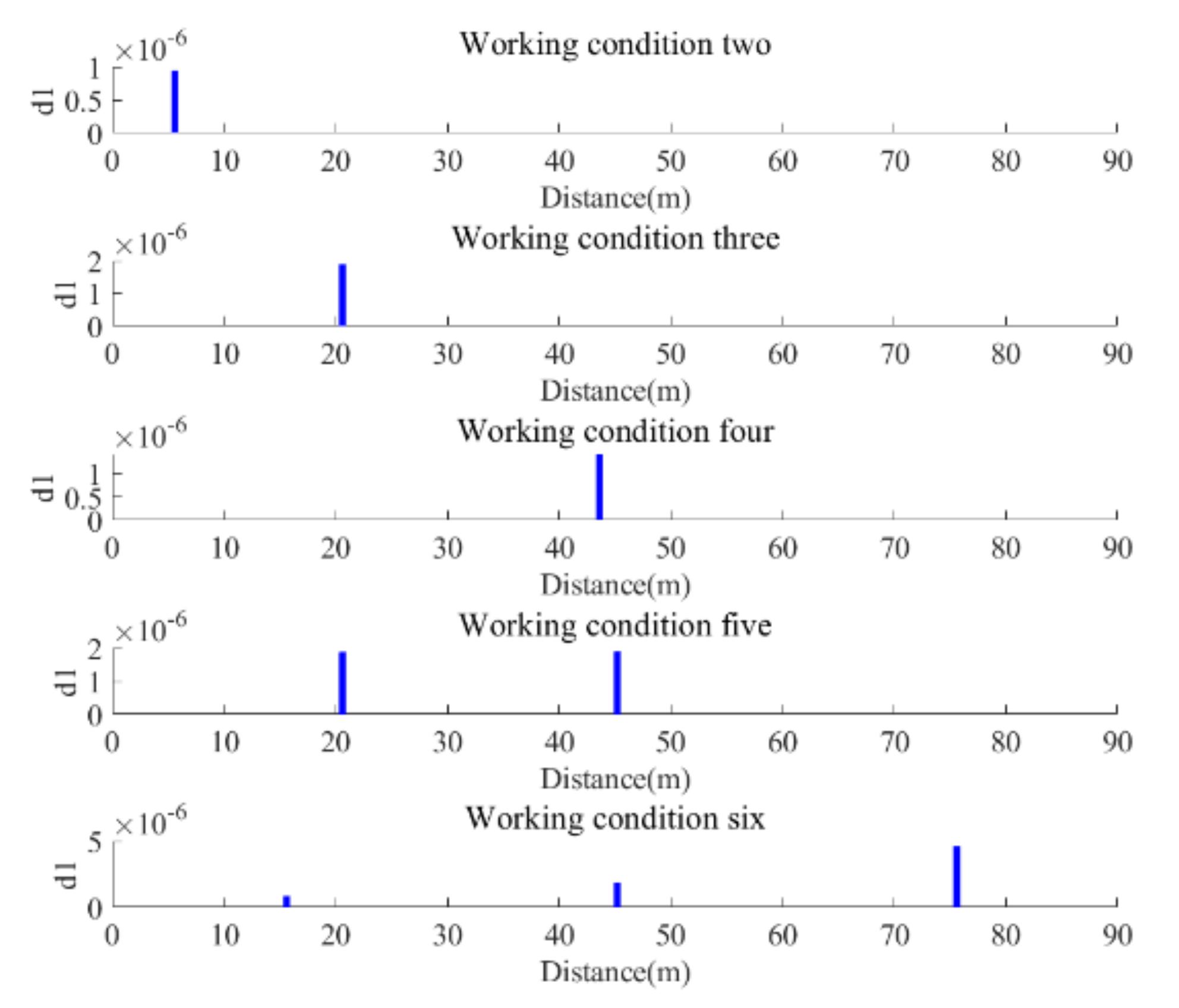
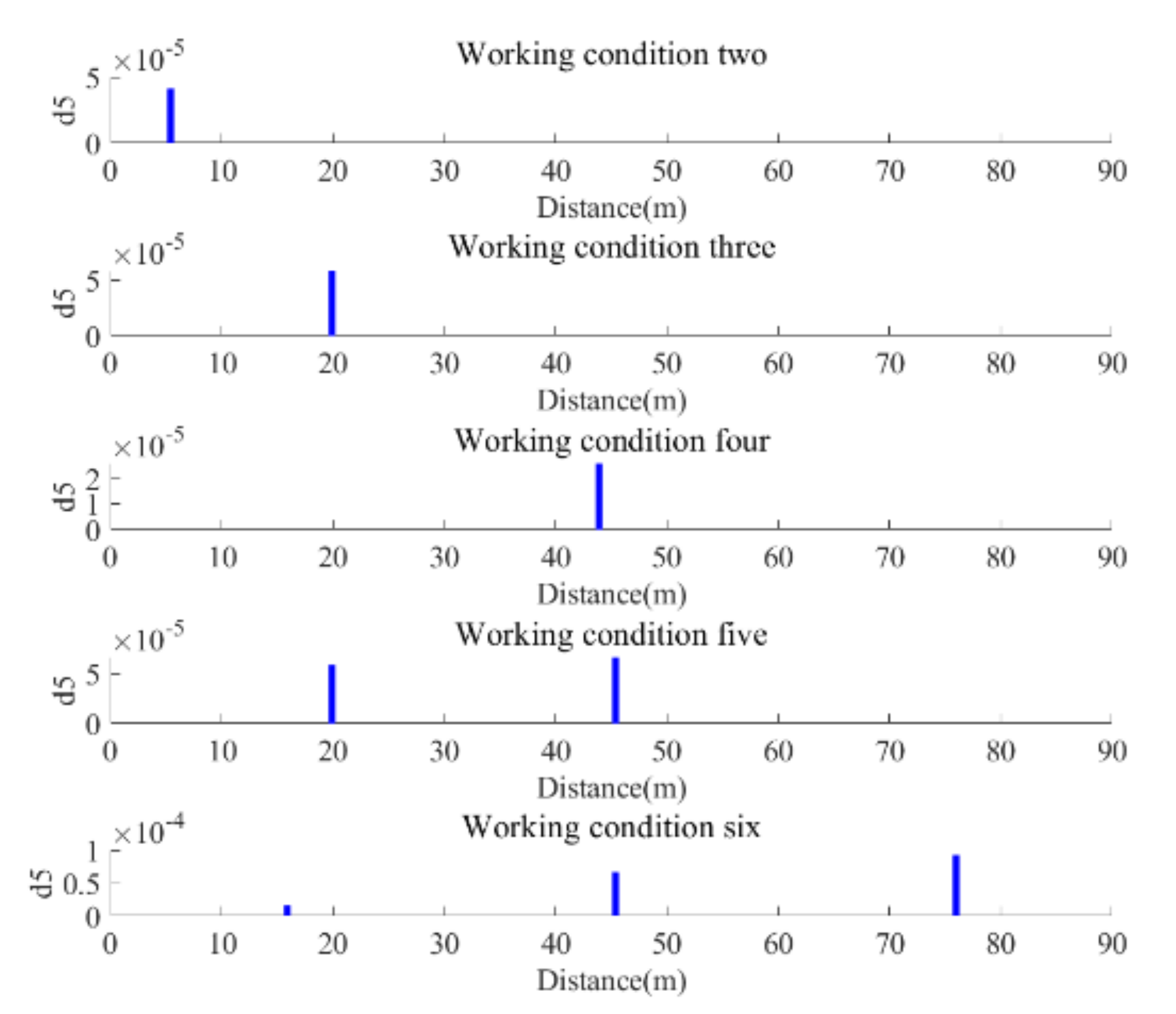
3.4. Identification of the Damage Location

For some new bridges, there are generally baseline data of the bridge’s intact condition. The bridge damage detection method based on bridge health data mainly collects the vertical acceleration response of the car body before and after the damage, and performs discrete wavelet transformation on the acceleration response difference in the car body before and after the bridge damage to identify the damage location. A simplified model is used for calculation in this section. The vehicle driving speed is 72 km/h, the road surface is uneven using Class A pavement, and the above damage conditions are simulated and calculated by using finite element software.

The wavelet basis function selects the bior4.4 wavelet and db20 wavelet for discrete wavelet transformation, and the d1 coefficient in the bior4.4 wavelet transform and the d5 coefficient in the db20 wavelet is selected to determine the damage position, and the damage position recognition of the working conditions 2–6 is shown in Figure 6 and Figure 7.

It can be seen from the wavelet variation coefficients in Figure 8 and Figure 9 that both wavelet coefficients have obvious sudden changes near the damage location. However, there is some interference near the damage location, which is not conducive to the accurate identification of the damage location and is easy to cause misjudgment. However, through the maximum successful approximation approach (MSAA) processing on the wavelet transform coefficients, the damage location can be accurately identified and misjudgment can be reduced. Figure 8 and Figure 9 shows the wavelet coefficients after the maximum successive approximation processing.

It can be seen from Figure 8 and Figure 9 that the wavelet transform coefficient of the acceleration response difference in the detection vehicle has a large mutation at the damage position, and the damage position can be determined. Using MSAA method to process wavelet coefficients can accurately locate the damage location and reduce misjudgment. Under the finite element simulation calculation, the bridge damage detection method based on health data can accurately locate the single damage and multiple damage of a continuous beam bridge. In condition 6, it can be seen that the peak value of wavelet transform coefficient increases with the increase in damage degree.

4. Influence Factors on Damage Location Identification

Bridge damage identification based on vehicle response involves vehicle parameters, bridge parameters, noise, and other factors, which will have a certain impact on bridge damage identification. Therefore, studying the influence of various factors on bridge damage identification will help to accurately locate bridge damage and select parameters. The following mainly studies the influence of vehicle weight, vehicle speed, road roughness, noise, and other factors on the damage location identification of a continuous beam bridge.

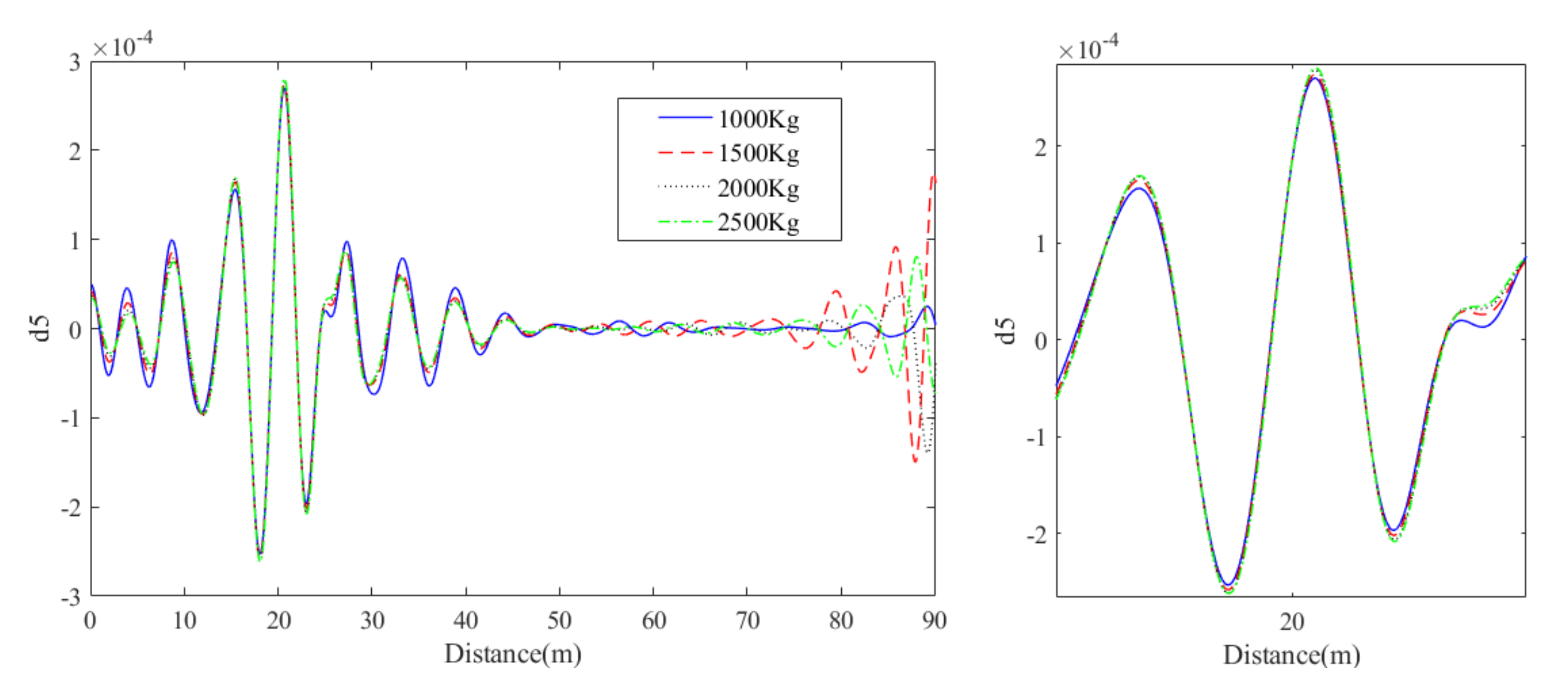
4.1. Influence of Vehicle Weight on Damage Location Identification

The weight of the inspection vehicle is an important parameter affecting vehicle response and bridge response. Considering the actual vehicle situation, the weight of the inspection vehicle was calculated by taking 1000 kg, 1500 kg, 2000 kg, and 2500 kg, respectively. Other vehicle parameters and bridge parameters were set according to Section 3.2. In order to study the influence of vehicle weight on damage recognition, we selected condition 3 in Section 3.3 (single damage; damage location: 20 m; damage degree: 30%) for calculation, and conducted discrete wavelet transform on the acceleration response difference in the vehicle body for bridge damage identification. The wavelet transform coefficients under different vehicle weights are shown in Figure 10.

As can be seen from Figure 10, with the increase in vehicle weight, the bridge damage can still be accurately identified by using the wavelet transform coefficient of vehicle acceleration difference, but the coefficient peaks of different vehicle weights are slightly different at the damage location. At the same time, when the vehicle weight exceeds 1000 kg, there is more interference in the wavelet transform coefficient near 90 m, which is not conducive to the location of bridge damage. According to the finite element simulation calculation results, the vehicle weight of the test vehicle shall be 1000 kg as far as possible.

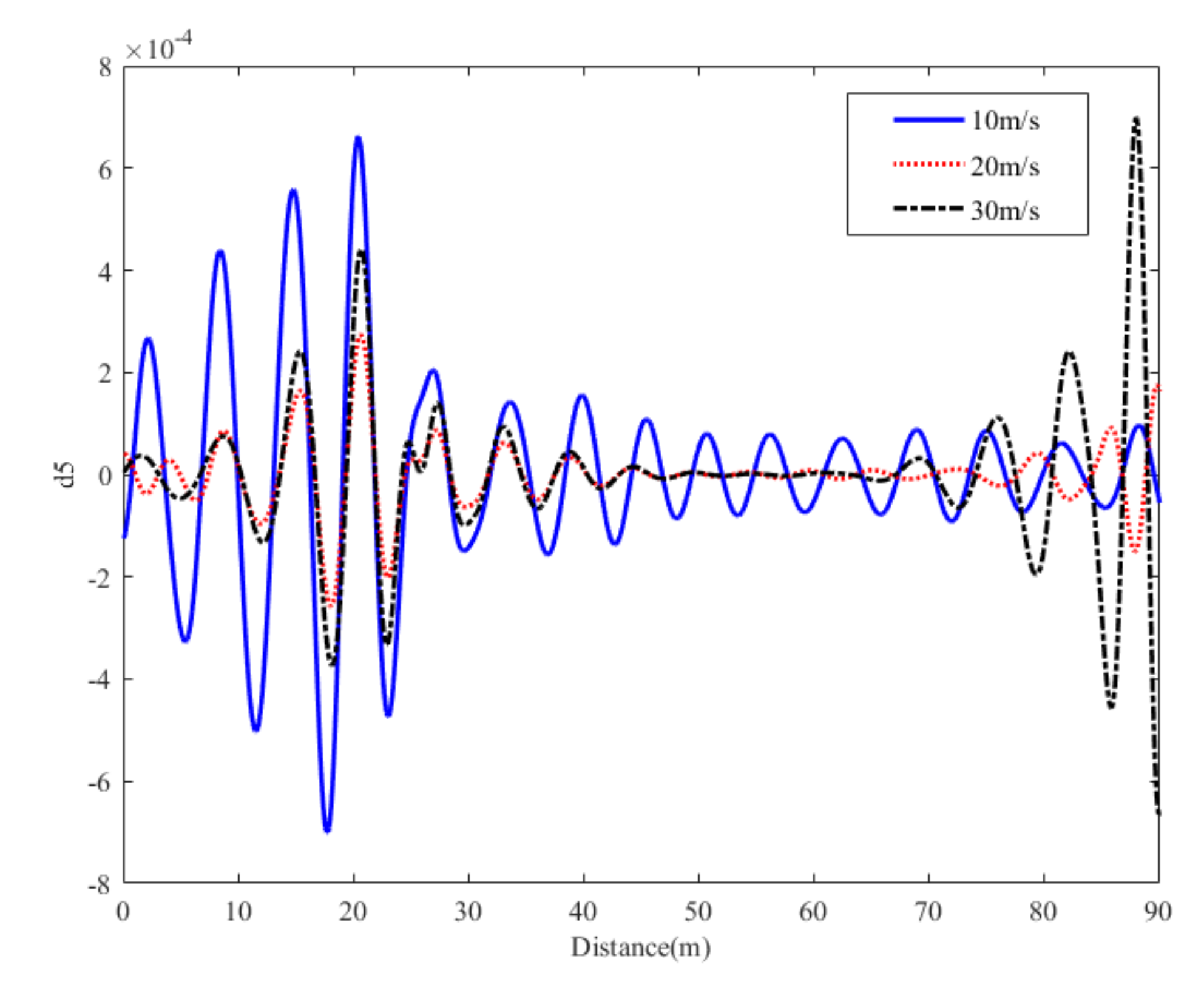
4.2. Influence of Vehicle Speed on Damage Location Identification

The change of the vehicle excitation frequency will affect the dynamic response of the vehicle–bridge coupling system. Naturally, it will have a certain impact on the bridge damage identification. When the vehicle speed is within a specific range, the vehicle acceleration signal changes drastically, and the wavelet transform coefficient peak value is obvious, which is beneficial to the location of bridge damage. The inspection vehicle weighed 1000 kg. The parameters of other vehicles and bridges remain unchanged, and the vehicle speeds were calculated as 10 m/s, 20 m/s, and 30 m/s, respectively, to study the influence of the speed change of the detected vehicle on the bridge damage identification. Working condition 3 in Section 3.3 (single damage; damage location: 20 m; damage degree 30%) was selected for calculation, and discrete wavelet transform was performed on the difference in acceleration response of the vehicle body to perform bridge damage identification, as shown in Figure 11.

When the vehicle speed is 10 m/s, 20 m/s, and 30 m/s, the damage can be accurately identified, and as the vehicle speed increases, the wavelet transform peak value first decreases and then increases. In theory, the test vehicle can travel at a speed of 10–30 m/s. However, if the sampling rate of the sensor is considered, it is required to collect enough sampling signals in a single test run; therefore, it is suggested that the speed should not be too high; when the speed is at 20 m/s and 30 m/s, the wavelet coefficients near the support will affect the damage identification. In addition, if the speed is too low it will lead to insufficient bridge excitation. Considering detection speed and detection effect, a vehicle speed of 10 m/s is recommended in this article.

4.3. Influence of Road Surface Roughness on Damage Identification

During on-site inspection, the uneven road surface will inevitably have a greater impact on the response of the vehicle, thereby affecting the identification of the bridge damage’s location. Using random simulation in Section 2.5 to generate grade A–C road roughness class, the impact of road irregularities on bridge damage identification was studied. The working condition 3 in Section 3.3 (single damage; damage location: 20 m; damage degree 30%) was selected for calculation, and discrete wavelet transform was performed on the difference in acceleration response of the vehicle body to perform bridge damage identification, as shown in Figure 12.

Analyzing Figure 12, it can be obtained that the damage location of bridge can be accurately identified under different road surface roughness, which shows that the road surface roughness has little influence on the bridge damage identification method. Under ideal road conditions, the use of acceleration response difference can effectively reduce the impact of roughness on the damage results, but it cannot be completely eliminated.

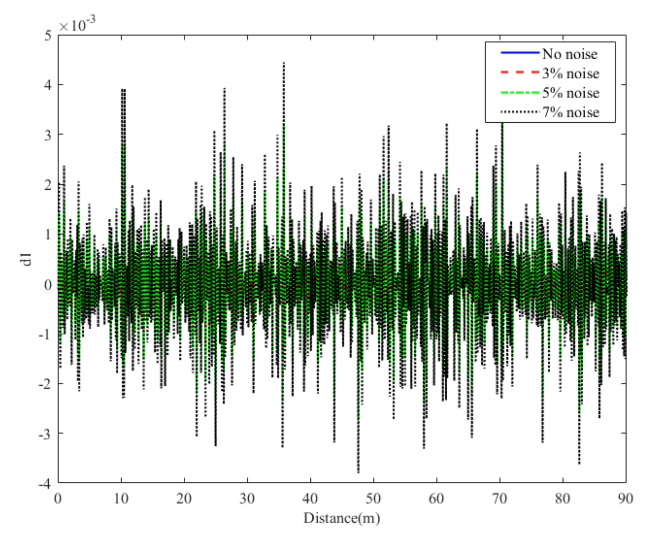
4.4. Influence of Noise on Damage Identification

During the on-site measurement and inspection process, due to the influence of the measurement environment and the measurement system, noise is inevitable, and the noise will “contaminate” the measurement data, which will have a greater impact on the later data processing and analysis. In order to study the effect of noise on the damage recognition effect of the method, white noise was superimposed on the acceleration response of the vehicle body, and the expression is as follows:

$$a_n=a+E_n{N}_{oise}\sigma \left(a\right)$$

(30)

where $a_n$ is the acceleration response with noise, a is the original acceleration response, $E_n$ is the noise level, $N_{oise}$ is the noise obeying the standard normal distribution N (0, 1), and $\sigma \left(a\right)$ is the standard deviation of the original acceleration response.

The noise level was 3%, 5%, and 7% in sequence, and the above Section 3.3 working condition 3 (single damage; damage location: 20 m; damage degree 30%) was selected as the damage condition, and the damage identification of the bridge by noise was studied. The influence of this is shown in Figure 13 and Figure 14.

When the sensor records the acceleration of the vehicle body, it will inevitably be affected by environmental noise. The frequency and energy of these noises will affect the wavelet transform, which may cause the results of the wavelet transform to be irregular, and the damage location cannot be identified. It can be seen from Figure 14 that when selecting the low-frequency area (d5) for damage identification, the wavelet transform coefficients under different levels of noise are basically the same as those under noise-free conditions, indicating that selecting the d5 coefficient for damage location identification has good anti-noise qualities. It can be seen from Figure 13 that when the high-frequency area (d1) is selected for damage identification, it cannot be identified at all in the presence of noise, and the amplitude of the wavelet coefficient increases with the increase in the noise level. This is mainly because the high-frequency energy of noise is higher than the low-frequency energy, which affects the damage identification of wavelet transform coefficients in the high-frequency region. However, the original signal can be denoised. The original signal is first decomposed in multiple layers, high-frequency coefficients are thresholded, and low-frequency coefficients are retained. Then, the signal is reconstructed through wavelet inverse transform to reduce the influence of noise on damage identification.

5. Judgment of Damage Degree of Continuous Beam Bridge

In bridge damage identification, it is not only necessary to identify the location of the bridge damage, but also to determine the degree of damage. This section will be based on the bridge deflection and deflection difference to judge the damage degree of the bridge.

5.1. Damage Index

The MSAA coefficient is used as the coefficient peak value of the wavelet transform coefficient at the damage position. By processing the MSAA coefficient, the damage degree index can be obtained. Compared with the low frequency coefficient (d5), the high frequency coefficient (d1) has more concentrated energy, and the MSAA coefficient peak value changes more regularly. Therefore, the bridge detection method based on bridge health data selects the bior4.4-d1 coefficient to determine the degree of damage.

The MSAA coefficient is the peak coefficient of the damage location obtained after the discrete wavelet transformation of the vehicle body acceleration response difference. Therefore, the MSAA coefficient is closely related to the vehicle body acceleration response difference. It can be seen from Equation (28) that the sudden change point of the vehicle body acceleration response difference at the damage location is mainly related to the healthy bridge deflection $f_z\left(x\right)$, so the MSAA coefficient at the damage location is divided by the healthy bridge deflection $f_z\left(x_{{\theta }_d}\right)$ at the same location. The $D_1$ coefficient of continuous beam bridge damage detection method based on bridge health data is:

$$D_1=\frac{w_m}{f_z\left(x_{{\theta }_d}\right)}$$

(31)

$$f_z\left(x_{{\theta }_d}\right)=\frac{F_q}{EI}\cdot \left[\begin{array}{c}-\frac{\left(l-\left(x_{{\theta }_d}+\mathsf{\Delta }a\right)\right)x_{{\theta }_d}{}^3}{6l}\\ +\left(\frac{{(x_{{\theta }_d}+\mathsf{\Delta }a)}^3}{6l}+\frac{\left(x_{{\theta }_d}+\mathsf{\Delta }a\right)l}{3}-\frac{{(x_{{\theta }_d}+\mathsf{\Delta }a)}^2}{2}\right)x_{{\theta }_d}\end{array}\right]+\frac{F_c{x}_{{\theta }_d}{}^2{(x_{{\theta }_d}-l)}^2}{3EIl}$$

(32)

where $w_m$ is the MSAA coefficient at the damage location, $f_z\left(x_{{\theta }_d}\right)$ is the healthy bridge deflection value at the damage location, and $x_{{\theta }_d}$ is the distance from the damage location to the left end of the span.

The MSAA coefficients of the same degree of damage vary greatly in different positions. The change trend in MSAA coefficient is similar to that of healthy bridge deflection. Under the same damage degree, the MASS coefficient of the mid span is the largest, and it gradually decreases from the middle of the span to the support, approximately in the shape of a parabola. Therefore, damage location adjustment factor $D_2$ should be introduced, so that the damage degree index of each position of the same damage degree is kept within a certain range as in Formula (33)

$$D_2=x_d{}^{0.5}$$

(33)

where $x_d$ is the distance between the damage location and the nearest support of the span, $x_{e1}$ is the distance between the damage location and the left end of the span, $x_{e2}$ is the distance between the damage location of the side span and the nearest bridge end, and $l_b$ is the length of the side span.

From Formulas (27) and (29), the damage degree index D of the continuous beam bridge damage detection method based on bridge health data is:

$$D=D_1\cdot D_2=\frac{w_m}{f_z\left(x_{{\theta }_d}\right)}\cdot x_d{}^{0.5}$$

(34)

The MSAA coefficient of the same damage position increases as the damage degree increases, and the change trend is in the form of a power function. Multiple damage degree indicators at a certain point of the bridge are used to fit the damage degree function $S\left(x\right)$, and the damage degree function $S_{d1}\left(x\right)$. Multiple damage degree indexes at 20 m from the damage position are selected for fitting, and the damage degree is 10%, 20%, 30%, 40%, 50%, and Matlab is selected for function fitting. Substituting the damage degree index D into the damage degree function $S\left(x\right)$, the damage degree function $S_{d1}\left(D\right)$ is expressed as:

$$S_{d1}\left(D\right)=10.49\times D^{0.4519}-0.1707$$

(35)

where D is an index of the degree of damage.

5.2. Judgment of Bridge Damage Degree Based on Health Data

Corresponding data processing was performed on the MSAA coefficients of each bridge damage condition in Table 2 to obtain the damage degree index D. Substituting the damage degree index D into the damage degree function $S_{d1}\left(D\right)$, the bridge damage degree can be determined, as shown in

Table 3. Judgment of Bridge Damage Degree.

Damage Conditions	Damage Position (x/m)	Degree of Damage (θd/%)	MSAA Coefficient	Damage Index D	Degree of Damage (Sd1(D)/%)	Judgment Error (Rd/%)
Working condition 2	5	20	9.44 × 10−7	4.57 × 10−4	18.17	−1.83
Working condition 3	20	30	1.89 × 10−6	9.06 × 10−4	29.95	−0.05
Working condition 4	43	20	1.42 × 10−6	4.86 × 10−4	19.08	−0.92
Working condition 5	20	30	1.80 × 10−6	9.08 × 10−4	29.99	−0.01
	45	20	1.89 × 10−6	4.90 × 10−4	19.21	−0.79
Working condition 6	15	10	8.55 × 10−7	2.56 × 10−4	10.71	0.71
	45	20	1.90 × 10−6	4.85 × 10−4	19.06	−0.94
	75	40	4.64 × 10−6	1.43 × 10−3	40.07	0.07

.

It can be seen from Table 3 that the above-mentioned data processing method can be used to determine the degree of damage at each position of the bridge, with a maximum error of 2.81%, which is relatively small. The bridge damage degree determination is based on the MSAA coefficient through data fitting, and the MSAA coefficient is derived from the wavelet transform coefficient, so the accuracy of the damage degree determination is also affected by environmental noise, sensor accuracy, and road surface roughness.

6. Conclusions

(1)

Using the maximum value successive approximation method to process the wavelet transform coefficient can accurately identify the damage location, and the identification accuracy is affected by vehicle speed, vehicle weight, road surface roughness, and noise. The recommended speed is 10 m/s, and the recommended vehicle weight is 1000 kg.

(2)

This damage detection method has good noise immunity. The vehicle response signal needs to be processed by wavelet noise reduction when the noise is greater. When the noise level is not higher than 5%, the location of the bridge damage can be identified successfully.

(3)

The corresponding damage degree index D and the damage degree function $S_{d1}\left(D\right)$ are put forward. According to this, the damage degree of the bridge can be judged, and the judgment error of the damage degree basically meets the requirements, which is suitable for continuous beam bridges with different span combinations.

References

1. Chen, Q. Wuyishan Gongguan Bridge with a “Tragic Fate”. China Safety Production News N, 19 July 2011. [Google Scholar]
2. Zadehmohamad, M.; Bazaz, J.B.; Riahipour, R.; Farhangi, V. Physical modeling of the long-term behavior of integral abutment bridge backfill reinforced with tire-rubber. Int. J. Geo-Eng. 2021, 12, 36. [Google Scholar] [CrossRef]
3. Bandara, R.P.; Chan, T.; Thambiratnam, D. Structural damage detection method using frequency response functions. Struct. Health Monit. 2014, 13, 418–429. [Google Scholar] [CrossRef]
4. Zhan, J.; Xia, H.; Zhang, N. Bridge damage identification method based on online vibration response. China Railw. Sci. 2011, 32, 58–62. [Google Scholar]
5. Zhao, H. Performance Monitoring and Evaluation of Long-Span Cable-Stayed Bridges during Operation Period. Ph.D. Thesis, Southwest Jiaotong University, Chengdu, China, 2015. [Google Scholar]
6. Yang, Y.-B.; Lin, C.; Yau, J. Extracting bridge frequencies from the dynamic response of a passing vehicle. J. Sound Vib. 2004, 272, 471–493. [Google Scholar] [CrossRef]
7. Yang, Y.-B.; Lin, C. Vehicle–bridge interaction dynamics and potential applications. J. Sound Vib. 2005, 284, 205–226. [Google Scholar] [CrossRef]
8. Bu, J.Q.; Law, S.S.; Zhu, X.Q. Innovative Bridge Condition Assessment from Dynamic Response of a Passing Vehicle. J. Eng. Mech. 2006, 132, 1372–1379. [Google Scholar] [CrossRef]
9. Nguyen, K.V.; Tran, H.T. Multi-cracks detection of a beam-like structure based on the on-vehicle vibration signal and wavelet analysis. J. Sound Vib. 2010, 329, 4455–4465. [Google Scholar] [CrossRef]
10. Sun, Z.; Zhang, Y.; Tong, S. Summary of Bridge Damage Detection Methods Based on Vehicle-Bridge Coupling Vibration. World Earthq. Eng. 2013, 29, 1–8. [Google Scholar]
11. Yang, Y.-B.; Li, Y.; Chang, K. Constructing the mode shapes of a bridge from a passing vehicle: A theoretical study. Smart Struct. Syst. 2014, 13, 797–819. [Google Scholar] [CrossRef]
12. Malekjafarian, A.; Obrien, E. Identification of bridge mode shapes using Short Time Frequency Domain Decomposition of the responses measured in a passing vehicle. Eng. Struct. 2014, 81, 386–397. [Google Scholar] [CrossRef] [Green Version]
13. Obrien, E.J.; Malekjafarian, A.; González, A. Application of empirical mode decomposition to drive-by bridge damage detection. Eur. J. Mech. A/Solids 2017, 61, 151–163. [Google Scholar] [CrossRef] [Green Version]
14. Qian, Y. Bridge Frequency Identification and Damage Detection Based on Indirect Measurement Method. Master’s Thesis, Chongqing University, Chongqing, China, 2018. [Google Scholar]
15. Marashi, S.M.; Pashaei, M.H.; Khatibi, M.M. Estimating the Mode Shapes of a Bridge Using Short Time Transmissibility Measurement from a Passing Vehicle. Appl. Comput. Mech. 2019, 5, 735–748. [Google Scholar]
16. Locke, W.; Sybrand, J.; Redmond, L.; Safro, I.; Atamturktur, S. Using Drive-by health monitoring to detect bridge damage considering environmental and operational effects. J. Sound Vib. 2020, 468, 115088. [Google Scholar] [CrossRef]
17. Clemente, P.; Bongiovanni, G.; Buffarini, G.; Saitta, F. Structural health status assessment of a cable-stayed bridge by means of experimental vibration analysi. J. Civ. Struct. Health Monit. 2019, 9, 655–669. [Google Scholar] [CrossRef]
18. Farhangi, V.; Karakouzian, M. Design of Bridge Foundations Using Reinforced Micropiles. In Proceedings of the International Road Federation Global R2T Conference & Expo, Las Vegas, NV, USA, 19–22 November 2019. [Google Scholar]
19. Zhao, L. Vehicle-Bridge Coupling Vibration Analysis of Long-span Highway Concrete Filled Steel Tube Arch Bridge. Master’s Thesis, Zhengzhou University, Zhengzhou, China, 2017. [Google Scholar]
20. Lin, C.; Yang, Y.-B. Use of a passing vehicle to scan the fundamental bridge frequencies: An experimental verification. Eng. Struct. 2005, 27, 1865–1878. [Google Scholar] [CrossRef]
21. Han, W.; Ma, L.; Yuan, S.; Zhao, S. Analysis of the influence of non-uniform excitation of road surface roughness on the response of vehicle-bridge coupled vibration system. China Civ. Eng. J. 2011, 44, 81–90. [Google Scholar]
22. Guo, X.; Peng, M.; Zou, J.; Zhang, J.; Zhang, H. Research on Influencing Factors of Energy Feedback Potential of Commercial Vehicle Suspension. Chin. J. Highw. Transp. 2016, 29, 151–158. [Google Scholar]
23. Yao, C. Analysis and Research on Road Vehicle-Bridge Coupling Vibration Considering the Influence of Bridge Surface Irregularities. Master’s Thesis, Central South University, Changsha, China, 2011. [Google Scholar]
Figure 1. Mathematical model for vehicle scanning method.
Applsci 12 03743 g001
Figure 2. Schematic diagram of simplified calculation for tractor inspection vehicle.
Applsci 12 03743 g002
Figure 3. The response spectrum of this paper.
Applsci 12 03743 g003
Figure 4. Three classes of road roughness.
Applsci 12 03743 g004
Figure 5. Simplified schematic diagram of tractor-testing vehicle (unit: m).
Applsci 12 03743 g005
Figure 6. Wavelet transform coefficient (bior4.4–d1) diagram.
Applsci 12 03743 g006
Figure 7. Wavelet transform coefficient (db20–d5) diagram.
Applsci 12 03743 g007
Figure 8. Bior4.4–d1 coefficient after MASS treatment.
Applsci 12 03743 g008
Figure 9. db20–d5 coefficient after MASS treatment.
Applsci 12 03743 g009
Figure 10. Wavelet transform coefficients and partial enlarged diagrams under different vehicle weights.
Applsci 12 03743 g010
Figure 11. Wavelet transform coefficients at different vehicle speeds.
Applsci 12 03743 g011
Figure 12. Wavelet transform coefficients under different road smoothness grades.
Applsci 12 03743 g012
Figure 13. Wavelet transform coefficient (d1) under different noise levels.
Applsci 12 03743 g013
Figure 14. Wavelet transform coefficient (d5) under different noise levels.
Applsci 12 03743 g014