1. Introduction
The lateral load from upper structures could be transferred to bedrock via rock–socketed pile based on the interaction between the pile and the surrounding rock mass. As a special pile foundation, the rock–socketed pile has the characteristics of high bearing capacity, small pile group effect, and rapid settlement convergence. These characteristics meet the requirements of the bearing capacity of high–rise buildings, long–span bridges, ports, and offshore oil drilling platforms.
To date, it has been customary practice to adopt the techniques developed for laterally loaded piles in the soil to analyze the bearing capacity of laterally loaded rock-socketed piles [
1,
2,
3]. However, the method used to analyze the lateral bearing capacity of the pile in hard clay cannot fully consider the characteristics of the rock due to the difference between rock mass and soil [
4,
5].
The few studies published about the load transfer process in rock–socketed piles under lateral loading are made based on numerical methods and fields tests, and theoretical analysis.
According to Liang et al. [
4], the calculation methods for the lateral bearing capacity of rock–socketed piles can be divided into two categories: (1) elastic or elastoplastic continuum method; (2) subgrade reaction method.
Carter et al. [
6,
7] used the finite element method to study flexible and rigid rock–socketed piles and proposed an analytical solution for predicting the lateral bearing capacity and displacement of the rock–socketed pile. It is proposed that the lateral resistance of a rock–socketed pile is mainly composed of the lateral friction resistance of the pile-rock interface and the compressive strength of the rock in front of the pile. However, DiGioia [
8] believed that this method was only suitable for a low load (20~30% bearing capacity), and it was not suitable for a higher load.
Zhang et al. [
5] used the elastic–plastic continuum method to predict the load–displacement response of rock–socketed piles under lateral loads. Assuming that the overlying soil layer is continuously distributed, the deformation modulus of soil and rock varies linearly with depth, and the deformation modulus of the rock remains unchanged at the tip of the shaft. Based on the method of Hoek–Brown strength criterion, the calculation method of rock ultimate bearing capacity is proposed. Chen et al. [
9] extended Zhang’s method to multi–layered soil or rock conditions. The yield of the soil and the decrease in pile stiffness due to cracking were considered in the method.
The elastic or elastoplastic continuum method can better reflect the continuity of the rock mass around the pile and is more in line with the actual situation. However, it cannot be applied to the rock, which is complex, nonlinear, and anisotropic, around the pile
Reese L.C. [
10] analyzed a single rock–socketed pile under lateral load using the
p–
y curve method (
Figure 1). Based on the Winkel beam on elastic foundation, the rock–shaft lateral interaction was replaced by a series of discrete, nonlinear springs. The relationship between lateral displacement and lateral load had been established. The ultimate lateral resistance of rock mass and the initial stiffness of the
p–
y curve were briefly analyzed. Moreover, the change of pile stiffness when the concrete cracked had also been analyzed.
Some researchers [
4,
11,
12] put forward a hyperbolic
p–
y curve of rock–socketed pile suitable for weathered rock based on field and laboratory tests combined with finite element analysis. The rock mass joint conditions, RQD value and core strength were considered. Moreover, the proposed model was verified by field tests.
Guo et al. [
13] analyzed the lateral bearing characteristics of a single pile in soft calcareous sandstone through field tests and believed that the
p–
y curve model in soft rock proposed by Reese could not describe the pile behavior well in this case. On the basis of analyzing six CPT data and eight SCPT data and summarizing research on ultimate pressure of rock/soil and
p–
y curve, a bilinear
p–
y curve was proposed considering
qc. The relationship between
qc and mechanical parameters (
) and the ultimate pressure of the rock mass was obtained.
The lateral bearing capacity of rock–socketed piles is a complicated problem of pile–rock interaction. Although the issues of rock-socketed piles have been conducted, there are still few studies in this area. The general theory of piles in the soil is prone to large errors for rock–socketed piles. The new calculation theory lacks sufficient test results for verification. There are still many unresolved problems in its design calculations. Most of these methods do not physically integrate the secondary structures such as joints, orientations, persistence, roughness, and presence of infill into the analyses but employ rock mass classification systems to simulate the rock mass condition.
Therefore, in this study, a p–y criterion for rock–socketed pile will be developed based on Hoek–Brown failure criterion and strain wedge model. Some factors, such as nonlinear displacement, the stress level related to cohesion, friction angle, and the pile side resistance, will be considered. Moreover, the fourth-order partial differential equation constructed according to the p–y curve will be solved by using the finite difference method. A numerical method with 2 m diameter rock–socketed pile will be given to validate the rationality of the proposed method at the end of this paper.
3. Basic Concept of Strain Wedge
The interaction between the pile and the rock is the key to studying the lateral bearing capacity of the rock–socketed piles. The pile foundation embedded in the rock mass undergoes flexural deformation under the action of the lateral load, which causes the rock around the pile to be displaced and produces a reaction force distributed along the pile. The subgrade reaction affects the pile to prevent its deformation from increasing. Based on the Winkler beam on elastic foundation (BEF), the rock/soil around the pile is regarded as a series of discrete, nonlinear springs, and the differential equation for the pile can be obtained as reference [
19]:
where
is the rock resistance in the direction of the pile displacement and is a function of the depth of rock and the lateral displacement of the pile.
When the pile lateral displacement is small, it can be assumed that the relationship between rock resistance and the pile lateral displacement is linear elastic:
where
is the subgrade reaction modulus, which is a function of depth of rock.
Therefore, Equation (26) can be rewritten as the following expression:
The strain wedge model (SWM) is used to analyze the response of the pile under lateral load based on the BEF. It is necessary to consider the wedge in front of the pile, the stress–strain relationship of the rock and the pile–rock. Norris et al. [
20] first proposed the strain wedge model in homogeneous rock. Under static lateral load, the soil in front of the pile is under passive compression. Ashour et al. [
21] and Norris et al. [
20] simplified it into a three–dimensional wedge, named strain wedge model. As shown in
Figure 3, the main control parameters of the passive wedge shape are wedge fan angle
; base angles
, and
; wedge depth
h.
The configuration of the wedge at any instant of load and, therefore, mobilized friction angle,
, and wedge depth,
h, is given by the following equation:
The width,
, of the wedge face at any depth is:
where
D is the width of the pile cross–section.
The main stress parameters: wedge–shaped body lateral stress change and pile side shear stress .
It is assumed that the pile in the rock control depth close to the pile head is simplified to be linear, and the linear deflection angle is , thus as to ensure that the vertical and lateral strains of the rock in the strain wedge are evenly distributed. In the process of loading and pile deflection, the strain changes uniformly with the shape and depth of the strain wedge.
Due to the pile installation effects, the lateral rock pressure coefficient K0 = 1.0. The major principal stress change () in the wedge is in the direction of pile movement, and it is equivalent to the deviatoric stress change in the triaxial test. The vertical stress change () equals zero, corresponding to the standard triaxial compression test where deviatoric stress if increased while confining pressure remains constant.
As the lateral load on the pile top increases, the shape of the strain wedge in front of the pile and the stress–strain conditions of the rock in the strain wedge change accordingly. At the same time, is the mobilized friction angle of the rock, the friction angle of the rock under a certain stress condition. When the rock is broken, it reaches the maximum value, which is the friction angle of the rock.
The strain wedge model determines the pile–rock interaction, which is the subgrade reaction modulus
, through the relationship between the rock resistance
p in front of the pile and the pile lateral displacement
y. The relationship between the nonlinear stress–strain constitutive relationship of the rock in the wedge and the
p–
y curve of the pile can directly be established using the mobilized friction angle (
Figure 4).
4. Analysis the Lateral Bearing Capacity of Rock–Socketed Piles Based on Strain Wedge Model
4.1. The Relationship between the Lateral Displacement y of the Pile and the Lateral Strain ε of Rock
The existing strain wedge model [
20,
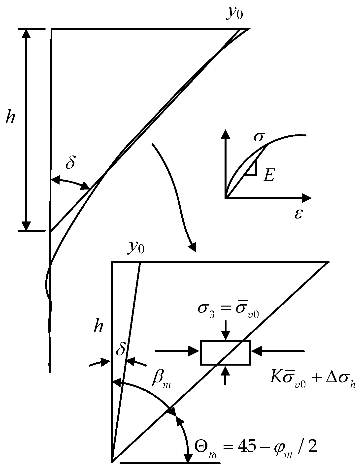
21] iteratively calculates the maximum depth of the wedge based on the global stability and simplifies the lateral displacement of the pile. It is assumed that the displacement of the pile changes linearly within the depth of the wedge, and the deflection angle is defined as
. The linear displacement assumption simplifies the calculation, but it will cause some problems. Xu et al. [
22] believed that at the maximum depth
h of the wedge, due to the assumption of linear displacement, the actual deflection angle was much smaller than the assumed deflection angle
, which makes the calculated subgrade reaction modulus far too large, and singularities appear. To correct this problem, Xu et al. [
22] restricted the upper limit of
k directly.
It is noted that with the increase of the lateral load on the pile top, the shallow rock is first destroyed and gradually develops to the deep layer, and the strain is unevenly distributed throughout the wedge.
For this reason, this article has made the following amendments to the development of pile deformation:
Assuming that the lateral deformation of the pile at the depth of each layer no longer changes linearly along the depth but is independent of each other, the strain wedge in front of the pile is shown in
Figure 5.
Suppose the lateral deformation of the
i-th layer of pile is
yi, the strain of the
i-th layer of soil is
. Moreover, the relationship between the deflection angle
of the
i-th layer of pile and the displacement of the pile is:
Correspondingly, the strain of each layer of soil in the strain wedge is also independent of each other and is related to the lateral displacement of the pile. The strain of the
i-th layer of soil is:
where
is the strain wedge length of the
i-th layer of the rock.
4.2. The Relationship between the Lateral Strain ε and the Deflection Angle of the Pile δi
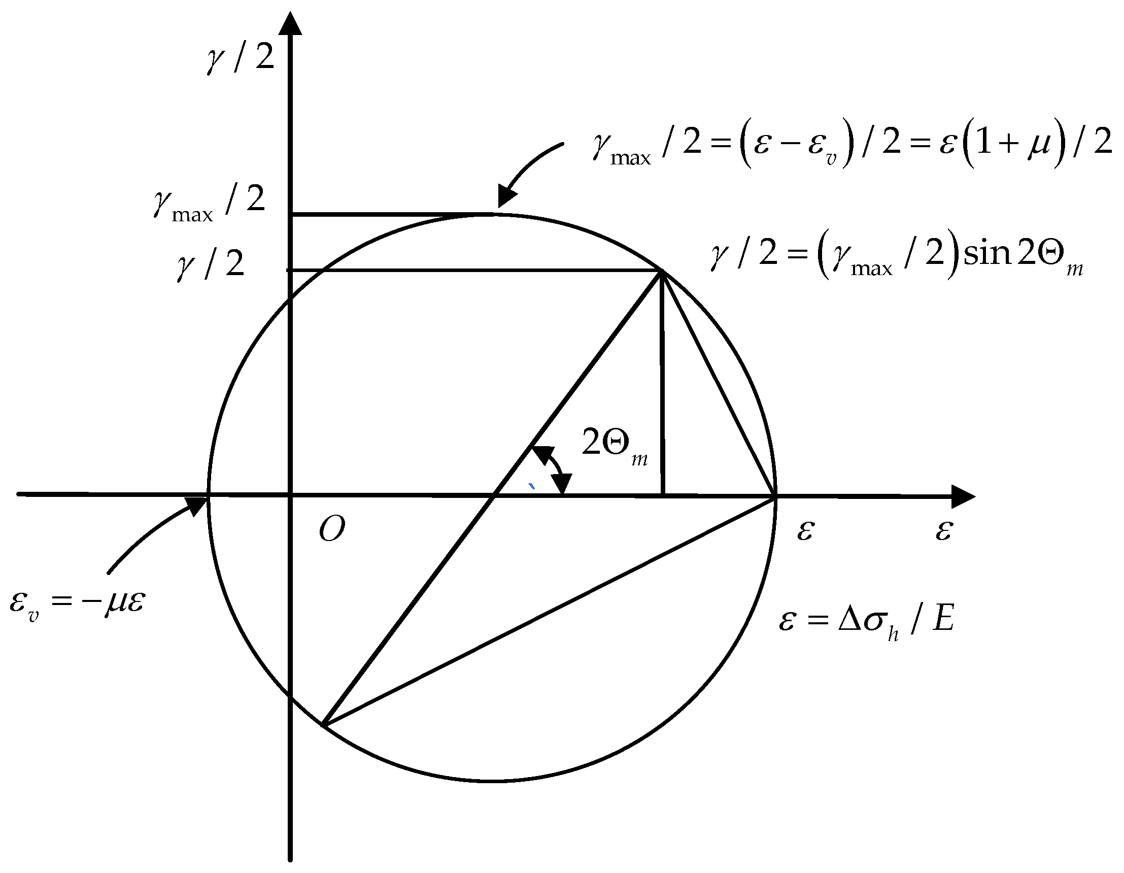
It can be demonstrated from a Mohr’s circle of rock strain, as shown in
Figure 6, that shear strain
, is defined as:
From the relationship between the deflection angle of the pile and the shear strain of the rock, the relationship between the lateral strain of the rock and the mobilized friction angle of the rock can be obtained as:
4.3. Relationship between Lateral Stress Change Δσh and Lateral Strain ε
Ashour et al. [
21] proposed the concept of stress level, combined with the triaxial test of sand and soft clay, and established the relationship between stress–strain and the mobilized friction angle. Ashour used a power function stress–strain relationship, which reflects the nonlinear change of stress level (
SL) with axial strain (
) under constant confining pressure. In order to be suitable for the entire soil strain stage, the form of stage change is used.
However, for intact rock, when the displacement is small, the stress–strain relationship of the rock is mainly linear elastic change. Therefore, the linear elastic model can be used to express the stress–strain relationship:
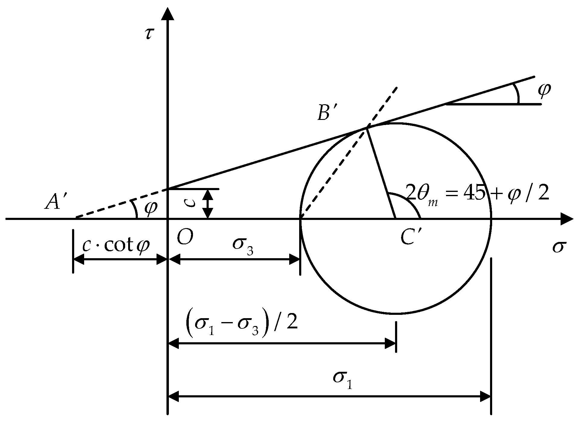
According to the Mohr circle of the limit equilibrium state of rock and soil mass, as shown in
Figure 7:
The relationship between the principal stress can be obtained as:
For sand and soft clay, the cohesion
c is too small to be negligible. Then the maximum principal stress change of soil is:
The relationship between the lateral stress change
and the friction angle of the soil is established through the stress level
SL [
21].
Figure 8 shows the relationship among the lateral stress change, the stress level, and the friction angle.
Stress level in sand:
where the stress change at failure:
Stress level in clay:
where
For rock and soil materials with cohesion–friction properties, the cohesion cannot be ignored, then the Equation (37) becomes:
Therefore, for rock and soil materials with cohesion–friction properties, the stress level calculation method of Equation (38) is no longer applicable. The stress level needs to consider the variation of cohesion with the principal stress. For the convenience of calculation, it is assumed that the cohesion and the friction angle change synergistically, as shown in
Figure 9:
Therefore, the stress level of rock–soil materials with cohesion–friction properties can be expressed as:
Replacing
in the above equation can obtain the following expression:
4.4. Relationship between Pile Side Shear Stress τ and Pile Displacement y
Xu et al. [
23,
24] used the bilinear shear model and the slip-line field theory of the non–gravity obtuse wedge under unilateral pressure to obtain the shear stress of the pile–rock interface during the slip and shear process. Dai et al. [
25] used artificial rocks to simulate soft rock and plexiglass to simulate pile foundations and to study the influence of pile–rock interface roughness on the vertical bearing characteristics of pile foundations. The above studies all believe that the roughness of the pile–rock interface and the rock strength have a significant impact on the vertical bearing capacity of the pile foundation.
However, there are few studies on the relationship among the lateral friction of the pile, the interface roughness, and rock strength under lateral load.
In this study, the hyperbolic method proposed by O’Neil et al. [
26] and Jeong et al. [
27] was used to express the relationship between the lateral friction of the pile–rock interface and the lateral displacement of the pile foundation.
According to Horvath et al. [
28], a method for calculating the maximum lateral friction resistance was proposed based on the full–scale test pile data of 6 soft rock–socketed piles.
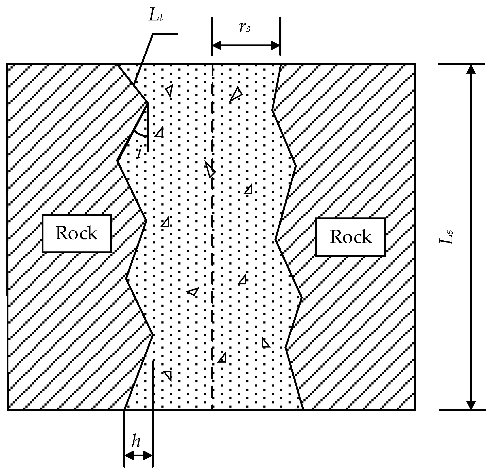
where
is the roughness factor (
Figure 10);
is the average height of asperities;
is nominal socket radius;
is total travel distance along the socket wall profile;
is nominal socket length.
The expression of pile side friction resistance can be obtained. However, only half of the pile foundation is calculated:
4.5. The Relationship between p and (Δσh, τ)
The horizontal stress change (
) is constant across the width of the trapezoid BB’C’C (of face with
of the passive wedge) is shown in
Figure 3. Moreover, the rock resistance per unit pile length is obtained from the balance condition of the force [
21]. The ultimate load per unit length at
x depth is:
where
S1,
S2 is factor of pile type, and
S1 = 0.75,
S2 = 0.5 for circular pile cross section; and
S1 =
S2 = 1.0 for a square pile.
Alternatively, one can write the above equation as follows:
where
A is ratio between the equivalent pile face stress and the lateral stress change.
Referring to the normalized pile deflection shape shown in
Figure 4 and Equation (34):
It can be obtained that the relationship between the linear deflection angle and the lateral deformation of the rock:
Based on the above analysis, the final expression of the subgrade reaction modulus can be obtained:
The maximum depth h of the strain wedge corresponds to the global force balance depth of the pile–rock system.
Equation (28) can be solved by numerical methods by substituting Equation (56) into Equation (28).
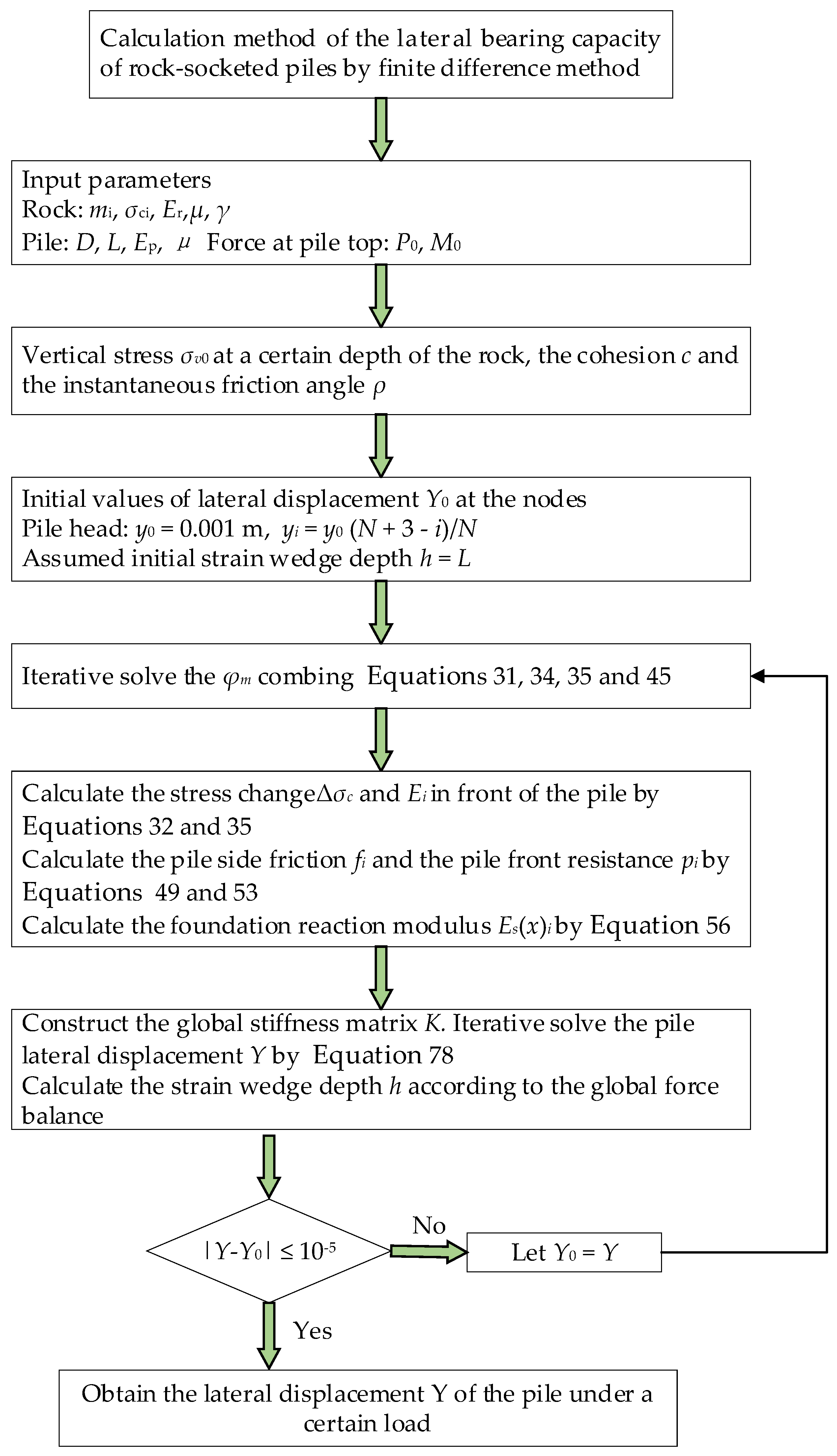
4.6. Strain Wedge Model Solution Method and Flow Chart
Because the obtained subgrade reaction modulus is too complicated to solve by analytical method, the difference method is used to solve Equation (28) in this paper.
Use Taylor series to expand the expression
of pile horizontal displacement function forward and backward:
Combining Equations (57) and (58) can be obtained:
Omit the higher-order infinitesimals to obtain:
In the same way, combing Equations (57)–(60) can be obtained:
Divide the total length L of the pile into N sections, each section having a length of h = L/N. In order to use the finite difference method to solve the problem, two virtual points were added above the pile top and below the pile tip, numbered 1, 2, and (N + 4), (N + 5), respectively. There was a total of (N + 5) nodes along the pile length. The number of pile top is 3, and the number of pile tip was (N + 3).
Substitute Equation (66) into Equation (28)
where
,
,
,
,
correspond to
,
,
,
,
respectively.
The finite difference form of Equation (28) can be obtained:
Equation (68) has (N + 1) equations in total.
For long piles, the pile tip bending moment and shear are zero. From the reference [
19]:
When the pile tip bending moment and shear force are zero, the following condition can be obtained:
Pile head conditions:
When the bending moment
and lateral force
of the pile head are known:
When the bending moment
and rotation angle
of the pile head are known:
There are total (
N + 5) equations include the differential Equation (68) pile tip conditions Equations (72) and (73) and pile head conditions Equations (74) and (75) or (76) and (77):
where
is the coefficient matrix of the equations;
is the lateral displacement vector of the pile including the virtual point;
is the vector formed on the right side of the equations.
It can be solved by iterative method. The solution process is shown in
Figure 11.
5. Approach Verification
Liang et al. [
4] obtained a series of responses of rock socketed pile under lateral load based on field tests. Referring the tests, parameters of rock were used to verify the reliability of the method proposed in this paper by numerical method. Rock and pile foundation parameters adopted in this paper are shown in
Table 1 and
Table 2.
Figure 12 shows the meshes of a single drilled shaft–rock system created using FLAC3D. The bottom and lateral boundary of the rock are fixed. The drilled shaft is modeled as an elastic material, while the rock is modeled using the Hoek–Brown model. The interface between the pile and rock is modeled using the theory of interface.
Figure 13 shows the load–displacement curve of pile top calculated by numerical analysis method and proposed method. Under a certain load level, the horizontal displacement of the pile top and the load are approximately linear.
Figure 13 shows that the method in this paper is in good agreement with the numerical analysis method.
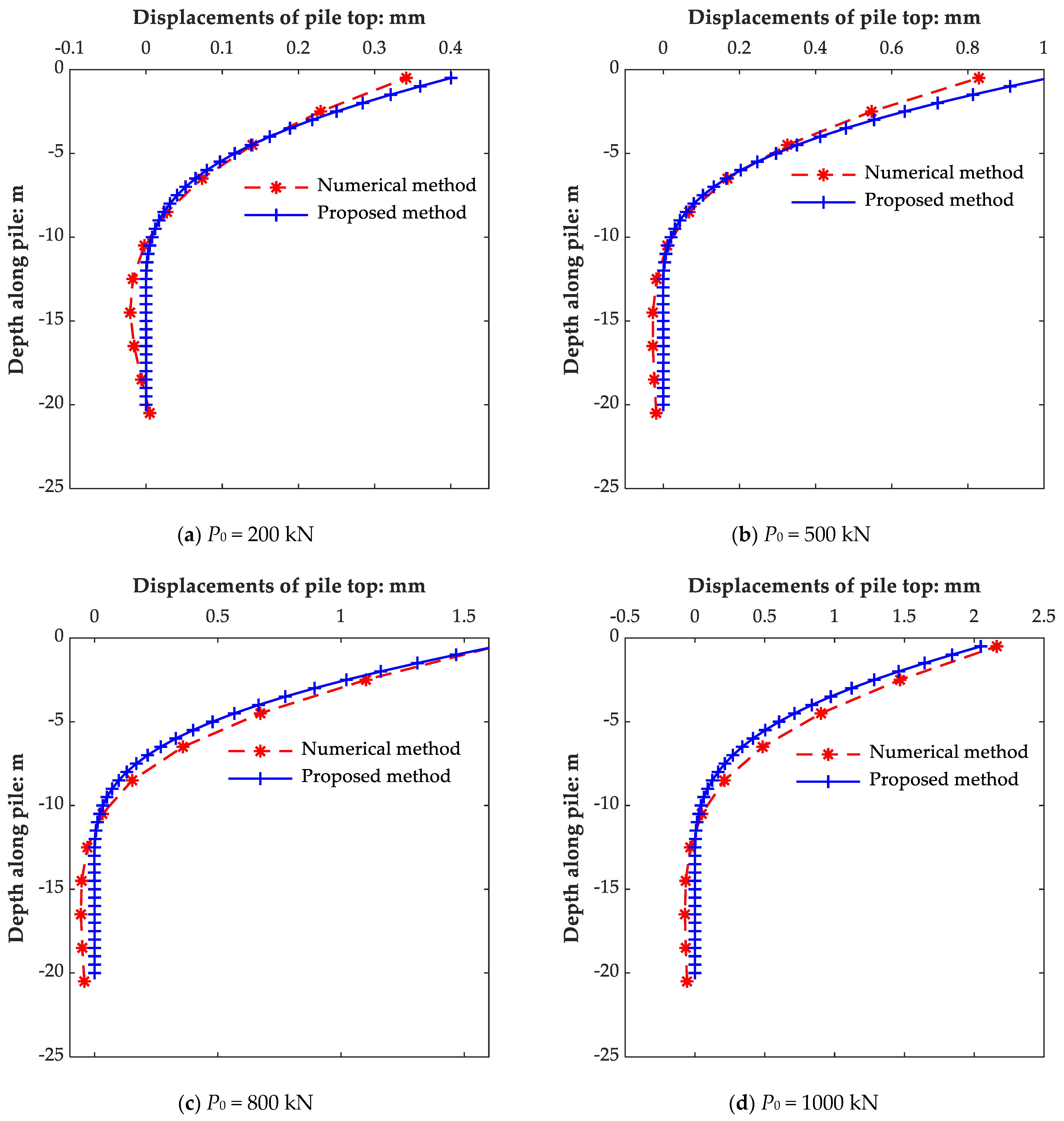
Figure 14 shows the distribution of pile displacement as the lateral load on pile top is 200 kN, 500 kN, 800 KN and 1000 KN, respectively. It can be seen that the proposed method in this paper is in good agreement with the numerical results. Although there is some difference in displacement along the pile, the curves have the same change trend. The variation of pile displacement conforms to the numerical calculation results, which can be used to guide engineering practice. However, the depth of strain wedge is smaller than the numerical results, which needs further correction.
Because the parameters used in this paper are general parameters, this method has further popularization significance. It can be used for engineering design after actual engineering verification.
6. Conclusions
Based on the Hoek–Brown failure criterion used in rock engineering, a p–y criterion for rock is developed in this paper. The concept of the instantaneous angle of friction is employed to deduce the formula of lateral bearing capacity of rock–socketed piles. Based on the strain wedge model, the formula of p–y curve of rock–socketed pile is obtained, and the differential equation is solved iteratively by the finite difference method.
The strain wedge model is modified from three aspects: the assumption of nonlinear displacement, the stress level related to cohesion and friction angle, and the pile side resistance. A numerical method is given to verify the rationality of the modified strain wedge model. The modified strain wedge model can better predict the pile deformation.
However, this paper is based on complete rock calculation, and further research is needed for jointed rock mass.


