1. Introduction
There is a shortage of new construction workers in the industry due to the trend of laborers wanting to avoid extreme environments [
1]. Particularly, due to the retirement of older workers, there is a shortage of skilled workers. Therefore, research is being conducted on autonomous trucks and construction robots that can replace humans at construction sites. Excavators are considered low risk because they do not travel at high speeds, and they perform repetitive tasks. Hence, their automation is highly feasible. For this reason, major construction equipment manufacturers are incorporating various types of automation [
2,
3]. Diverse research was carried out in line with this trend. For example, several publications examined the automated determination of excavation spaces and related control techniques [
4,
5,
6,
7,
8,
9,
10,
11]. An excavator digs up and transports loads into the cargo box of heavy-duty dump trucks. Excavators feature long joints and are often positioned at the rear of a truck to load materials. After the cargo box has been loaded sufficiently, the process is repeated for additional trucks.
To automate this process, it is vital that the excavator acquire accurate information about the cargo box’s three-dimensional (3D) position for analysis. Stentz introduced a method for recognizing a truck’s cargo box after segmenting a truck from dense Lidar data [
12]. The truck’s cargo box is scanned using a dense LIDAR sensor. After segmenting the cargo box from dense rider data, the 3D position of the dump truck is determined by the upper plane of the cargo box. However, suppose the excavator is positioned higher than the truck, and the truck is parked to the excavator’s side. Stereo cameras are efficient sensors that provide dense 3D depth maps. J. R. Borthwick introduced technology for recognizing the location of a truck using depth information obtained from a stereo camera [
13]. The 3D pose is estimated using the 3D shape information of the truck. A truck cargo box is formed from several faces. The 3D position of the truck is calculated by matching all cargo box planes and the plane of the initial 3D model. Therefore, 3D shape information of the entire truck is required. This method can be used for very large excavators, but it is difficult to apply to general excavators with a low height.
Moreover, there is a way to load a load into a truck by using the structure after installing a special structure [
14]. Since the truck is located inside the special structure and the excavator knows the 3D position of the special structure, the truck’s location is naturally estimated. This method allows the excavator to locate the truck’s 3D location reliably, but it is costly and limited in the location of the structure.
Another option is to place the sensor in a third location other than excavators and trucks [
15]. After installing the GNSS sensor that indicates the location of the truck and excavator, the initial 3D location of the truck and excavator is expressed in a global coordinate system. Next, the three-dimensional position of the truck is estimated using four lidar sensors and fish-eye cameras installed on the excavator. This method increases the cost of configuring the sensor.
Despite the wide variety of dump truck types available, their cargo boxes generally resemble hexahedrons. Furthermore, the box’s door is a flat plane shape for simplified fabrication. This paper describes a technique that enables an excavator at the rear of the loading truck to recognize its 3D cargo box and to estimate the 3D position of the loading space and the volume of the load inside using data obtained from a novel sensing device assembled for this purpose.
Specifically, this research provides the following three innovations:
A novel dump truck cargo box sensing device;
A method of automatically estimating the 3D position of the loading space;
A method of automatically estimating the volume of the load.
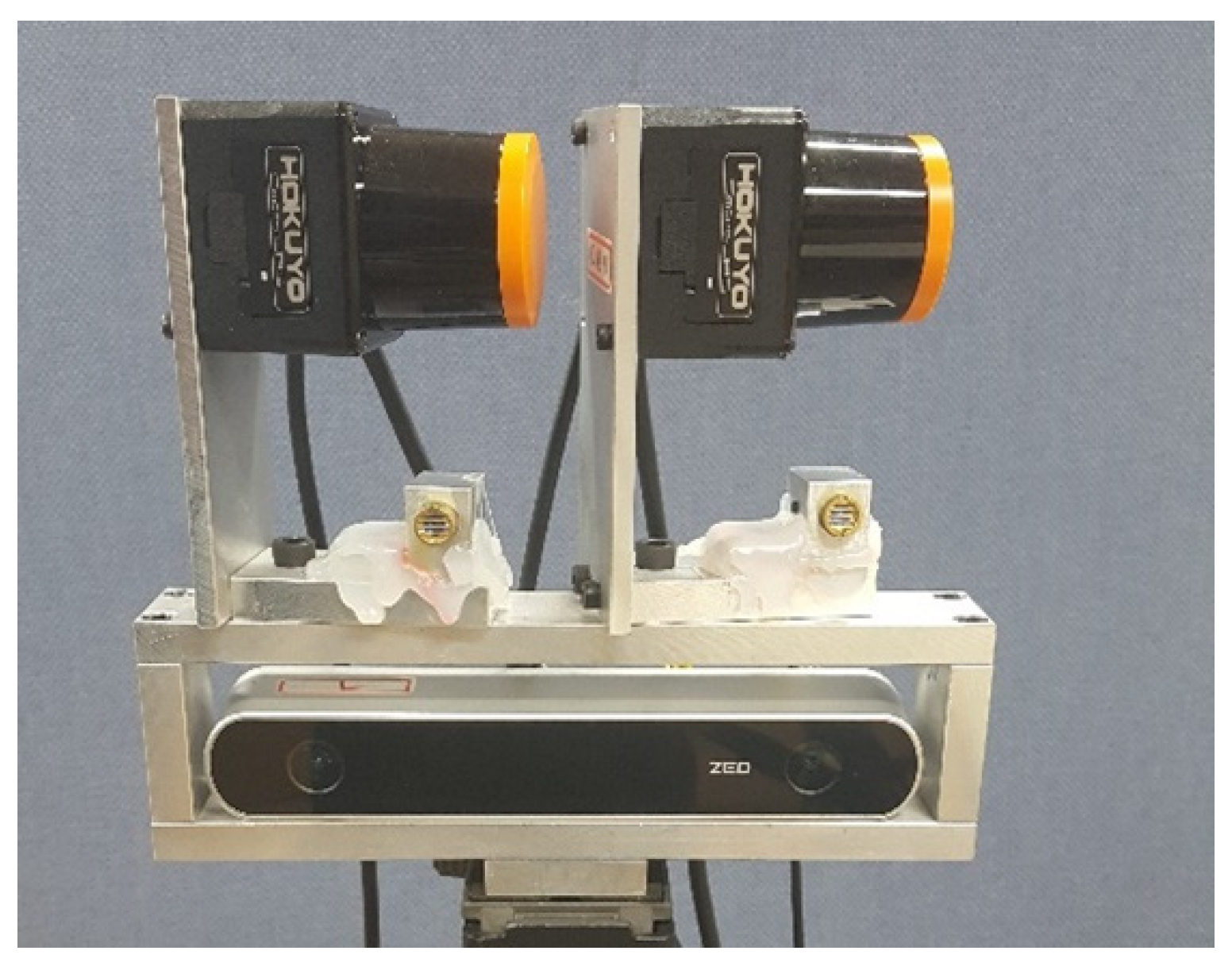
The sensing device combines two two-dimensional (2D) LiDAR sensors and a stereo camera. The scenario includes an excavator operating in an outdoor environment. Note that using only a stereo camera would be hazardous. Hence, two LiDAR sensors complement it (
Section 2). The distance values acquired by each sensor are projected onto one coordinate system using a calibration board and a line laser for accuracy (
Section 3). As the cargo box door resembles a plane shape, the 3D estimation of the position of the cargo box is achieved by determining the plane of the rear of the cargo box from the data received from the two LiDAR sensors installed vertically on the sensing device (
Section 4.1). Furthermore, the 3D position of the box is determined by projecting the dense 3D location of the door acquired from the camera onto a plane and matching it with the actual 3D model of the cargo box. The 3D position of the box can be obtained by utilizing one virtual matching point and four matching points of the rear plane (
Section 4.2).
If the 3D position of the cargo box is estimated solely using the plane, errors may occur. Therefore, points along the long shaft of the box are used for more accurate determination. By matching the sampling of the points of the box’s long shaft to the actual 3D model, the distance data of the shaft obtained from the stereo camera are fed to an iterative closest point (ICP) algorithm (
Section 4.3). Lastly, after the 3D position of the cargo box is estimated, the volume of the load is calculated. Moreover, the 3D position information for the loading space is transmitted to the excavator.
The general outline of this paper is as follows. First,
Section 2 describes the sensing device developed for this study. In
Section 3, the method of calibrating the sensors of the sensing device is discussed.
Section 4 outlines the method for estimating the truck cargo box using information acquired from the sensing device.
Section 5 examines the accuracy of the proposed method for estimating load volume and determining the loading space. The study concludes with
Section 6.
3. Sensor Calibration
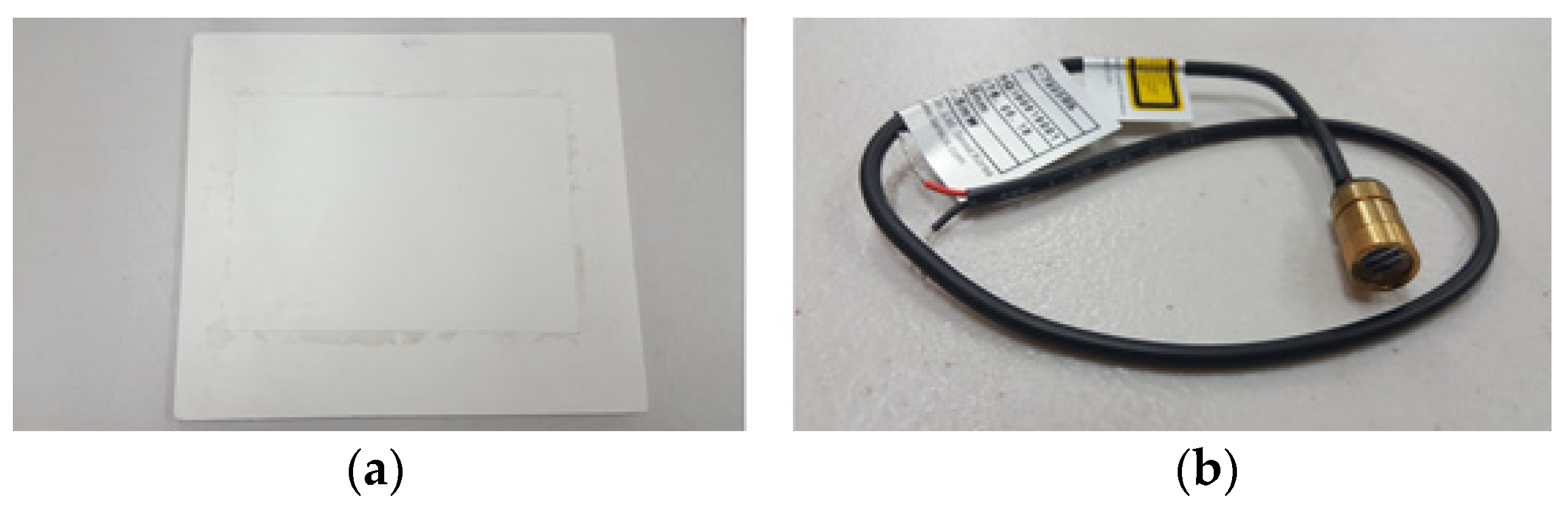
During the scanning process, the depth information from each sensor can be retrieved in real-time. However, the 3D depth information depends on the coordinate system of the sensor. Therefore, it is essential to define a method for representing depth information in a single coordinate system via sensor calibration. For ease of calibration, the line lasers and a flat calibration object were used, as shown in
Figure 2.
Generally, low-cost, mass-produced LiDAR sensors have a bandwidth of 905 nm. The scanning area with the infrared (IR) filter removed captures the laser lines [
16]. Hence, when the line laser and LiDAR scan areas are matched, the area to be scanned by LiDAR can also be determined from the stereo camera image, as shown in
Figure 3.
With
T defined as the Euclidean transformation relation between two coordinate systems, the transformation matrix,
T, is represented by a single (3 × 3) rotation transformation matrix,
R, and a (3 × 1) translation transformation vector,
t. When the 3D matching points obtained from the stereo camera and the LiDAR sensor are expressed as Q
i and P
i, respectively, and three matching points theoretically exist, the transformation matrix, T
(L→C), between the two coordinate systems can be obtained as follows:
If there are more than three matching points, the transformation matrix between the two points in time can be obtained using the singular value decomposition (SVD) or the Levenberg–Marquardt (LM) algorithm to minimize the error [
17], as shown in Equation (2):
In order to facilitate calibration, the LiDAR sensors were positioned so that they sensed the calibration board, and the center point of the line was detected by each LiDAR sensor and camera as a match point, as shown in
Figure 4. The distance information of the calibration board scanned by the LiDAR sensor was segmented as a distance value for detection, and the stereo camera used the images to detect the calibration board. Based on the random sample consensus algorithm (RANSAC), the detected lines were fitted more precisely, and the center point was determined [
18].
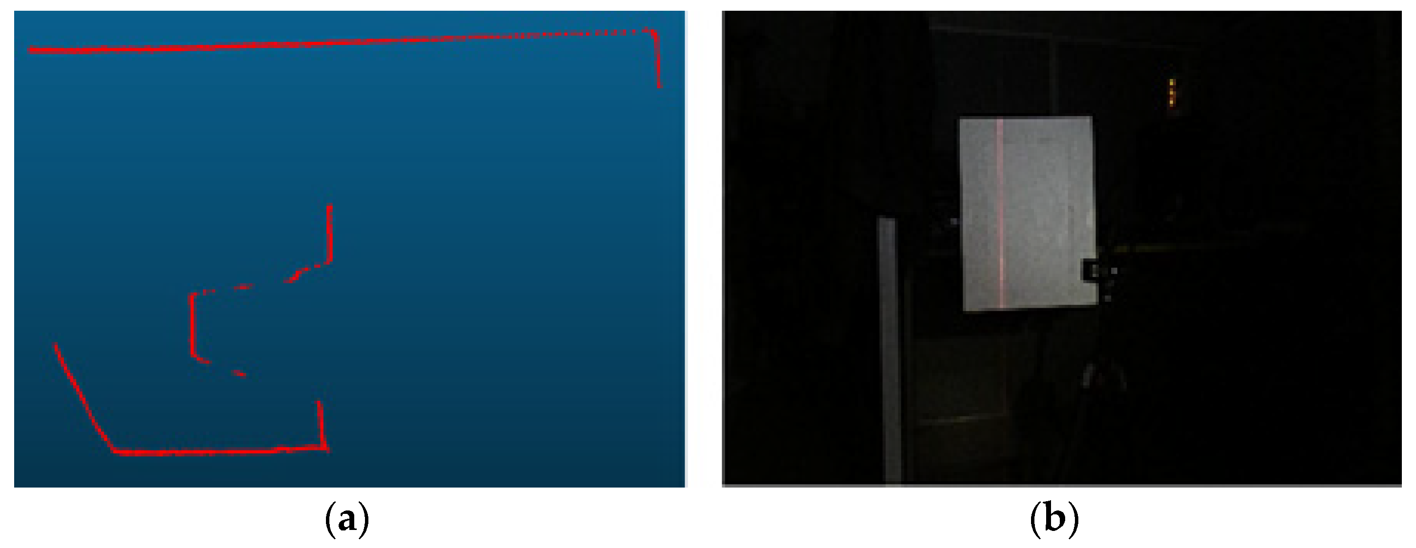
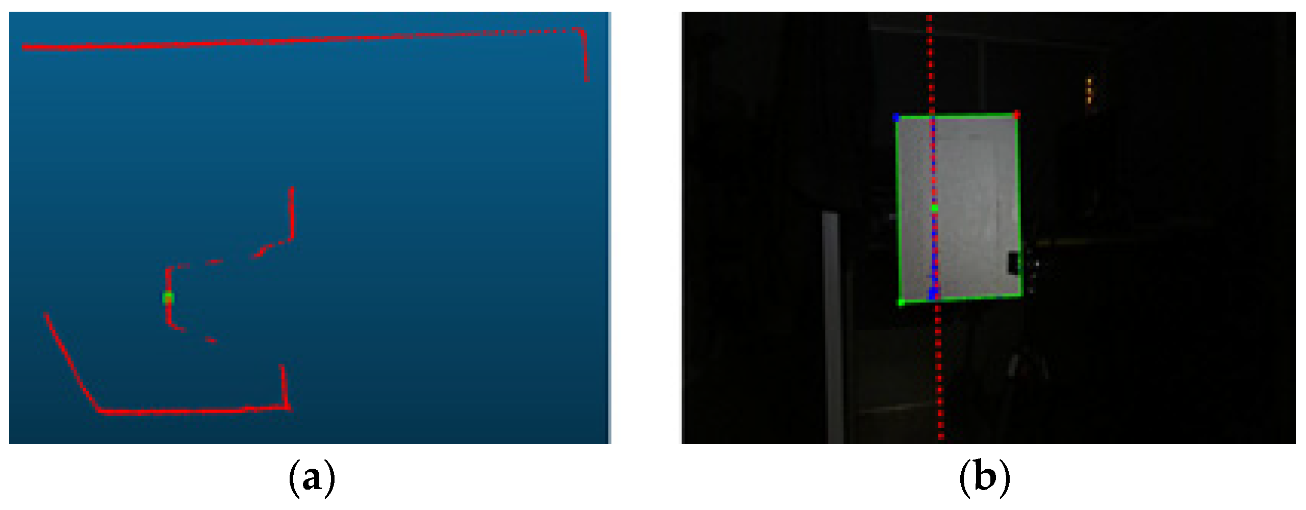
After placing the calibration board at various positions and obtaining the transformation matrices using Equation (2), an accurate projection of the data obtained from the LiDAR sensor onto the position of the line laser was available, as shown in
Figure 5. The accuracy of calibration becomes greater with the increasing number of match points, but this study confirmed that six were sufficient.
Figure 6 shows the results when inter-device calibration was performed and when it was not.
With the calibrated device in the outdoors scan experiment, it is possible to obtain three-dimensional depth information expressed in one coordinate system. In this study, the reference coordinate system of the device was defined as the stereo camera’s coordinate system.
4. Location Estimation of Truck Cargo Box
In order to load the excavator’s content into the truck’s cargo box, it is first necessary to determine its 3D position. Heavy-duty dump truck cargo box doors are flat and generally mounted on the rear of the box. It is characterized by a long shaft emerging from its edge. In this research, the accuracy of the location of the plane was prioritized, assuming the device senses the cargo box door of the truck and that the rear of the cargo box is flat.
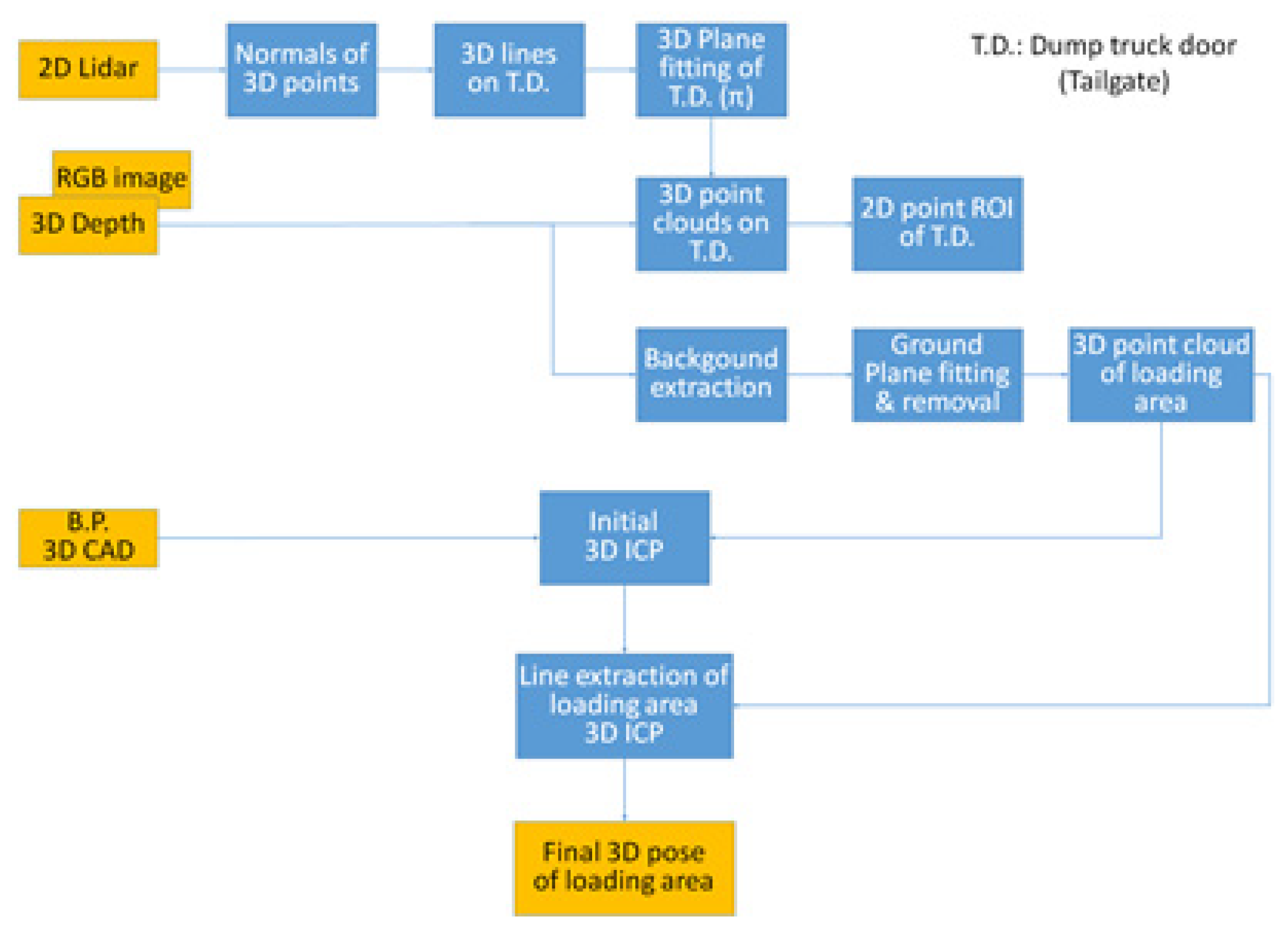
In
Figure 7, a flowchart of the method of estimating the 3D position of the truck cargo box is presented. After the rear of the cargo box is scanned by the device, a dense and sparse 3D point cloud is generated by the stereo camera and the two vertically mounted LIDARs, respectively. Based on the feature points associated with the images on the left and right, the stereo algorithm generates the 3D depth value. Thus, the more distinct feature points detected by the left and right cameras, the more accurate the 3D depth [
19]. Meanwhile, the depth value of a single-color object with few features will have a larger error because of inaccurate matching. It is possible to scatter random patterns to overcome this problem, but they are ineffective in the presence of strong wavelengths of light, such as sunlight [
20,
21].
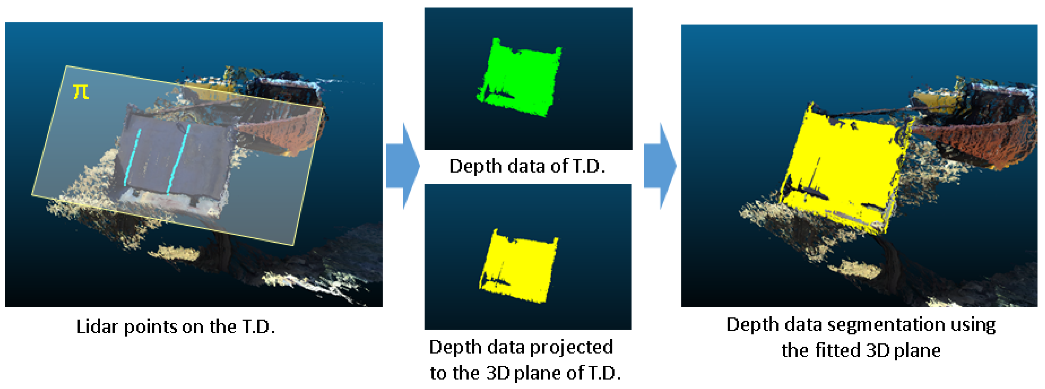
Commercial dump trucks usually have a single-color cargo box, making it difficult for left and right cameras to identify similar features. Consequently, the distance information on the rear side of the dump truck cargo box will be inaccurate. To overcome this issue, two LiDAR sensors that provide constant depth information were used to identify points on the cargo box’s door. The normal vector of the 2D point first obtained from the lidar sensor is calculated using the surrounding points. The points on the door are determined by the distance information between the normal vector and the two LiDAR sensors, and the noise points are removed using a line fitting algorithm. They are then formulated into a plane corresponding to the rear of the cargo box.
A stereo camera provides a dense 3D point cloud. Points close to the plane are points on the door. These points are projected onto a plane and represented as a 2D ROI. Conversely, points that do not exist on the plane are considered noise. These 3D points exist on the ground and are removed using ground plane fitting. As a result, a 3D point cloud of the truck cargo box is obtained.
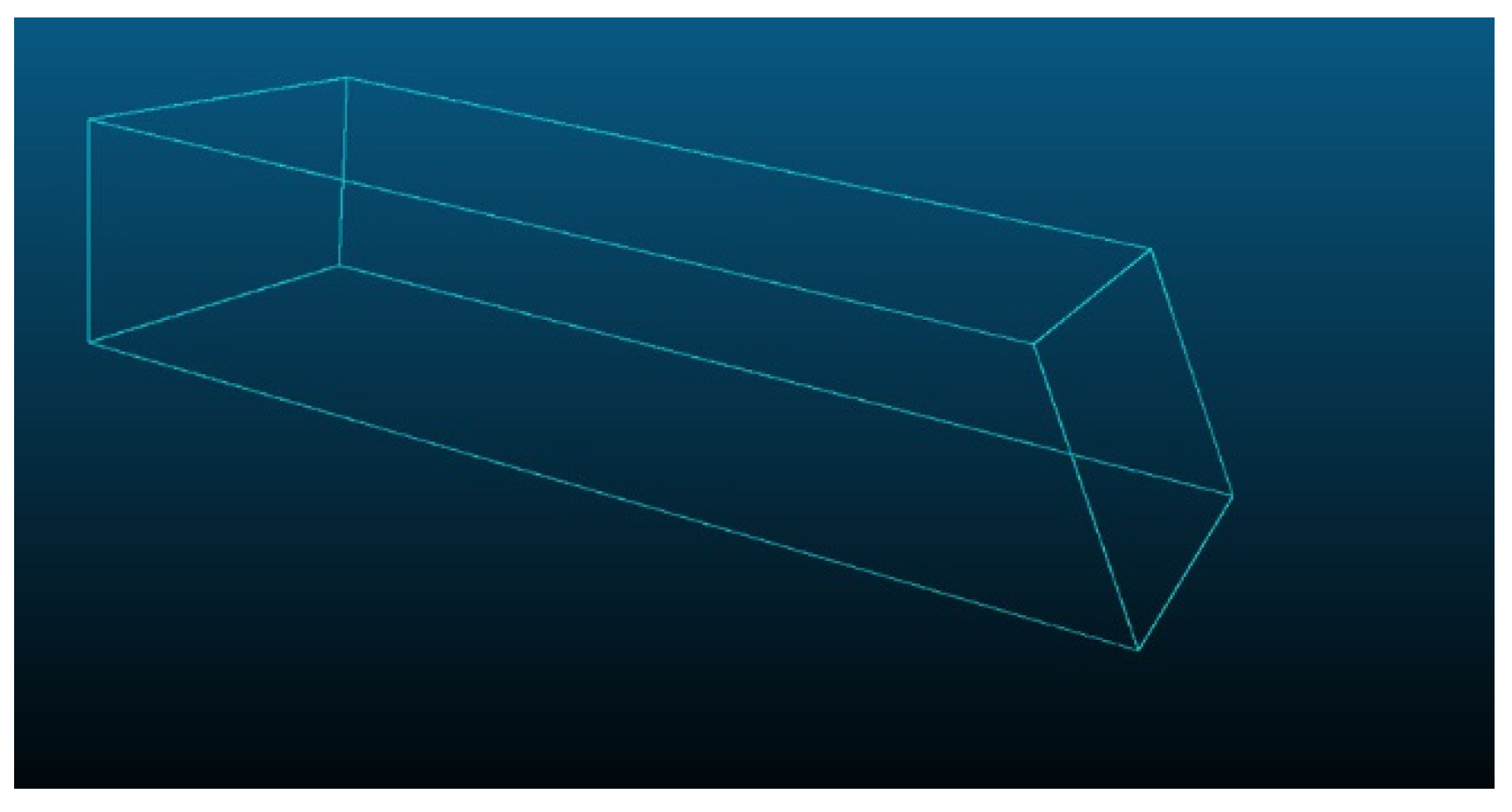
In the next step, we create one 3D hexahedron model with the same dimensions as the cargo box. The initial 3D position of the cargo box is determined by matching the planes of the two models. After estimating the initial 3D position of the box, the estimation error is corrected by using the long axis of the cargo box. A detailed description of each step can be found in the detail section.
4.1. Cargo Box Rear Detection Using a LiDAR Sensor
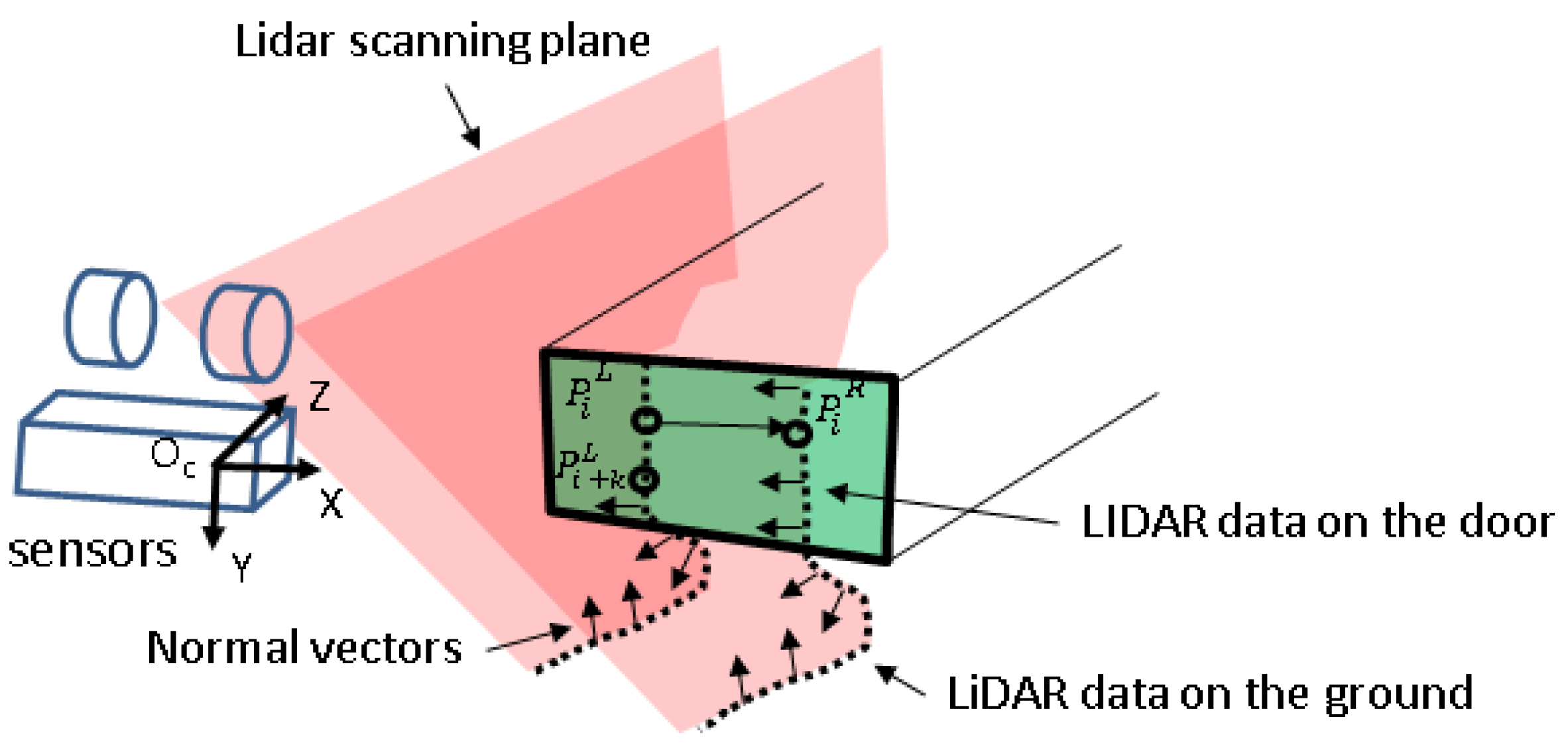
Due to the vertical placement of the two LiDAR sensors, data from the cargo box door and the ground are merged, and the point cloud for the cargo door is separated. In theory, a 3D point cloud on a plane can be described by an identical normal vector. Furthermore, when a sensing device is constructed, the index, , of the point cloud obtained from the two LiDAR sensors may be considered identical if both identical LiDAR sensors are located on the same plane. Therefore, a simple method was used to detect the point cloud on the cargo box door using two LiDAR sensors.
Figure 8 illustrates the process of obtaining the point cloud on the cargo box door. Three-dimensional point clouds acquired from the left and right LiDAR sensors are denoted as
and
And their normal vectors are
and
, respectively. The normal vector,
is determined by the cross product of the two vectors after obtaining the direction vector,
B of
and
(
k is 3–5), after the direction vector,
A of
, is ascertained from,
. The normal vector,
, of the right-side LiDAR data,
, is obtained using the same method. When the normal vector of all point clouds is determined, the dot product and the z-axis (0, 0, 1) of the stereo camera coordinate system are obtained.
As the sensor mounted on the excavator is placed on the rear side of the cargo box, an inner product value closer to −1 is considered to be the point cloud on the cargo box door. The point cloud is filtered using the magnitude of the direction vector, A. Points with significant differences in the distance cannot be considered part of the point cloud and are therefore removed, as they are considered noise. Because the points are discriminated using only the normal vector and the distance between the point clouds, there may be outliers that are not removed from the filtering.
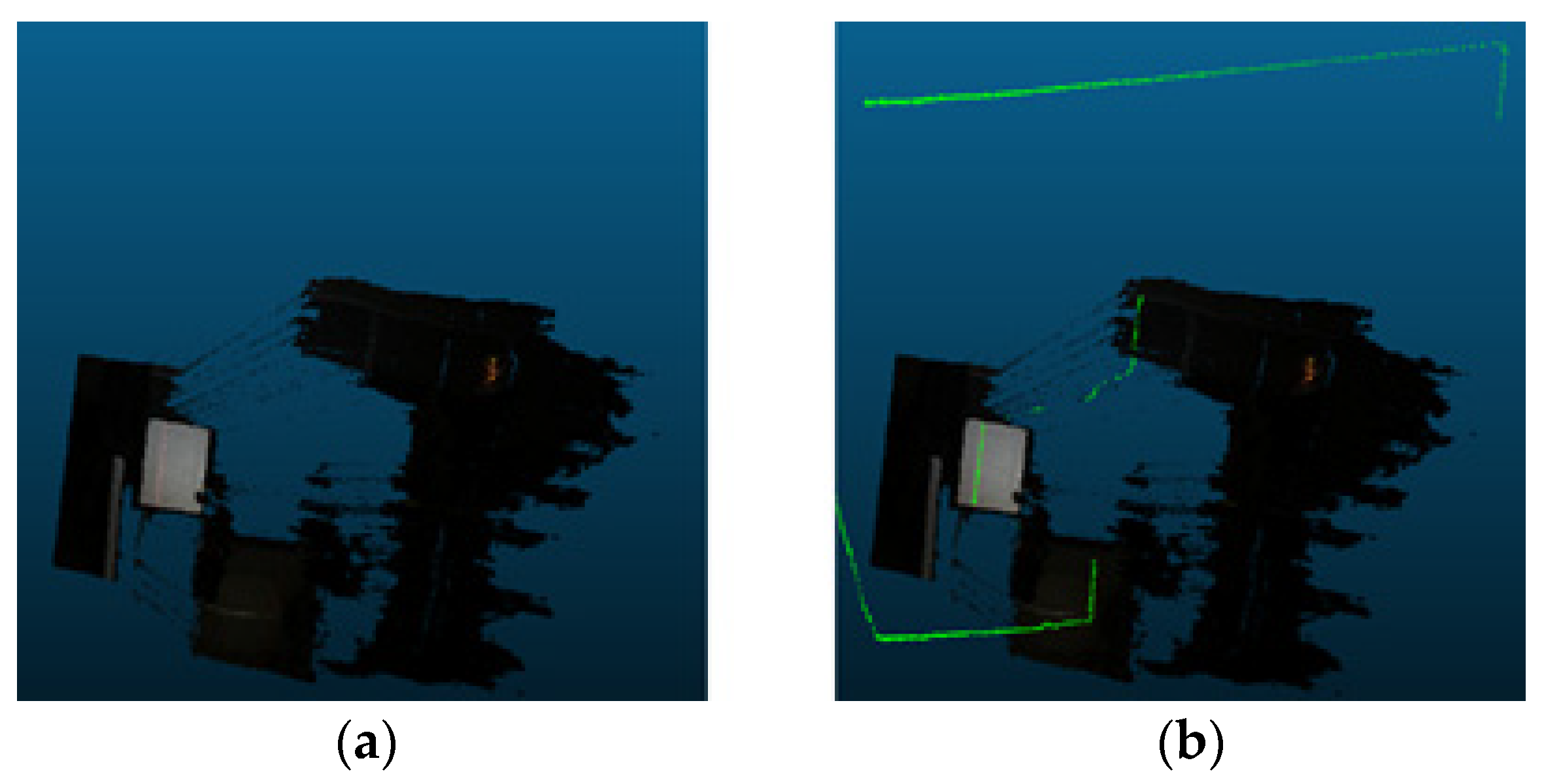
Lastly, outliers are eliminated by line modeling the 3D point cloud sorted using the random sample consensus algorithm, and the final 3D point cloud existing on the cargo box door is sorted.
Figure 9 shows a LiDAR point cloud with outliers removed from a three-dimensional point cloud of a stereo camera. Point clouds that are not line-fitted are considered noise.
This point cloud is used to define the plane of the rear of the cargo box,
, as in Equation (3), and the plane equation is obtained using the least-square method shown in Equation (4):
The matrix form is a linear equation,
. Therefore, the general solution,
, is computed using SVD, as in Equation (5). Finally, the back plate plane is computed with Equation (6):
4.2. Recognition of Initial 3D Position Using a Stereo Camera
Although the box is plane-shaped, the 3D distance provided by the stereo camera does not provide an accurate representation of the shape if the box is single-colored. Consequently, the plane data obtained by the LiDAR sensor on the rear of the cargo box are used to correct the acquired depth value. In the dense depth map obtained from the stereo camera, the 3D point cloud is expressed as
. Hence, the points closer to the cargo box plane must be sorted in advance as they are likely to be situated on the cargo box door. It is possible to calculate the distance between point
and plane
using Equation (7):
Generally, only points with a difference in distance within 30 cm are considered cargo box door points; all other points are regarded as noise and are eliminated. The sorted points can also be projected onto plane
using Equation (8):
Figure 10 shows a projection of the dense 3D point cloud acquired by the stereo camera on the cargo box plane obtained by LiDAR sensors. The distance errors are calibrated as the LiDAR sensor measurement values are projected onto the plane. The projected 3D points can be used to estimate the initial 3D position of the excavator cargo box. The 3D hexahedron model based on the actual dimensions of the box is generated, as shown in
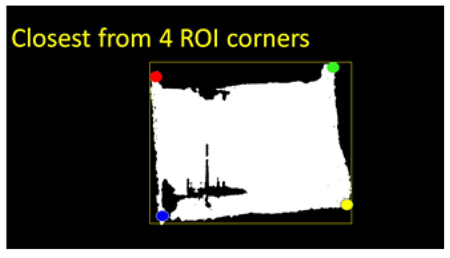
Figure 11. Next, four points near the vertex in the projection points cloud are detected to match the hexahedron model to the actual cargo box plane, as shown in
Figure 12. The points corresponding to the hexahedron model are determined in the same order.
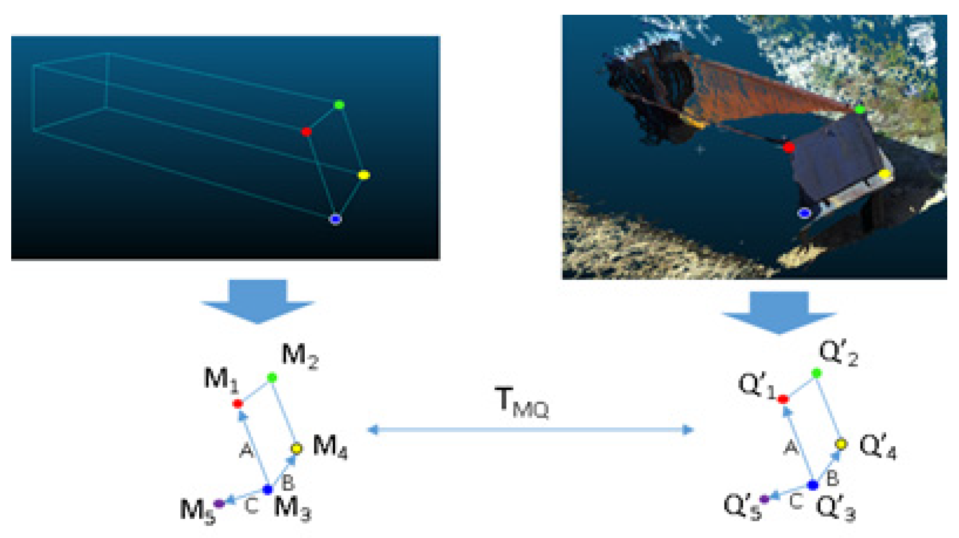
Figure 13 illustrates the method of matching the 3D hexahedron model and the truck cargo box.
First, the four vertices (
,
,
,
) on the 3D hexahedron model and the four vertices (
,
,
,
) on the cargo box plane are set as points of convergence. (
,
) is a virtual point of convergence used to eliminate the symmetry ambiguity. The cargo box has a rectangular parallelepiped form, and its calculation is subject to errors. The virtual point of convergence is determined from the cross-product of each point cloud unit vector,
and
, which become direction vectors of identical magnitude. When the five points of convergence are defined, the 3D transformation matrix,
, is obtained with its error minimized, as in the following equation.
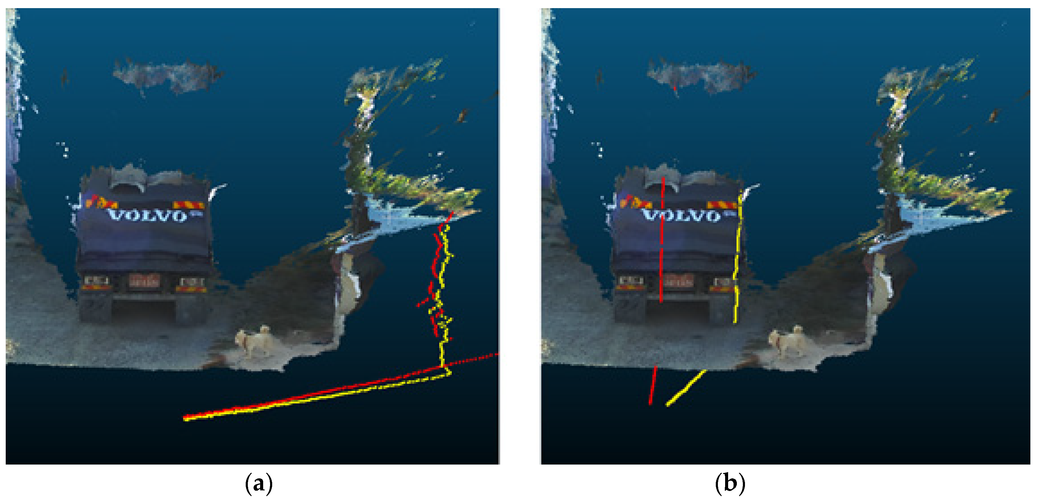
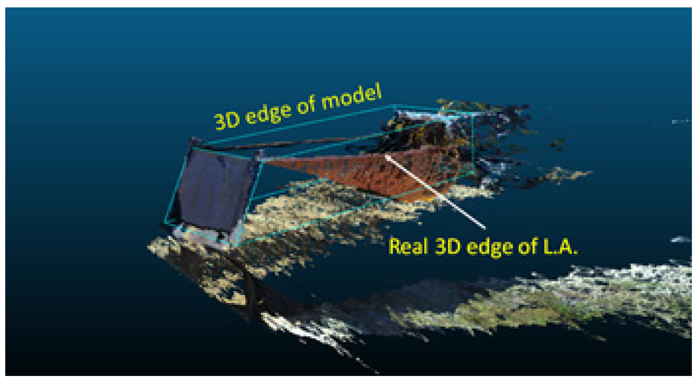
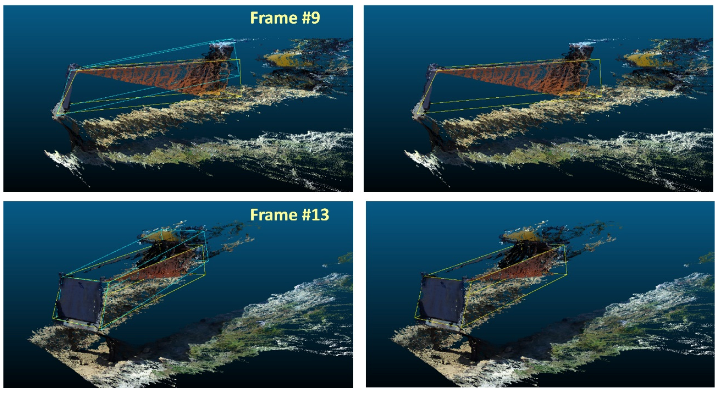
Figure 14 shows the result of matching the cargo box to the hexahedron model using the transformation matrix. The figure shows errors, but a match was made based on the cargo box plane.
4.3. Pose Estimation Refinement
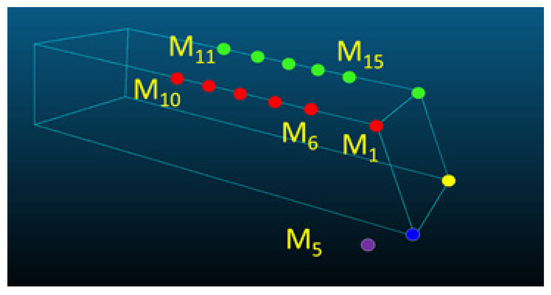
The truck cargo box position was estimated with only five points of convergence results in the errors presented in
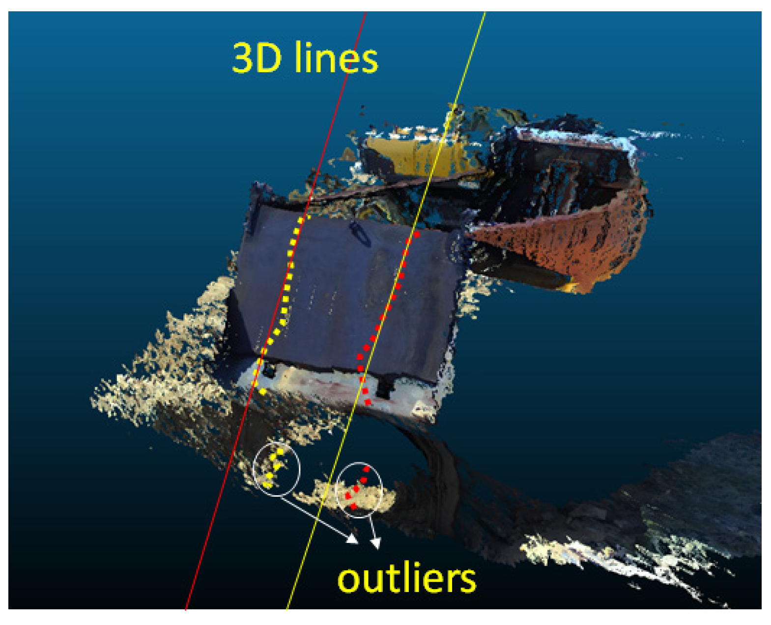
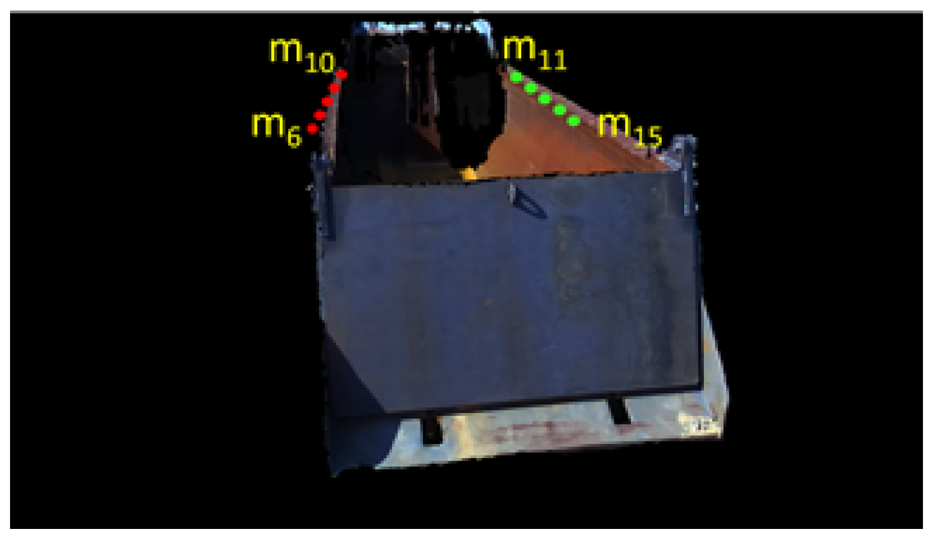
Figure 14. This is caused by differences in the distance information estimated by the stereo camera and the generated 3D hexahedron model. The initial matching results show that more errors occurred at the longitudinal corner than at the rear of the cargo bed. Therefore, to minimize error, the points of convergence are sampled at regular intervals from the two corners along the longitudinal axis of the 3D hexahedron model, as shown in
Figure 15. An iterative algorithm is used so that these points of convergence and the longitudinal axis of the cargo box obtained by the camera will match.
A 3D transformation matrix,
, is used to project the sampled 3D point,
, of the corner onto the camera’s 2D image using Equation (9):
Here,
k is the internal parameter of the stereo camera, and
is the point projected onto the 2D camera image, as shown in
Figure 16. If the initial position transformation matrix,
, is accurate, the projected points are identical to the box corner. Otherwise, they do not match, as shown in
Figure 16. Thus, the longitudinal axis of the cargo box is used to solve this issue.
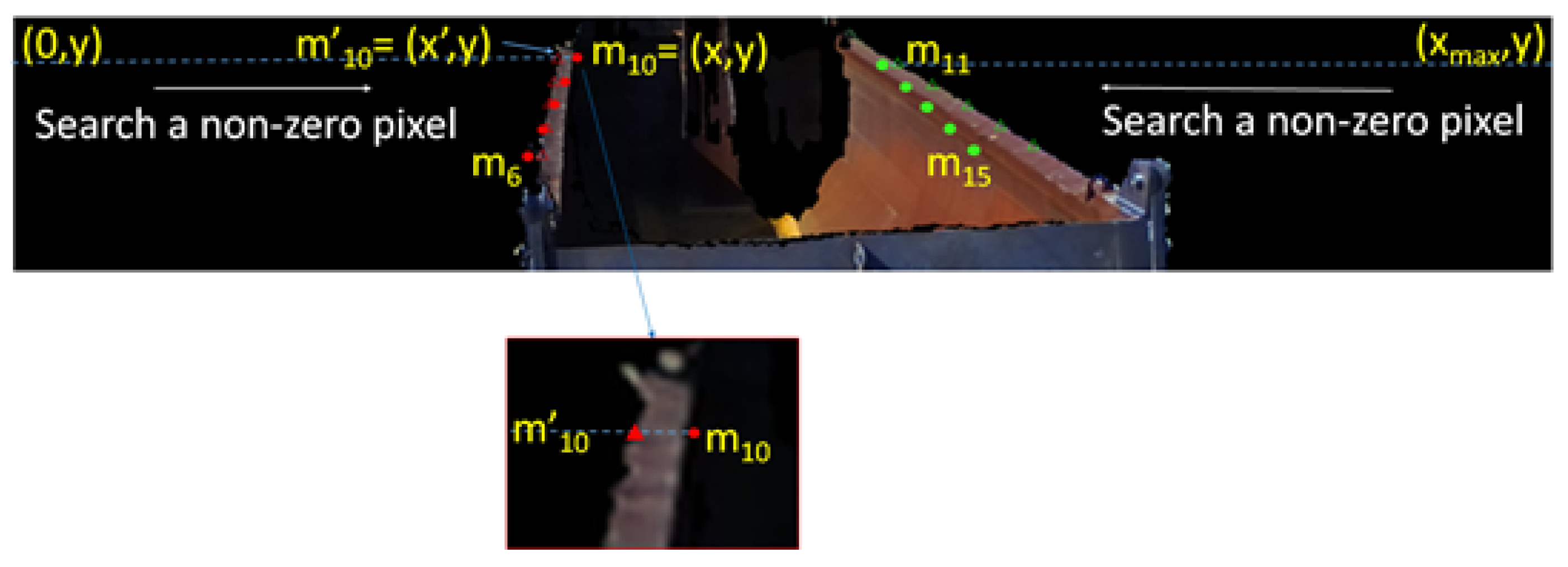
Figure 17 presents the method for detecting points of convergence. When they are projected onto the 2D image, the left corner of the cargo box is searched from the right side of the x-axis, and the right corner is searched from the left side. When a 3D value exists on the searched point, it is designated as the point of convergence. The initial transformation matrix,
, is refined after the ICP algorithm iteratively minimizes the errors of the points added to the corner and the plane [
22,
23]. The pseudocode of the iterative refinement is shown below:
|
| |
| // Find the corresponding points where the distance between |
| |
| |
| // Find the T matrix that minimizes the error. |
| |
| |
| // convert to global coordinate system. |
| |
5. Results and Analysis
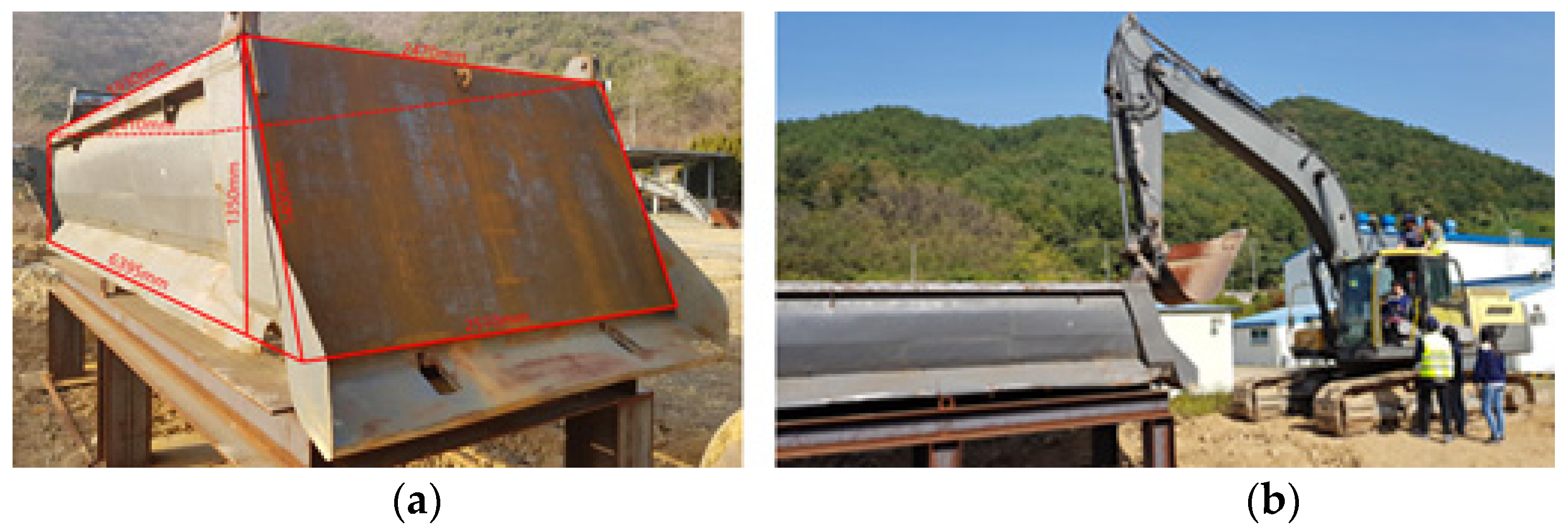
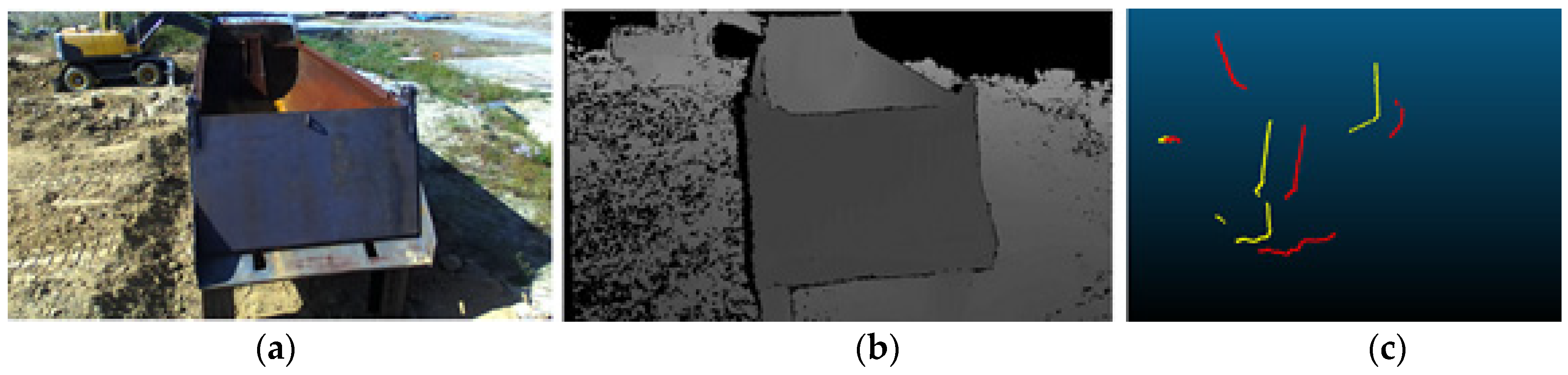
In order to validate the performance of the proposed system, a model of the cargo box of a common heavy-duty dump truck was developed, followed by outdoor experiments. The excavator sensor was installed on the upper section of the driver’s seat of the excavator as shown in
Figure 18, and the loading procedure was repeated 20 times as the sensor sensed the cargo box while the excavator was moving. The data, as shown in
Figure 19, were obtained each time, and the distance values were derived from the stereo sensor.
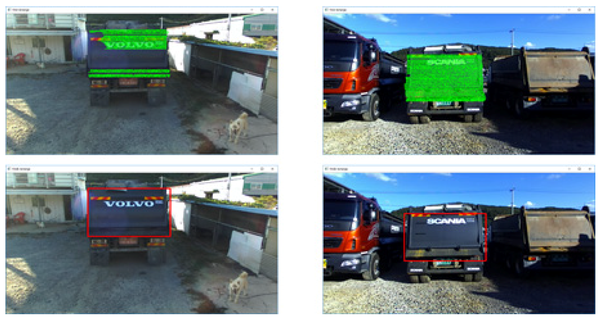
Figure 20 illustrates the detectability of the truck cargo box door based on distance measurements from the LiDAR sensor. When the distance data obtained by the LiDAR sensor and the stereo camera were visualized, only those points that were estimated to represent the cargo box door were visible. Notably, the widely used dump truck cargo boxes of Volvo and Scania were sensed, excluding the experiment model, and an experiment for detecting the cargo box door was conducted [
24,
25]. Using the plane data obtained from the LiDAR sensor, the 3D point cloud obtained from the camera was projected. The cargo box doors of two regular trucks are also detected
Figure 21 shows the experimental results of 3D location estimation using the experimental model. The initial results are indicated in blue, and the more precise results using a refined transformation matrix are expressed in yellow. When the initial position was estimated only using plane data, numerous differences were found in the longitudinal axis of the cargo box. The 3D position estimation using the values obtained by the refined transformation matrix showed that the longitudinal axes of the cargo box and the hexahedral model were similar, indicating that the 3D location estimation was successful. Estimation of cargo space volume can increase work efficiency [
26,
27]. The 3D location of the estimated cargo box enabled the provision of data of the loading space of the cargo box.
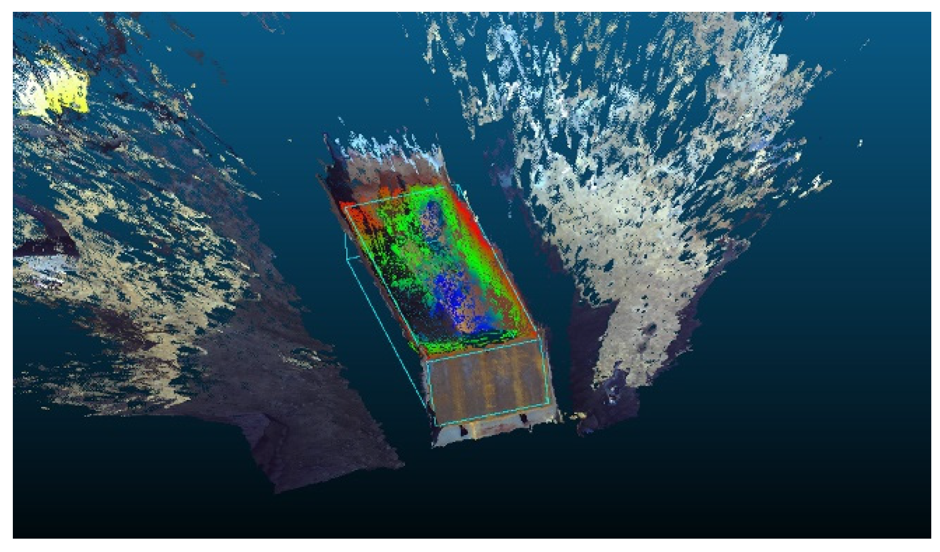
Figure 22 illustrates the visualized results of normalized data based on box height. The load can be placed in the cargo box, excluding the part in red.
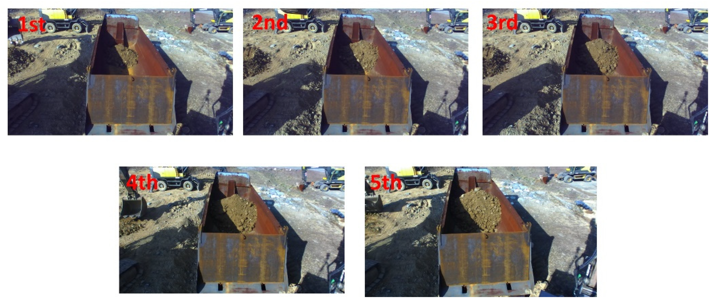
In this study, the load was loaded five times to the cargo box interior using the excavator, as shown in
Figure 23, and volume estimations were made using the image data obtained from the camera. The cargo box interior was detected using the image data when the 3D hexahedral model was projected onto the image, as shown in
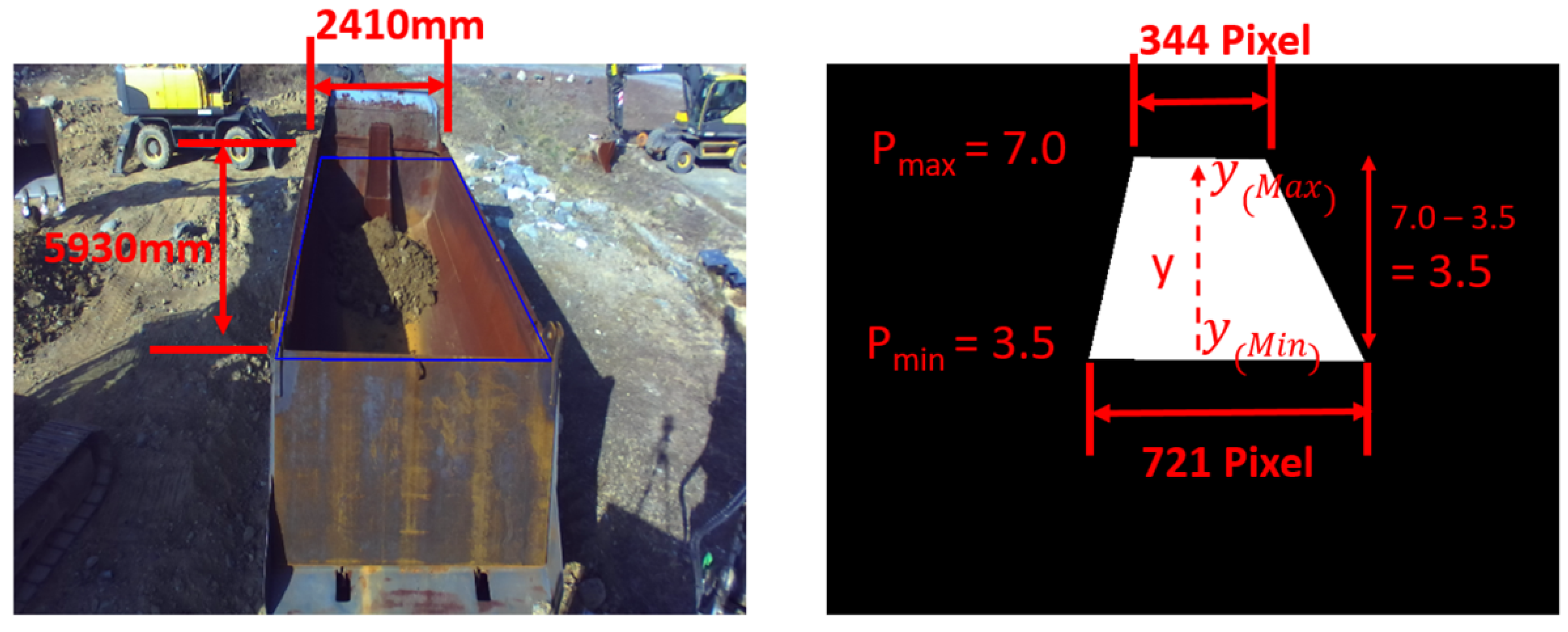
Figure 24. As such, the outcome of the projected 3D points was expressed in the shape of a trapezoid (near–far effect), for which the distance per pixel was considered to estimate an accurate value. The distance per pixel,
, is calculated using Equation (10):
The internal volume of cargo box A obtained from the 2D image is determined using Equations (11)–(13):
Here, is the height value from the model’s floor. The volume of the load was measured using the data from five sets of experiments. The quantitative values were estimated for each loading operation using the difference in volume between frames. The volume of the excavator’s bucket was 0.8 m3; hence, load volume was estimated with the difference in volume estimated from one experiment among the accumulated volume of the load over five sets of experiments.
Table 2 summarizes the measurement results of load volume. Accuracy was determined by the proximity of the value to the ground truth, and the experiment results showed large errors.
The sensing device mounted on the excavator was positioned diagonally rather than accommodating a top view. However, as the cargo box is filled with load, more accurate results are possible if the loads are closer to the sensing device and a more precise camera is used.


