Counterfactual-Based Action Evaluation Algorithm in Multi-Agent Reinforcement Learning

Featured Application

This work can be applied in multi-agent tasks to achieve cooperation between agents. For example multi-agent games, robotic mining, UAV cooperation, social behavior simulation, etc.

Abstract

Multi-agent reinforcement learning (MARL) algorithms have made great achievements in various scenarios, but there are still many problems in solving sequential social dilemmas (SSDs). In SSDs, the agent’s actions not only change the instantaneous state of the environment but also affect the latent state which will, in turn, affect all agents. However, most of the current reinforcement learning algorithms focus on analyzing the value of instantaneous environment state while ignoring the study of the latent state, which is very important for establishing cooperation. Therefore, we propose a novel counterfactual reasoning-based multi-agent reinforcement learning algorithm to evaluate the continuous contribution of agent actions on the latent state. We compute that using simulation reasoning and building an action evaluation network. Then through counterfactual reasoning, we can get a single agent’s influence on the environment. Using this continuous contribution as an intrinsic reward enables the agent to consider the collective, thereby promoting cooperation. We conduct experiments in the SSDs environment, and the results show that the collective reward is increased by at least $25\%$ which demonstrates the excellent performance of our proposed algorithm compared to the state-of-the-art algorithms.

1. Introduction

Reinforcement learning is able to solve the serialized decision-making problem when the agent interacts with the environment [1]. The single-agent reinforcement learning algorithm shows good performance in many scenarios like video games [2], robot control [3], autonomous driving [4,5], etc. However, single-agent reinforcement learning is insufficient to deal with the complex realistic environment containing multiple agents. In multi-agent systems, the agents not only interact with the environment but also need to consider the game relationship with other agents [6]. The involvement of cooperation and competition makes reinforcement learning more complex and interesting [7,8]. Therefore, more researchers have begun to pay attention to the application of reinforcement learning in multi-agent systems.

Early multi-agent reinforcement learning (MARL) was just an extension of single-agent algorithms in multi-agent systems [9,10,11]. According to the different reward function settings, the MARL can divide into two categories. First, in a multi-agent system, all agents are considered as a collective to interact with the environment and get only one total reward [12]. All agents use this reward to update their policies. Thereby, the policy can directly obtain the optimal joint action according to the environment state. However in the face of the dimensional explosion of state space and action space, the policy is difficult to converge and hard to address the credit assignment problem [13]. Another method is that each agent has its own reward function and updates its policy independently [14]. This solves the problems of slow convergence and exploding input space in joint learning. However, ignoring the actions of other agents will lead to the separation between the individual and the collective. Simply applying the single-agent algorithm will make each agent adopt a greedy strategy, resulting in the inability to establish effective cooperation. In conclusion, joint learning and independent learning have their own advantages and disadvantages. However, more scenarios [15,16] require agents to be responsible for different tasks to achieve collaboration, which requires them to learn and make decisions independently.

In independent learning, each agent has its own reward function, and the sum of the rewards of all agents constitutes the collective reward. At this point, for each agent, its contribution to the collective is its own reward. However, some scenarios like Cleanup in SSDs [17] need to be more considerate. In Cleanup, the agent can obtain a reward by collecting apples, and it can also increase the probability of apple generation by clearing the river (however, this action will reduce the agent’s reward). For the latter, we believe that the action, although not immediately rewarding, still contributes to the collective. Therefore, the contribution made by the agent to the environment can be divided into instantaneous contribution and continuous contribution. The former is reflected in the instantaneous reward, and the latter is reflected in the subsequent state. This paper will examine how to assess the often overlooked continuous contribution which is important for establishing agent cooperation. We propose to use the latent state with historical information to evaluate it.

The latent state with more environmental information can be extracted from multiple consecutive observations [18]. Using such a latent state can realize different needs, such as realizing a single agent’s multi-step prediction [19], solving the uncertainty problem in reinforcement learning [20], realizing the prediction of the following environmental state [21], etc. All of these demonstrate that the latent states can be used in solving serialization decision problems in reinforcement learning.

In a multi-agent system, the problem related to determining the contribution of agents is credit assignment [22]. This problem mainly occurs in the centralized reward function setting to determine the contribution of each agent to the team. A common solution is counterfactual reasoning. COMA [23] proposes to train a centralized critic network using a counterfactual baseline. The core idea is “what would happen if I did another action”. However, in COMA, all agents share a reward function, which is not the same as the setting in SSDs. We would prefer to conduct research using a more realistic independent setting.

However, independent learning will also bring many problems. In a multi-agent system, agents attempt to improve their policies based on other agents, whose policies also change over time during training. Such simultaneous changing makes the environment non-stationary [24]. When the agent uses a simple reward function to face a complex environment, most actions do not bring reward. This useful reward for policy updates is sparse across all data [25]. Another very important problem is the competition between agents caused by greedy policies. In order to solve these problems, researchers proposed to divide the original reward into extrinsic reward and intrinsic reward [26]. The extrinsic reward is used to measure agent performance and usually cannot be changed. The intrinsic reward is internal to the agent and is designed to store human knowledge. We use the continuous contribution as the intrinsic reward, allowing the agent to maximize its own reward while considering a greater contribution to the collective.

In this paper, we propose a novel counterfactual reasoning-based multi-agent reinforcement learning algorithm to evaluate the continuous contribution of agent actions to the latent state. A simple approach is simulation reasoning (SR). Using counterfactual reasoning, we replicate the environment at a certain step in the task. We replace the agent’s action with default action in the simulated environment and keep other agents’ policies unchanged. Then we run the simulation environment for K steps and record the data. Comparing the result between real and simulation environment, the continuous contribution of the agent on the environment can be obtained. The second approach is to build a centralized action evaluation network (AEN) to get the continuous contribution. According to counterfactual reasoning, the action of an agent is replaced by the default action and is re-evaluated. The difference between the two is the continuous contribution of the agent to the environment. We take the obtained continuous contribution as an intrinsic reward, and combine it with the extrinsic reward to obtain a reward function that takes into account both the instantaneous contribution and the continuous contribution. By learning through such a reward function, the agent can contribute to the collective while maximizing its own reward.

The main contributions of this article are as follows: First, we discuss the limitations of the current MARL and propose a new counterfactual-based multi-agent reinforcement learning algorithm to obtain the continuous contribution of agent actions on the latent state of the environment. Second, we use the simulation reasoning approach to achieve counterfactual reasoning by replicating the environment and substituting actions. Further, we build a centralized action evaluation network to get the impact of joint actions on the latent states. Finally, we set up experiments on sequential social dilemmas (SSDs) to verify the performance advantages of our proposed methods over the state-of-the-art algorithms.

The rest of this paper is structured as follows: Section 2 describes the basic knowledge of multi-agent reinforcement learning. Section 3 elaborates on the counterfactual-based multi-agent reinforcement learning algorithm with simulation reasoning and action evaluation network. Section 4 introduces the environment and compares the experimental results. Section 5 summarizes and looks forward to the future.

2. Background

We use the Markov decision process (MDP) [27] to represent the process of serialized interaction between the agent and the environment in reinforcement learning. In a multi-agent system, MDP can be represented by a five-tuple M = (S, A, R, T, γ), where S is the state space, A is the action space, $R:S\times A\times S\to \mathbb{R}$ is reward function, $T:S\times A\times S\to [0,1]$ is state transition function, and $\gamma \in [0,1]$ is the discount factor. Agent choose action according to its policy ${\pi }_{\theta }:S\to A$, and receives a reward r. Afterward, the environment will transfer to the next state by T. In a partially observable multi-agent environment [28], $O=O_1\times ...\times O_N$ represent the joint local observation for N agents. $A=A_1\times ...\times A_N$ represent the joint action. Meanwhile, the reward function and transition function change to $R=R_1\times ...\times R_N$, $T=O\times A\times S\to [0,1]$. The discount reward is $R_t={\sum }_{l=0}^{\infty }{\gamma }^l{r}_{t+l}$. Our goal is to find a policy that maximizes the expected collective reward $R_{\theta }=E_{\tau \sim p_{\theta }\left(\tau \right)}\left[R\left(\tau \right)\right]$.

Classical reinforcement learning methods are divided into two categories, one is based on Q-learning [29], and the other is based on policy gradient [30]. Q-learning calculates the value of state-action pair called Q-value:

$$Q_{\pi }(s,a)=E_{r,s^{\prime }}\left(R\right|s_t=s,a_t=a)$$

(1)

Based on the Bellman equation $Q_{\pi }(s,a)=E_{\pi }[r+\gamma Q(s^{\prime },a^{\prime })]$ the Q-value can update by

$$Q(s,a)\leftarrow Q(s,a)+\alpha [(r+\gamma ma{x}_{a^{\prime }}Q(s^{\prime },a^{\prime }))-Q(s,a)]$$

(2)

Silver proposed the DQN [31] based on Q-learning, which uses a neural network to fetch Q-function. The loss function is

$$\mathcal{L}\left({\theta }_i\right)=E_{s,a,r,s^{\prime }}\left[{(r+\gamma ma{x}_{a^{\prime }}Q(s^{\prime },a^{\prime };{\theta }_i^{-})-Q(s,a;{\theta }_i))}^2\right]$$

(3)

The policy gradient algorithm use a neural network to fit policy directly. The gradient is computed by

$${\nabla }_{\varphi }J\left({\pi }_{\varphi }\right)=E[{\nabla }_{\varphi }log\pi \left(a\right|s)Q^{\pi }(s,a)]$$

(4)

The proximal policy optimization (PPO) [32] algorithm uses clip function to limit the magnitude of the gradient update while ensuring the effective update of the policy, and uses experience replay buffer to increase data utilization efficiency. The gradient is computed by:

$$J^{{\theta }^k}\left(\theta \right)=\sum _{s_t,a_t}min(\frac{p_{\theta }\left(a_t\right|s_t)}{p_{{\theta }^k}\left(a_t\right|s_t)}{A}^{{\theta }^k}(s_t,a_t),clip(\frac{p_{\theta }\left(a_t\right|s_t)}{p_{{\theta }^k}\left(a_t\right|s_t)},1-\epsilon ,1+\epsilon )A^{{\theta }^k}(s_t,a_t))$$

(5)

$$clip(a,a\_min,a\_max)=\left\{\begin{array}{cc}a\_min\hfill & \mathrm{if} a<=a\_min\hfill \\ a\_max\hfill & \mathrm{if} a>=a\_max\hfill \\ a\hfill & \mathrm{otherwise}\hfill \end{array}\right.$$

(6)

The above algorithms are classic single-agent reinforcement learning algorithms. In a multi-agent system, a simpler algorithm is to assign each agent an A3C [33] or Q-learning algorithm, like IAC and IQL. However in this way, each agent regards other agents as part of the environment, and does not consider the behavior of other agents when updating, which leads to instability. Therefore, Ref. [34] proposed the MADDPG algorithm and established a centralized critic network to calculate the joint Q value and then update the policy. The gradient formula is:

$${\nabla }_{{\theta }_i}J\left({\mu }_i\right)={\mathbb{E}}_{x,a\sim \mathcal{D}}\left[{\nabla }_{{\theta }_i}{\mu }_i\left(a_i\right|o_i){\nabla }_{a_i}{Q}_i^{\mu }(x,a_1,...,a_N){|}_{a_i={\mu }_i\left(o_i\right)}\right]$$

(7)

The centralized action-value function $Q_i^{\mu }$ is update as:

$$\mathcal{L}\left({\theta }_i\right)={\mathbb{E}}_{x,a,r,x\prime }\left[{(Q_i^{\mu }(x,a_1,...,a_N)-y)}^2\right],y=r_i+\gamma Q_i^{\mu }(x\prime ,a{\prime }_1,...,a{\prime }_N){|}_{a{\prime }_j=\mu {\prime }_j\left(o_j\right)}$$

(8)

Intrinsic reward improves the performance of the RL algorithm and solves the problem of sparse reward [35]. Its general expression is $R=\alpha r_e+\beta r_c$. The former is called extrinsic reward, which represents feedback from the environment. The latter is called intrinsic reward, which contains prior human knowledge that enables the agent to learn faster. Ref. [35] propose to use the influence between agents as an intrinsic reward:

$$r_{c,t}^k=\sum _{j=0,j\ne k}^N[D_{KL}p\left(a_t^j\right|a_t^k,s_t^j)\left|\right|p\left(a_t^j\right|s_t^j)]]$$

(9)

Counterfactual reasoning can be used in multi-agent systems to perform causal reasoning on certain characteristics. At each step, the agent takes turns to simulate counterfactual actions to compare with the real situation. In this way, the agent’s response to the environment or the agent’s response to other agents can be obtained. Counterfactuals can also be used in reward reshaping to solve the problem of credit assignment.

3. Method

In this section, we will introduce the counterfactual reasoning-based multi-agent reinforcement learning algorithm in detail. First, instead of explicitly extracting the latent state of the environment, we compute the continuous contribution by duplicating the environment based on simulation reasoning (SR). Second, we extract latent states from successive environmental states and build an action evaluation network (AEN) to evaluate the continuous contribution of joint actions on the latent state. After getting the continuous contribution, we use it as an intrinsic reward to participate in the update of the policy. The following is the detailed introduction of SR and AEN.

3.1. Simulation Reasoning

In reinforcement learning, the agent updates its policy according to the reward signal feedback from the environment. In MARL, in order to make agents consider the impact of actions on the collective, we give each agent additional intrinsic rewards. Moreover, agents’ observations are not comprehensive in the partially observable Markov decision process (POMDP) [36] so we cannot just use the historical observation to make judgments.

To make that, we replicate the environment E to $E^c$. The agent selects action a according to policy $\pi$ in E. We replace a to default action $a^c$ and submit the joint action $A=a_1...a_i^c...a_N$ to $E^c$. Then continue to run the environment $E^c$ for K steps while maintaining the policies of all agents unchanged. The operation of the simulated environment implies changes in the latent state of the environment. Performing a counterfactual action, in this case, can get the influence of that action on the latent state.

Counting the data of these K steps, we get the phased collective reward $R_t^c={\sum }_{i=0}^N{\sum }_{l=0}^K{r}_{i,t+l}^c$. At the same time, the phased collective reward in the real environment is $R_t^e$. Then $r_t^c=R_t^e-R_t^c$ represents the difference between the two results when agent i execute action a and does not execute action a. The main procedure of SR is shown in Algorithm 1.

Algorithm 1 Simulation reasoning

1: Initialize actor network ${\theta }_i$ and critic network ${\varphi }_i$ for each agent $i\in (1,N)$ with random parameters $\theta ,\varphi$. Initialize hyperparameter predict step K, learning rate $\alpha$, intrinsic factor $\beta$. 2: for each episodes do 3:    for t=1,T do 4:      Copy the environment get $E^c$ 5:      Sample actions $A=(a_1,a_2,\dots ,a_N)$ from policies ${\pi }_{1\dots N}$ 6:      Execute actions in E and get reward $r_t^e$ 7:      for each agents do 8:         Replace action $a_i$, execute $A^{\prime }$ in simulation environment $E^c$, get reward $r_{i,0}^c$ 9:         for j=1,K do 10:           Repeat 5,6 in $E^c$ and get reward $r_{i,j}^c$ 11:         end for 12:      end for 13:      Compute phased simulation collective reward $R_{i,t}^c={\sum }_{i=1}^N{\sum }_{j=0}^K{r}_{i,j}^c$ 14:      Compute phased collective reward $R_t^e={\sum }_{i=0}^N{\sum }_{j=0}^K{r}_{t+j}^e$ 15:      Compute intrinsic reward $r_t^c=R_t^e-R_t^c$ for each agent 16:      Rewrite reward $r_t=(1-\beta )r_t^e+\beta r_t^c$ 17:      Compute gradient ${\nabla }_{\theta },{\nabla }_{\varphi }$. 18:      Update policy and network ${\theta }_{t+1}\leftarrow {\theta }_t-\alpha {\nabla }_{\theta }$, ${\varphi }_{t+1}\leftarrow {\varphi }_t-\alpha {\nabla }_{\varphi }$ 19:    end for 20: end for

We know that part of the current training difficulties in reinforcement learning comes from the collection of samples. In a complex environment, the agent needs to continuously interact with the environment, including action decision-making and environmental state transition. This takes a lot of time and resources to collect and store the sample. Actually, our proposed simulation reasoning method is more time-intensive. Each simulation reasoning step takes extra time to replicate the environment and run additional K steps to collect simulation data. Nevertheless, the final collective reward is still a sufficient improvement compared to the baseline in Section 4. It is acceptable to trade efficiency for performance under the circumstance of sufficient hardware resources today.

3.2. Action Evaluation Network

To address the existing problems in SR and to use latent states explicitly, we propose to use an action evaluation network (AEN) to compute continuous contribution. In the mainstream reinforcement learning algorithms, the input of most models is the agent’s observation of the environment. This observation is generally expressed in the form of images. We think that simple images cannot provide complete environmental information and there is a more important latent state that cannot be displayed with single-image. Therefore, we want to extract the latent state from multiple consecutive images and use the latent state to complete the environmental information. Moreover, the agent’s action will not only change the state of the environment but also affect the latent state. The feedback result of the former is the environmental reward $r^e$, and the feedback result of the latter can be regarded as intrinsic reward $r^c$.

In a partially observable environment, the agent can only observe its surrounding environment and obtain local observation $o_i$. Meanwhile, the extraction of the latent state requires sufficient environmental information. Therefore, we first combine the joint observation $(o_1,o_2\dots o_N)$ and input it into the convolutional neural network (CNN) to extract the complete environment information O.

Then according to the continuity of the environmental state in time, our network adds a recurrent neural network with memory capabilities. We input this series of states into the long short-term memory (LSTM) network. Perceived changes in the environment are stated through remembering and forgetting, the LSTM outputs the latent state L of the environment $L_t,h_t=f_L(h_{t-1},O_t;{\theta }_l)$.

The latent state extracted from the observation sequence $(O_t,O_{t+1},\dots ,O_{t{+}_k})$ reflects the change of the environmental state from t to $t+k$. The influence of the joint action at timestep t on the latent state at timestep $t+k$ can be regarded as its continuous contribution to the future collective. Therefore, the timestep t of the green part in Figure 1 corresponds to timestep $t+k$ of the red part. Finally, we propose a novel evaluation network that takes latent state and joint action as input and outputs the continuous contribution of action during this time $C=f_a(O_{t+k},A_t;{\psi }_a)$.

We expect to use the AEN to get the effect of a joint action $A_t$ on the latent state $L_t$. Then an intuitive evaluation method is to calculate the difference between the state value during this period. So we use $Target{V}_t=v\left(s_t\right)-v\left(s_{t+k}\right)$ as target to AEN. The loss function can be written as:

$${\mathcal{L}}_{\theta }=E\left[{(Target{V}_t-C_t)}^2\right]$$

(10)

In multi-agent reinforcement learning, the state value can be represented by the collective reward

$$v\left(s_t\right)=\sum _{s^{\prime }\in S^{+}}p\left(s^{\prime }\right|s,\pi \left(s\right))(R_t+\gamma v\left(s^{\prime }\right))$$

(11)

The continuous contribution $C_t$ represents the influence of the joint action on the latent state at time t, and evaluates the change of state value from t to $t+k$. However, this is the contribution of the joint action and cannot be precisely assigned to a specific agent. Therefore, we use counterfactual reasoning to replace the action of agent i in the joint action. The joint action after the replacement is re-input into the network for evaluation, and a new evaluation value is obtained $C_{i,t}$. Similar to the method in the previous section, we make a difference between the two contribution values to obtain the continuous contribution of the agent’s action on the environment $r_{i,t}^c=C_t-C_{i,t}$. In this way, replace the actions of each agent and get their contribution. The algorithm can be summarized in Algorithm 2.

Algorithm 2 Action evaluation

1: Initialize actor network and critic network for each agent $i\in (1,N)$ with random parameters $\theta ,\varphi$. Initialize action evaluation network with $\psi$. Initialize predict step K, learning rate $\alpha$, intrinsic factor $\beta$. 2: for each episodes do 3:    Initialize observation o from state S 4:    for t=1,T do 5:      Sample actions $A=(a_1,a_2,\dots ,a_N)$ from policies ${\pi }_{1\dots N}$ 6:      Execute actions in E, get reward $R_t^e={\sum }_{i=1}^N{r}_t^i$ and next observation $o_{t+1}$ 7:    end for 8:    for t=1,T in this episode do 9:      Extract latent state $L_t$ 10:      Compute the influence of joint action $C_t$ 11:      Replace action $a_i$ get $C_{i,t}$ 12:      Compute agent’s continuous contribution $r_{i,t}^c$ 13:    end for 14:    Rewrite reward $r_t=(1-\beta )r_t^e+\beta r_t^c$ 15:    Compute gradient ${\nabla }_{\theta },{\nabla }_{\varphi },{\nabla }_{\psi }$. 16:    Update policy and network ${\theta }_{t+1}\leftarrow {\theta }_t-\alpha {\nabla }_{\theta }$, ${\varphi }_{t+1}\leftarrow {\varphi }_t-\alpha {\nabla }_{\varphi }$, ${\psi }_{t+1}\leftarrow {\psi }_t-\alpha {\nabla }_{\psi }$ 17: end for

Therefore, we can add $r^c$ as an intrinsic reward to the update and optimization of the individual network. In this way, when the agent’s policy selects actions, it considers a single step to obtain the largest environment reward and can obtain more future rewards. It makes the agent not only carry out its own greedy policy but also consider how to contribute to the whole environment. By balancing these two, agents can effectively achieve collaboration.

4. Experiments and Results

In this section, we first introduce the virtual environment used in the experiment, and then list the classic baseline algorithms we used. In addition, we explained hyperparameter settings used in the experiment. The last and most important thing is to display and analyze the experiment results.

4.1. Environment Setting

The serialize social dilemma is a multi-agent game environment proposed by DeepMind. The environment includes two partially observable games: Cleanup and Harvest.

The basic elements in these two environments are agent and resource (apple). Each time the agent collects an apple, its reward will increase by one. Our goal is to train a policy to make agents get more apples. Below is a detailed introduction of the two games.

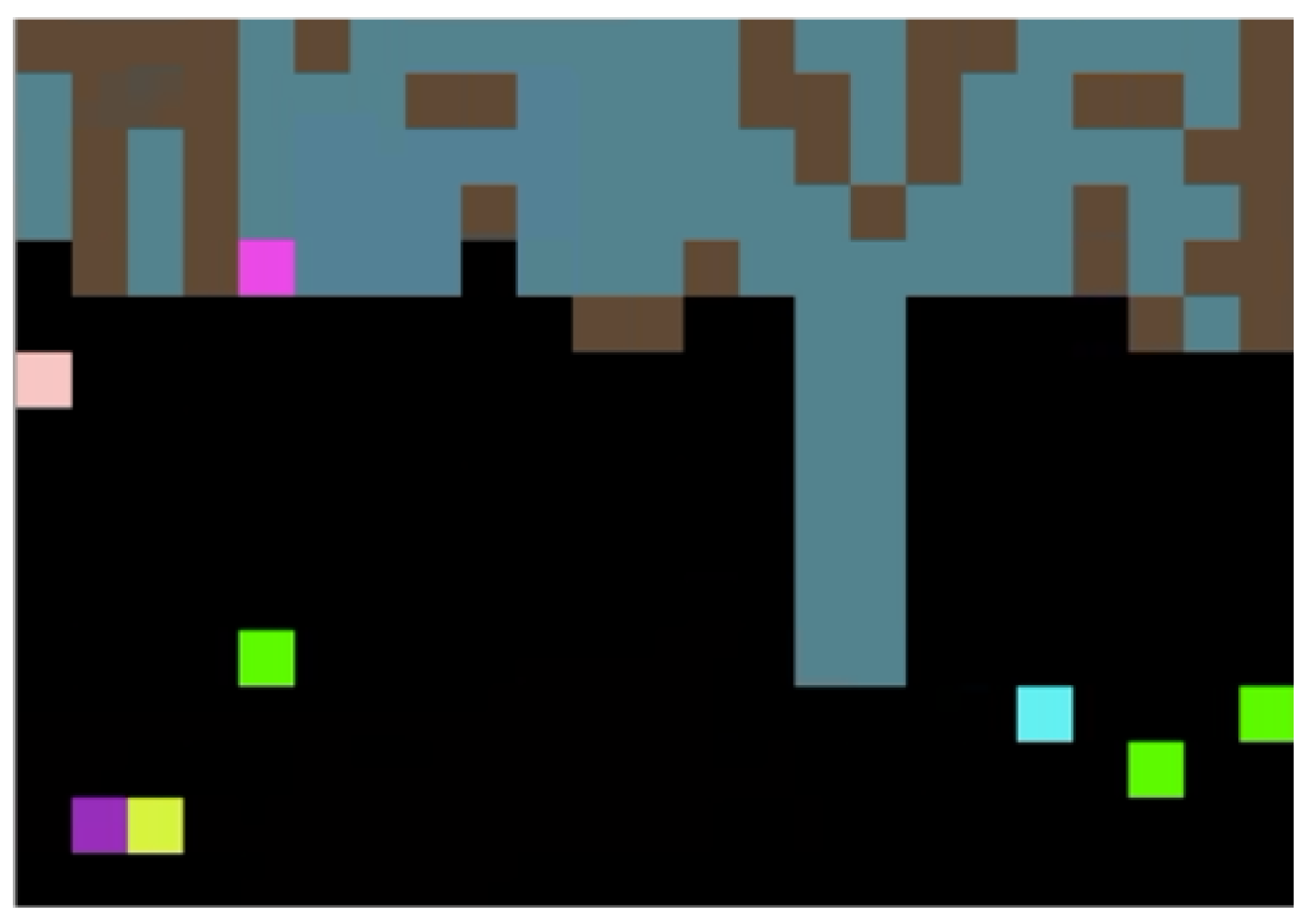
Cleanup: This environment is a rectangular area ($18\times 24$), shown in Figure 2, which includes rivers and flat ground. Among them, the river will produce waste according to a probability, and the amount of waste determines the probability of apples being generated on flat ground. Multiple agents can perform operations on the river and flat ground, including moving (up, down, left, right, and stay), cleaning up the river, and attacking. Apples at the destination will be automatically collected. Cleaning up and attacking operations will make one’s own reward −1. When an agent is attacked, its reward is −50. Therefore, the environment has the following characteristics: apples as the main source of reward, its generation rate is affected by the waste in the river. If we want to get more apples, we must have some agents to clean up the river at the cost of reward −1.

The cost of the agent attacking others (−1) is very small compared to the loss of the attacked agent (−50). However, in a multi-agent system, under the setting of partially observable and independent learning, the agent cannot understand the connection between attacking and being attacked. In order to obtain a higher collective reward, it is necessary to reduce aggressive behavior.

Harvest: This environment is also a rectangular area ($38\times 15$), shown in Figure 3, composed entirely of flat ground. Apples will be produced on flat ground, and the apple’s generation probability is determined by the number of apples around a cell. Agents in this environment behave the same as those in Cleanup, except for cleaning up. The characteristics of this environment are as follows: apples as the main source of reward, their generation rate in a cell is affected by the number of apples around them. The more apples around, the more likely it is to produce apples. Therefore, if the agent collects apples without restriction, no new apples will be produced in the later stage.

Both of these environments reflect social dilemmas: Scenarios when individual interests conflict with collective interests. In order to obtain a higher collective reward in Cleanup, there should be an agent to clean up the river. The same purpose in Harvest, all agents must collect apples in a limited manner. It means that they will understand the huge loss caused by the aggressive behavior and unlimited behavior to the collective reward. Our article tries to realize these targets.

4.2. Baseline

The main algorithms used in this work include IAC, IPPO, and MADDPG. In SSDs, the agent has its own reward function for independent learning. Therefore, we assign the A3C algorithm and PPO algorithm to each agent as a baseline for comparison. Moreover, global information is used in both SR and AEN, so we conducted a control experiment with MADDPG which also applies global information.

The A3C algorithm is an excellent reinforcement learning algorithm that combines the PG algorithm (actor network) and the Q-learning-based algorithm (critic network). Therefore, A3C greatly improves the efficiency of policy learning. Additionally, through multi-environment parallel processing, the sampling rate, and the running speed is increased.

The PPO algorithm is based on the AC architecture (each agent has an actor network and a critic network). However the algorithm realizes the reuse of data through importance sampling. Another innovative point of the algorithm is that it limits the update range of the policy. The PPO determines whether to optimize or not by calculating the relationship between the new policy and the old policy. This idea ensures that each gradient update is in an optimal direction.

MADDPG algorithms are extensions of DDPG in multi-agent systems. The algorithm trains a critical network using global information based on the settings of centralized critic and decentralized policy and predicts their next actions by modeling the policies of other agents. It uses the predicted action to find a self-action that maximizes the joint Q-value. The algorithm has an excellent performance in a multi-agent environment, and has been compared to most RL algorithms as a baseline.

4.3. Experiment Setup

We introduce various hyperparameters settings in detail in this section. In simulation reasoning, the predict length K is 15. There is a CNN network, LSTM network, and fully connected network in the AEN. In the CNN, the convolution kernel size is 6 and the dimensional of the fully connected layer is 64. The times of recurrence is 15 in LSTM. The action contribution evaluation part is a fully connected neural network with two hidden layers of size $128\times 64$. The agent model includes actor network and critic network, and they are also fully connected neural networks. In partial observable environments, the agent’s observation range is $5\times 5$. The discount factor is 0.95. In parallel processing, the batch size is 8000.

4.4. Results and Analysis

The results of the experiment are shown in the figure below. The horizontal axis in the figure represents the training timesteps and the vertical axis represents the collective reward. We use five sets of random seeds to repeat the experiment in two environments. The training duration is various in different environments, but they can fully demonstrate the realization results. We add contribution incrementally based on time, which sometimes leads to the delayed performance of the algorithm.

4.4.1. Cleanup

Figure 4 shows the performance of A3C and PPO algorithms with SR and AEN in the Cleanup environment. The experimental curve clearly shows the improvement effect of our proposed algorithm on the baseline algorithm.

The shaded part in the figure represents the fluctuation of the experimental results of multiple groups. The baseline algorithm in the figures indicates that the collective reward of basic agents can quickly converge to 25 by A3C and 50 by PPO. However, there is no performance improvement after convergence. Without the help of external forces, the agent in Cleanup is caught in a social dilemma: no agent will give up some individual interests for the long-term collective interests. However, after applying SR, the collective reward did not stop at the baseline level, but continued to improve with the passage of training time. After training six million steps, the collective reward of SR-PPO reached an average of about 400, and AEN-PPO reached 800. After training 9 million steps, the collective reward of SR-A3C reached an average of about 125, and AEN-A3C reached about 300.

We know that in the Cleanup environment, if we want to get more resources, there must be agents in the environment to clean up the river. This is not profitable for the individual as they need to lose profit. Therefore, agents that use baselines rarely choose to clean up the river, and are greedy to collect resources. However, after applying SR, agents will choose to clean the river out of consideration for collective interests. The loss of individual interests will be compensated by contributions, thus breaking the social dilemma. The calculation of the contribution in SR is based only on the current trace, which is too limited. The evaluation network in the AEN is constantly updated during the training process.

After referring to more data, the AEN can get a more accurate contribution calculation. Therefore, compared with SR, the performance of the collective reward using the AEN will be superior. Experimental results show that our proposed algorithm breaks the social dilemma by encouraging agents to contribute to the collective.

4.4.2. Harvest

Figure 5 shows the performance of our proposed algorithm in the Harvest. There is no need for an agent to clean up the river in the Harvest, and there are more resources on the map. Therefore, the agent can quickly collect more apples, and the collective reward in the baseline can reach 400. However, because the number of apples in Harvest is determined by the number of apples around it, maintaining a reasonable amount of resources allows one to continue to harvest more resources. The agent that applied SR-A3C and SR-PPO got a collective reward of about 600 after stabilization. The agent that applied AEN-A3C and AEN-PPO got a collective reward of about 800. According to the nature of the Harvest environment, the increase in the upper limit of collective rewards reflects that the agent is indeed acquiring resources in a controlled manner. The experimental results show that our proposed algorithm encourages agent temperance to break social dilemmas.

4.4.3. Discussion

In addition to the comparison with the A3C and PPO algorithms, we also compared the MADDPG algorithm using mutual information. Figure 6 shows the comparison results of A3C-based AEN and MADDPG. In Cleanup, the AEN embodies the advantages of the ultimate collective gain. In Harvest, although the collective returns are not much different, the convergence speed in the early stage is still improved. This demonstrates the effectiveness of the AEN structure for enhancing collective reward and promoting cooperation in the SSDs environment.

Table 1. Maximum collective reward in the two environments.

	A3C	SR-A3C	AEN-A3C	PPO	SR-PPO	AEN-PPO
Cleanup	82	152	378	144	520	1115
Harvest	527	731	813	539	708	922

shows the maximum collective reward of our proposed algorithm in the two environments. We can see that the PPO algorithm using SR and AEN is very significant in the Cleanup environment. Compared to the baseline, there is also a performance improvement. The application of the two algorithms in the two environments also reflects the general applicability of the method we proposed. The method we propose can be applied to a variety of basic algorithms. The intrinsic reward can solve the problem of conflict of interest between individuals and collectives in a multi-agent system.

5. Conclusions

This paper proposes the counterfactual reasoning-based multi-agent reinforcement algorithm to train policy in multi-agent systems. The simulation reasoning method collects data by simulating the environment and modifying actions, then compares with real data to get the continuous contribution of the agent’s actions to the environment. In the action evaluation network, we use CNN and LSTM networks to extract the latent state of the environment. A neural network is used to fit the mapping between joint action and latent state. It also gains a single agent’s continuous contribution to the environment by replacing its action. The continuous contribution of the agent is used as an intrinsic reward, combined with an environmental reward for training. The policy trained in this way will enable the agent to balance individual and collective interests.

Our proposed algorithm has been verified by experiments in SSDs. The comparison with the baseline shows the performance advantage of our proposed algorithm. When facing dilemmas, the interests between the individual and the collective can be balanced by intrinsic rewards based on contributions. In future work, we will continue to optimize the process of extracting latent state in the AEN to obtain a more explanatory latent state and further optimize the evaluation network. Moreover, we will try to combine with hierarchical reinforcement learning to solve higher-level decision-making problems.