Article

On the Black-Box Challenge for Fraud Detection Using Machine Learning (I): Linear Models and Informative Feature Selection

by
Jacobo Chaquet-Ulldemolins
1,
Francisco-Javier Gimeno-Blanes
2,
Santiago Moral-Rubio
3,
Sergio Muñoz-Romero
1,3 and
José-Luis Rojo-Álvarez
1,3,*
1
Department of Signal Theory and Communications, Telematics, and Computing Systems, Universidad Rey Juan Carlos, 28942 Madrid, Spain
2
Department of Signal Theory and Communications, Universidad Miguel Hernández, 03202 Elche, Spain
3
Institute of Data, Complex Networks and Cybersecurity Sciences (DCNC Sciences), Universidad Rey Juan Carlos, 28028 Madrid, Spain
*
Author to whom correspondence should be addressed.
Appl. Sci. 2022, 12(7), 3328; https://doi.org/10.3390/app12073328
Submission received: 28 February 2022 / Revised: 19 March 2022 / Accepted: 21 March 2022 / Published: 25 March 2022
(This article belongs to the Topic Machine and Deep Learning)

Abstract

:
Artificial intelligence (AI) is rapidly shaping the global financial market and its services due to the great competence that it has shown for analysis and modeling in many disciplines. What is especially remarkable is the potential that these techniques could offer to the challenging reality of credit fraud detection (CFD); but it is not easy, even for financial institutions, to keep in strict compliance with non-discriminatory and data protection regulations while extracting all the potential that these powerful new tools can provide to them. This reality effectively restricts nearly all possible AI applications to simple and easy to trace neural networks, preventing more advanced and modern techniques from being applied. The aim of this work was to create a reliable, unbiased, and interpretable methodology to automatically evaluate CFD risk. Therefore, we propose a novel methodology to address the mentioned complexity when applying machine learning (ML) to the CFD problem that uses state-of-the-art algorithms capable of quantifying the information of the variables and their relationships. This approach offers a new form of interpretability to cope with this multifaceted situation. Applied first is a recent published feature selection technique, the informative variable identifier (IVI), which is capable of distinguishing among informative, redundant, and noisy variables. Second, a set of innovative recurrent filters defined in this work are applied, which aim to minimize the training-data bias, namely, the recurrent feature filter (RFF) and the maximally-informative feature filter (MIFF). Finally, the output is classified by using compelling ML techniques, such as gradient boosting, support vector machine, linear discriminant analysis, and linear regression. These defined models were applied both to a synthetic database, for better descriptive modeling and fine tuning, and then to a real database. Our results confirm that our proposal yields valuable interpretability by identifying the informative features’ weights that link original variables with final objectives. Informative features were living beyond one’s means, lack or absence of a transaction trail, and unexpected overdrafts, which are consistent with other published works. Furthermore, we obtained 76% accuracy in CFD, which represents an improvement of more than 4% in the real databases compared to other published works. We conclude that with the use of the presented methodology, we do not only reduce dimensionality, but also improve the accuracy, and trace relationships among input and output features, bringing transparency to the ML reasoning process. The results obtained here were used as a starting point for the companion paper which reports on our extending the interpretability to nonlinear ML architectures.

1. Introduction

Nowadays, most transactions take place online, meaning that credit cards and other payment systems are involved. These methods are convenient both for the companies and for the consumers. In the midst of all this are the banks, which must make sure that all the transactions are legal and non-fraudulent. This is an arduous and complicated task, due to fraudsters always trying to make every fraudulent transaction seem legitimate, which makes fraud detection a very challenging and difficult task [1]. For this reason, banks need to hire skilled software engineers and experts in fraud detection, but they also need to use specialized software, and altogether, it can be very expensive. Traditionally, fraud detection has been based on expert systems [2], which are techniques that solve problems and answers questions within a specific context. The great problem with these expert systems is that the more specialized they are, the more expensive they are to maintain [2]. Artificial intelligence (AI) has the potential to disrupt and redefine the existing financial services industry. In the general context of AI, there is machine learning (ML), which encompasses models for prediction and pattern recognition that require limited human intervention. In the financial services industry, the application of ML methods has the potential to improve outcomes for both businesses and consumers, and it can be a powerful tool against the credit fraud. At present, many works [1,3,4,5] are being devoted to develop ML models against credit fraud. Using ML to generate prediction models can improve efficiency, reduce costs, enhance quality, and raise customer satisfaction [6]. Nevertheless, one of the big challenges and a potentially large obstacle in these models is their lack of transparency in decision making. These models are often black boxes, as we only know their inputs and outputs, but not the processes running inside. This makes them hard to comprehensively understand, and their properties are complicated to validate, so certain forms of risks could go undetected. This type of complexity constitutes a significant barrier to using ML in existing CFD [7,8]. These black boxes have implications for financial supervisors, who will need to take account of the opportunities for enhanced compliance and safety created by ML, and to be aware of the ways that ML could be used to undermine the goals of existing regulations. For example, the United States prohibits discrimination based on several categories, including race, sex, and marital status. Moreover, a lending algorithm could be found in violation of this prohibition even if the algorithm does not directly use any of the prohibited categories, but rather uses data that may be highly correlated with protected categories. The lack of transparency could become an even more difficult problem in the European Union, where the General Data Protection Regulation adopted in 2016 and due to take effect in 2018 gives their citizens the right to receive explanations for decisions based solely on automated processing [9].
Even given this limitation, ML has potential applications in a variety of areas in financial services. The nature of opaque ML imposes significant limits on the use of ML for writing regulations [9]; for example, the U.S. prohibits discrimination on the basis of various categories including race, sex, and marital status [4]. Other of the consequences of black-box models are the potential biases in the results obtained and the difficulties involved in understanding the reasoning processes followed by the algorithms to reach specific conclusions [6,10]. The data used to train the ML models may not be representative in fraud operations [9], thereby risking the recommendation of wrong decisions. Some firms emphasize the need for additional guidance on how to interpret current regulations. Towards breaking down this barrier, the interpretability of these models is fundamental. The regulation authorities are composed by humans, and in this sense the explanations must be understood by humans. In like fashion, the decision models need to be an easily understandable, or in other words, they need to allow us to check which attributes are necessary to produce explanations that are comprehensible [11].
On the one hand, the easiest way to achieve interpretability is to use globally interpretable models, meaning that they have meaningful parameters (and features) from which useful information can be extracted in order to explain predictions [11], such as linear regression or other linear models, including gradient boosting, support vector machines, and linear discriminant analysis. On the other hand, to achieve high accuracy, it is necessary to select the most representative variables for linear models. Hence, the methodology proposed in this present work has as two objectives: first, to reduce the dimensionality while selecting the informative features; and second, to use interpretable models to produce explanations comprehensible to humans. In the companion paper [12], and after different strategies to obtain interpretability in linear models have been developed and compared herein, we present a thoughtful analysis of non-linear models.
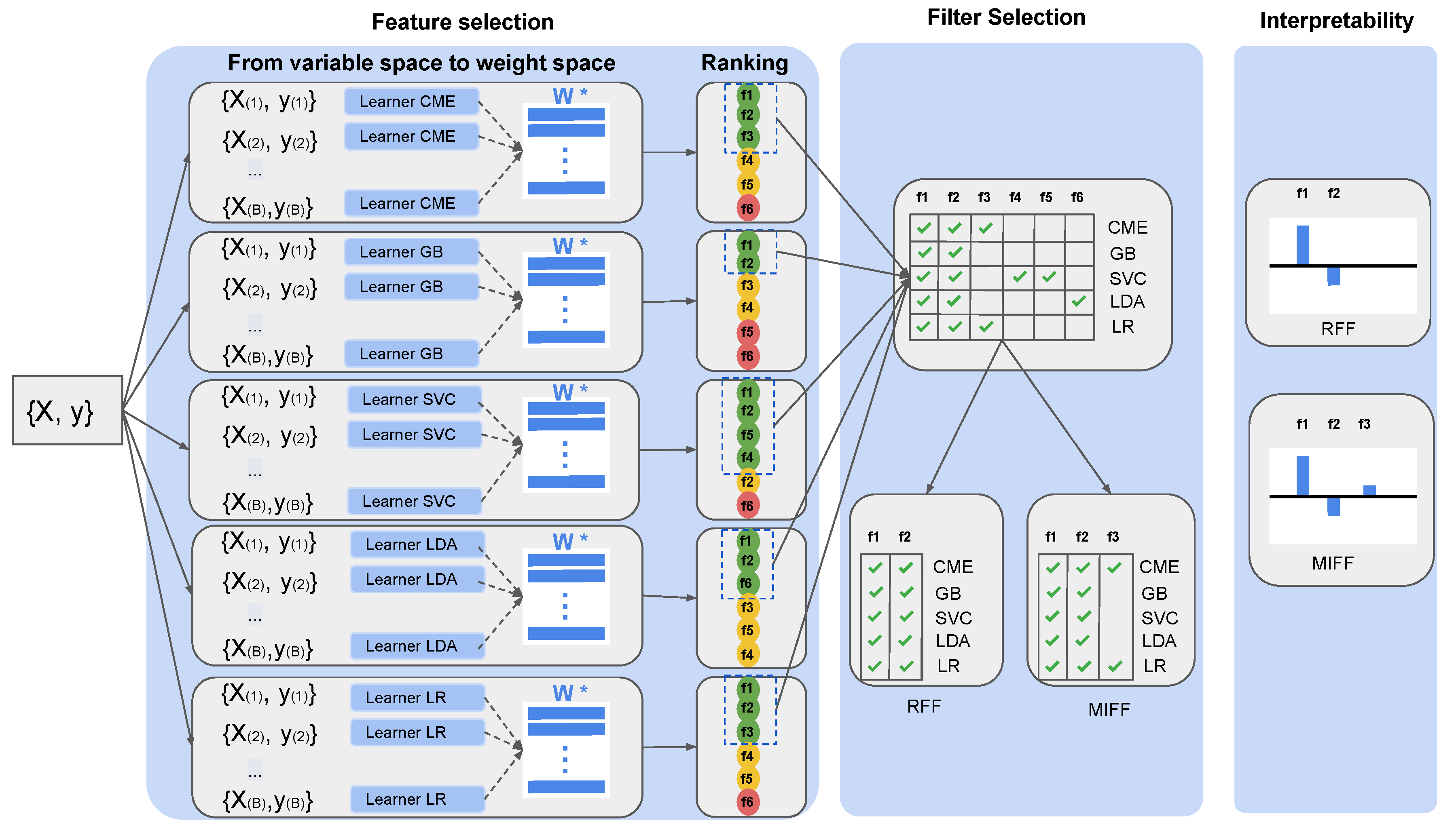
We aimed to create a reliable, unbiased, and interpretable methodology to automatically measure credit fraud detection (CFD) risk. To do so, we emulated a controlled environment using a synthetic dataset that allowed us to propose detailed analysis of all possible variables. The results obtained in this closed and controlled environment, together with the knowledge acquired, allowed us to perform validation on a real database. The proposed methodology incorporates a recently published novel feature selection technique, called informative variable identifier (IVI) [13], which is capable of distinguishing among informative and noisy variables. In the original work, IVI was implemented using only one ML method. We further extended this method and performed intensive benchmarking of a set of different techniques, to extend the method’s validation and to enhance its generalization capabilities in the context of CFD applications. Different subsets of relevant features were obtained as a result of this exploration. We classified them according to newly proposed innovative filters, and to attend to recurrence, according to recurrent feature filter (RFF) and maximally-informative feature filter (MIFF). This reclassification allowed dimensionality reduction: an improvement in accuracy can be obtained as a consequence. In the method, interpretability and traceability are maintained over the process by using linear methods in the matching of each transaction and its corresponding evaluation. Therefore, the contribution of each informative feature obtained in this final model forms a straightforward indication for further legal auditing and regulatory compliance.
This work is organized as follows. A short review of the vast literature in the field of CFD and ML-based systems is presented in Section 2. In Section 3, the IVI algorithm and the RFF and MIFF filters are described in detail. In Section 4, first, the synthetic and the German credit datasets we used are described. Then, we present the qualitative and quantitative benchmarking on synthetic data and a different analysis on a German credit dataset. Finally, in Section 5, discussion and observations are presented and conclusions are stated.

2. Background

In this section, a brief review of the vast literature in the CFD field is presented. Then, we introduce short summaries of state-of-the-art algorithms used in our methodology and their basic equations.

2.1. Related Work

As we have previously introduced, new regulations in CFD have made the auditing and verifiability of decisions mandatory, thereby increasing the demand for the ability to question, understand, and trust ML systems. Consequently, interpretability has become essential to breaking the barrier that is the lack of transparency in ML. The following section presents a summary of relevant works related to these limitations.
ML techniques have a large number of parameters and settings that make them very complex systems. This can often mean that the user of the model is not always able to grasp what knowledge the model has learned from the data so as to make the final decision, thereby leading sometimes to the user’s distrust of these models [8]. In this context, the main challenges for ML applications in CFD are a lack of interpretability and biases (this last one both in data and algorithms) [7].
The first challenge in ML interpretability is the interpretation of the reasons behind a model decision’s in a way that a human can understand [8]. In financial services, firms have great challenges in meeting regulatory requirements to explain decision making when using black-box models. The regulation should not be considered as an unjustified barrier to ML deployment, but some firms emphasize the need for additional guidance on how to interpret current regulations [7]. Current works rely on naturally interpretable models, for instance, linear models [11]. With models of this kind, it is easy to understand the predictions by just scrutinizing the weights for each feature in the model. Other relevant work [14] is focused on local surrogate models, such as local interpretable model-agnostic explanations (LIME). Said surrogate models are trained to approximate the predictions of the underlying black-box models. Instead of training a global surrogate model, LIME focuses on training local models to explain individual predictions. A model with 100% accuracy cannot be used if the decision process cannot be explained. In this context, some interesting works have started questioning the cost of interpretability and how this interpretability affects predictive accuracy [15].
The next challenge in black boxes consequences is biases. ML algorithms in many cases operate by seeking correlations that try to maximize the predictive power. However, the use of ML in financial services also raises several potential problems, given that the data used to train the ML algorithms may not be representative data for the problem [9]. In some cases, this can produce results based on spurious relationships and thus lead to biased conclusions being drawn [6]. In spite of training these models with enough data, the algorithms can become more ingrained, and previously unforeseen risks are appearing, including the risk that a perfectly well-intentioned algorithm may inadvertently generate biased conclusions that discriminate against protected classes of people [16]. Algorithms often do not distinguish causation from correlation, or they do not know when it is necessary to gather additional data to form a sound conclusion, and for those reasons it is crucial to obtain interpretability for ML models applied to financial services. Interesting works are currently underway that are developing techniques to detect the biases of these algorithms [14,15,17]. In order to improve the accuracy in ML algorithms and to provide interpretability while reducing biases, the so-called feature selection stage is crucial. As the data multiply, the quality of data required for processing ML algorithms decreases gradually, an effect that has long been known as the curse of dimensionality [18,19]. Higher dimensional data lead to the existence of noisy, irrelevant, and redundant data, which in turn cause overfitting of the model and increase the error rate of the learning algorithm. To handle these problems, techniques of dimensionality reduction can be applied. One set of them is feature selection (FS), which is broadly used to clean up the noisy, redundant, and irrelevant data [20]. The use of FS can improve the accuracy, efficiency, applicability, and understandability of a learning process. For this reason, many methods of automatic FS have been developed. In FS, a subset of features is selected from the original set of features based on feature redundancy and relevance. We can classify feature subsets as four types according to [21], as follows: (1) noisy and irrelevant; (2) redundant and weakly relevant; (3) weakly relevant and non-redundant; (4) strongly relevant. Some of the popular approaches to classify the features in these types are filter methods, wrapper methods, and embedded methods. Filter methods analyze the usefulness of each feature by using relevance techniques, mainly from hypothesis tests or mutual information estimations [22], and they work independently from the used classifier. Wrapper methods, such as forward feature selection and backward feature selection [23], solve ML problems to assess the relevance of each feature in the input space [24]. They use a ranking procedure that allows us to remove low-scoring features. These methods are found to be fast, scalable, computationally simple, and independent of the classifier. Finally, embedded methods, such as recursive feature elimination (RFE) [25], aim to increase their efficiency by combining the FS procedure with training a subsequent learning machine. Many of the embedded methods impose regularization on the solution. Recent works have proposed a novel FS method, known as IVI [13], which is capable of identifying the informative, the redundant, and the noisy variables. It transforms the input-variable space distribution into a coefficient-feature space by using existing linear classifiers or efficient weight generators, and it has been shown to provide improved performance and interpretability compared with classical methods and with the RFE criterion.

2.2. State-of-the-Art Algorithms

CFD strategies have existed since the late 1990s and initially relied on expert driven technologies. In recent times, ML has predominated, as these new techniques offer better results in terms of accuracy [1,2,3,6]. Good examples of these techniques are linear classifiers, which allow us to transform the input space into the weights space. This strategy links the contributions of the input variables to the result in a traceable way, offering direct interpretability of the final outcome [13].
In the following paragraphs, we summarize the linear ML algorithms we evaluated in this work, but let us first introduce the notation to be used throughout the paper. Let X R N × L be the input data matrix containing the input set of vectors in rows, with N observations of L features, where x n is a column vector with L features for n = 1 , , N . We consider a classification problem with a binary output variable grouped in vector y R N , such that y l ϵ 1 , + 1 for n = 1 , , N . The relationship among each input feature and the output class is represented by the feature weights in vector w learned by a linear classifier method so that y n = w T x n + b represents the discriminant function, and the sign of y l can be used as the decision output.
Linear regression (LR) models the relationship between multiple input variables by fitting them through a linear equation. One variable is considered a dependent variable ( y n ), and the other variables x n are considered to be explanatory variables [26]. In general terms, this relationship may not hold for the whole sample base, and so a noise term or error terms need to be added to the mathematical formulation ( ε ). We can describe the underlying relationship with the following equation:
y l = w T x n + b + ε l
Linear discriminant analysis (LDA) is a generalization of Fisher’s linear discriminant [27]. LDA is able to find a linear combination of features characterizing two or more sets with classification purposes, and for dimensionality reduction previous to subsequent classification. The main difference between LR and LDA is that LR analysis deals with a continuous dependent variable, whereas LDA must have a discrete dependent variable. LDA aims to represent a single dependent variable as a linear combination of others. Given two classes of multidimensional observations, with means m 0 , m 1 and covariances Σ 0 , Σ 1 , the linear combination of features w T x has mean w T m i and variance w T Σ i w , for i = 0 , 1 . The separation between these two distributions can be defined as the ratio of the variance between the classes to the variance within the classes, i.e.,
S = σ b 2 σ w 2 = w T m 1 m 0 2 w T Σ 1 + Σ 0 w
where σ b 2 represent the variances between the classes and σ w 2 represent the variances within the classes. It can be shown that the maximum separation happens when
w = c Σ 0 + Σ 1 1 m 1 m 0
where c is a constant. When LDA assumptions are fulfilled, this is equivalent to LDA equations. For high-dimensional input feature spaces with highly correlated covariates, this algorithm also can exhibit some instability; hence, we often regularize the matrix inversion and use the following equation:
w = c Σ 0 + Σ 1 + λ I 1 m 1 m 0
where λ is the regularization parameter, and I is the identity matrix.
Support Vector Machines (SVM). Conventional ML classifiers are strongly affected by the high dimensionality of the features observation vectors, and they tend to overfit to the data in the presence of noise, or to perform poorly with few training samples. In the last few years, the use of SVM [28,29] for ML practical applications has received wide attention. SVM are supervised learning models with associated learning algorithms that analyze data used for classification (SVC) and regression (SVR) analysis. SVM constructs a hyperplane or set of hyperplanes in a high or infinitely dimensional space. Intuitively, good separation is achieved by the hyperplane that has the largest distance to the nearest training data-point of any class, since in general the larger the margin, the better the generalization error of the classifier [30,31]. In contrast to previous ML algorithms, SVM maps the input vector to a higher-dimensional space. SVM can solve linear and non-linear problems, and works well for many practical problems. For this work we have used a linear kernel. We want to find the maximum-margin hyper plane that divides the group of points x k , for which y k = 1 from the group of points x m , for which y m = 1 . Given a nonlinear mapping ϕ · , the SVM method solves:
min w , b , β l , ρ 1 2 w 2 + C i β l
In consideration of
y l ϕ x l , w + b 1 β l , l = 1 L
where w and b define a linear classifier in the feature space and β are positive slack variables enabling one to deal with permitted errors. The appropriate choice of nonlinear mapping ϕ guarantees that the transformed samples are more likely to be linearly separable in the feature space. Equation (5) is solved by using its dual problem counterpart, yielding w = l = 1 L y l α l ϕ x l , and the decision function for any test vector x is finally given by
f x = s g n l = 1 L y l α l K x l , x + b
where α l are Lagrange multipliers corresponding to constraints in Equation (5), those training samples x l with α l 0 being vectors; the bias term b is calculated by using the unbounded Langrange multipliers; and K represents the Mercer Kernels used to handle the nonlinear algorithm implementations.
Gradient Boosting (GB) is an ML technique for regression and classification problems that produces a prediction model in the form of an ensemble of weak prediction models. It builds the model in a stage-wise fashion, and it generalizes the models by allowing optimization of an arbitrary differentiable loss function [32,33,34]. The goal is to find an approximation F ^ ( x ) to a function F ( x ) that minimizes the expected value of some specified loss function L ( y , F ( x ) ) ; that is,
F ^ = arg min F E X , y [ L ( y , F ( X ) ) ]
The GB method assumes a real-valued y and seeks an approximated F ^ ( X ) in the form of a weighted sum of functions h m ( x ) called base (or weak) learners, in such a way that
F ^ ( x ) = m = 1 M γ i h i ( x ) + c
where M is the number of weak models being used.

3. Materials and Methods

This section describes the fundamentals of the methodology implemented. To do so, we present next some details of the IVI algorithm and how it is used. This methodology was built on the initial hypothesis that interpretability can be obtained based on the importance of the features. With this in mind, we reflected the contribution of each feature in the decision process by calculating its weights in different ML methods and consolidating these contributions. Once we selected the feature contributions, we developed two kinds of filters with the aim of avoiding bias and to obtain a more comprehensive view of the adjusted data models. The rest of the section describes in detail each of these steps.

3.1. Informative Variable Identifier

In our proposal we use a recently proposed FS method called IVI [13], which is capable of identifying the informative, redundant, and noisy variables. It transforms the input-variable space distribution into a coefficient-feature space by using existing linear classifiers or a more efficient weight generator. Informative features and their relationships are determined by analyzing the joint distribution of these coefficients with resampling techniques. IVI selects the informative variables and then it passes them on to some linear or nonlinear classifier. Experiments have shown that IVI can outperform state-of-the-art algorithms in terms of feature identification capabilities, and even in classification performance when subsequent classifiers are used. The IVI algorithm is built on the initial hypothesis that weights, w , learned by a linear classifier method, y l = w T x l + b , are capable of summarizing the relationship between each feature. The IVI algorithm introduced in the original work [13] was implemented with the covariance multiplication estimator (CME) as a weight generation method designed to be competitive with the standard linear algorithms. CME is a low-computational-cost weight generator which is built on the relationships among input features, and on the relationships between input and output variables. Given an input dataset and a class variable, { X , y } , where X R N × L is the input data matrix, containing the input set of vectors in rows, with N samples or observations of L features and y 1 , + 1 . C X X and C X y , denote the sample covariance matrices estimated as
C X X = 1 N X T X R L × L
C X y = 1 N X T y R L × 1
The l-dimensional coefficient vector of CME is defined as follows:
w = s i g n C X X g 1 C X X g C X y
where ⊙ denotes the Hadamard product or element-wise product, and g is the integer exponent of the element-wise power. Through the use of the IVI algorithm, we selected different groups of relevant features. The IVI algorithm consists of three stages that can be summarized as follows.
The first step of the IVI algorithm consists of estimating the statistical distribution of the weights learned by a given criterion for each input feature. For this purpose, we transformed the input-feature space into a weight space by resampling the dataset and computing one set of weights for each input feature, and this transformation is summarized in Algorithm 1. Resampling techniques were used: every group of samples was trained with a linear model (CME), which provided us with an estimation of the empirical distribution of any statistical magnitude that can be built computationally. We sampled N g rows in X and y to get the b t h resampling X b , y b . For every resample, we estimated the statistical magnitude of interest which, in our case, was the weight vector w ( b ) . By repeating this procedure B times, we got an estimate of the marginal empirical distribution:
f ^ w w = 1 B b = 1 B δ w w ( b )
where δ ( w ) denotes the usual Dirac’s delta function. The results of the first step of the IVI algorithm are the feature weights which were then used to identify feature relevance and redundancy in Algorithm 1.
Algorithm 1 IVI-Algorithm Step 1.
Require: 
Training set X and y , and number of resamples, B.
Ensure: 
Resampled weight matrix, W R B × L .
1:
forb← 1 to B do
2:
   Generate a random subset of the training set X ( b ) and y ( b ) , with size L b .
3:
   Calculate the weight vector w ( b ) using X ( b ) and y ( b ) as training dataset.
4:
   Save vector with the weights w ( b ) in the bth column of matrix W .
5:
end for
In the second step, the statistical properties of the marginal distributions of the weights were used to identify the informative features and group together those found to be mutually redundant. This is summarized in Algorithm 2. Furthermore, IVI identified the informative and the redundant features by discovering the statistical properties of the weights. The former was carried out through the analysis of the confidence intervals of the resampled weights associated with every input feature. The correlations of weights were then used to locate and group mutually redundant features. Now, with these disjoint groups, informative features could be discerned from the noisy one. We selected only the informative disjoint groups. To do this, the informative groups were considered to be disjoint groups with at least one feature identified. Thus, groups of features that shared information but did not contain any relevant one were discarded, and all those features could be considered noisy. The algorithm to calculate the threshold and the groups of redundant features is summarized in Algorithm 3.
Algorithm 2 The IVI algorithm, step 2. Confidence intervals to identify relevant features.
Require: 
Weight matrix W and level of confidence for significance tests, α .
Ensure: 
Features labeled as relevant
1:
Use W to construct confidence intervals at α level.
2:
Store the list of features with confidence intervals that do not overlap zero and label them as relevant.
Algorithm 3 The IVI algorithm, step 2.2. Identification of feature redundancy.
Require: 
Resampled the weights matrix, W R B × L ; number of folds, k, to calculate the threshold.
Ensure: 
Threshold to identify redundant features, p t h , and disjoint groups.
1:
Split the set W into k subsets, W i , with i = 1 , , k .
2:
forl, m l m ← 1 to N do
3:   
Calculate the absolute value of the Pearson correlation coefficient of the B resampled weights of features l and m in W and save consecutively in vector p W .
4:   
For each fold, calculate the absolute value of the Pearson correlation coefficient of the features l and m in W i , yielding p W i .
5:
end for
6:
Save the average of the p W i in vector p ¯ W k
7:
Sort p W and p ¯ W k in descending order by p W .
8:
Compute the cumulative difference between p ¯ W k and p W , and look up the row containing the minimum cumulative difference. Define the threshold, p t h , as the correlation store in row r t h of vector p t h fulfilling
r t h = arg min r i = 1 r p ¯ W , i k p W , i
9:
Redundant features are defined as features pairs with correlations weights higher than the threshold.
The last step is a ranking of features created in descending order of importance. For this, we needed first to order in descending importance the features in each of the disjoint groups obtained with IVI. Some groups contained more than one relevant feature. We separated such groups into subgroups that included only one relevant feature each and its most direct redundant relation. Finally, the resulting groups and subgroups were ordered to produce the final ranking. Finding the relevant features in the disjoint groups identified by IVI was the first task. To do that, an importance measure was used: I m p l , which was calculated for each feature l as the absolute value of the average weight across replicates and divided by the square of the range of the 95% confidence interval of the resampled weights; that is,
I m p l = | m e a n ( W l ) | w l h , w l n , 2 , l ϵ I
where w l h , is the value for upper interval, w l n , corresponds to the lower interval, and I is a set of informative features. When a disjoint group contains only two features, the highest importance determined the most relevant feature in the group. The other feature were taken as redundant versions of the former. For larger groups, there can be more than one relevant feature. To find them out, we explored the complete set of subgroups of features that we would get if we increased the weight correlation threshold used to build the initial disjoint group. Next, we defined the importance of a (sub)group of features G as the absolute value of the sum of the importance of the features in the group. As a result, groups or subgroups with sum of importance well above 1 were likely to include more than one relevant feature. On the contrary, not very informative subgroups with no relevant features were expected to have sum of importance well below 1. Subgroups with only one relevant feature were expected to get sum of importance close to 1. Therefore, for each initial disjoint group, we selected the subgroups configuration yielding the lowest sums of subgroup importance. Each of these subgroups contained one relevant feature and its redundant copy. Finally, the resulting groups and subgroups of features had to be ranked. We used a different importance measure which places more weight on the dispersion of the estimates of the coefficients of the features. Each feature importance was calculated and then normalized by dividing it by the maximum importance. The groups of features were ordered by taking into account the sum of their importances. The final ranking of features builds on this group ordering to show first the relevant features in each informative (sub)group, and then, following the same group-importance descending order, the redundant features.

3.2. Methodology to Achieve Interpretability

In this work, we aimed to create a reliable, unbiased, and interpretable methodology to automatically measure CFD risk. In this sense, the proposed methodology involves three steps. The entire system flow of the proposed model is shown in Figure 1. This methodology is sequentially described step by step as follows.
  • Step 1: FS Extraction. Extract common informative features by applying the IVI algorithm.
  • Step 2: FS Filtration.
  • Step 3: Interpretability based on features’ weights.
The first step of this methodology consists of an FS stage that allows us to find the relevant features and to reduce the noise in the data models. As noted earlier, we use IVI [13], which is capable of identifying the most relevant features. The IVI algorithm introduced in the original work was implemented with CME as a weight generating method designed to be fast with the standard linear algorithms. In our methodology, we have expanded the weight generator using different classification algorithms. Our underlying rational to this approach is twofold. On the one hand, we aimed to obtain a more comprehensive view of the problem, due to the fact that each algorithm yields its own specific properties. On the other hand, the features that have been selected in multiple algorithms are more consistent. For this purpose, in this work we included SVM, LDA, LR, and GB in addition to CME. All these methods are linear. The algorithm to obtain the relevant features for each ML algorithms is shown as Algorithm 4.
Algorithm 4 Methodology, step 1.
Require: 
Training set X and y and ML Algorithms
Ensure: 
Relevant features for each ML Algorithm
1:
Initialize all the ML Algorithms V = CME , GB , SVC , LDA , LR
2:
Initialize vector with features selected F S ( v ) = { } ; v s . V
3:
for all a l g V do
4:
 Execute IVI Algorithm using a l g
5:
 Obtain the vector with relevant features, f r
6:
F S ( a l g ) = f r
7:
end for
The second step of our methodology is focused on reducing bias and obtaining a global view of the problem. To do this, we have developed a filtration process due to FS sometimes or often having two biases. Namely, on the one hand, biases based in dependence on general characteristics of the training data, and on the other, biases based on the ML algorithms used. Using the IVI algorithm, we performed resampling of the data to train ML algorithms, and in this sense, we minimized the training data bias. In the case of ML algorithm bias, we have obtained the FS with different ML algorithms (namely, SVM, LDA, LR, and GB, in addition to CME). The next step was to find which of these features are truly informative in all cases. For that purpose, the features needed to be subjected to a filtration process, at the end of which, only the features that were consistent were included in our model. We have established two kinds of filter for relevant features in IVI, to leave aside the redundant and noisy features:
  • Recurrent Features Filter (RFF): We accepted those feature that were selected consistently in every single ML algorithms application using IVI. This filter was very restrictive, targeting only the most representative features, forcing an aggressive reduction in dimensionality, and achieving the highest accuracy in a fast way.
  • Maximally-informative Features Filter (MIFF): We considered those features that were at least selected in two of the ML algorithms used. This filter is less restrictive and caused a moderate dimensionality reduction compared with the RFF. In contrast, this filter was able to identify relationships among features that provided higher prediction accuracy.
Finally, the last step in our methodology focuses on the interpretability on the problem. ML-based linear classifiers can be seen as transformers of the space of the input variables to the space of the weights assigned to each of these features. Those weights actually summarize the contributions of the features in the decision process and the interplay among input and output data in the context of the particular classification problem under study. With this in mind, we used the features selected in MIFF and RFF to obtain a more comprehensive view of the problem, and we again trained the ML models with linear models. The weights assigned to features showed us the importance of each feature. This is shown in Algorithm 5.
Algorithm 5 Methodology, step 3.
Require: 
Training set X and y and ML Algorithms
Ensure: 
Features selected in MIFF and RFF filters
1:
Initialize all features selected V F S = FS M I F F , FS R F F
2:
Initialize all the ML Algorithms V = CME , GB , SVC , LDA , LR
3:
for all a l g V do
4:
for all f s V F S do
5:
  Train linear ML a l g with f s
6:
  Obtain the weights of each f s
7:
end for
8:
end for

4. Experiments and Results

In this work, we propose a novel methodology to simultaneously face the double challenge of applying new, powerful, and proven AI tools, while maintaining the interpretability of the underlying descriptors, thereby allowing compliance with the rigorous regulations of data protection and non-discrimination in force for financial institutions. The developed methodology helps the interpretable linear methods by capturing the relevant features and leaving aside the black boxes, while minimizing the potential bias. To do so, experiments for both synthetic and real data were performed as follows. First, we compared a number of the ML methods with the IVI technique in order to evaluate their capacities for automatic classification. Second, we modeled different learning architectures that allowed us to evaluate the predictive value of the result (CFD), using various sets and subsets of features. This second analysis offers a quantified vision of the predictive capacities of the method–features pairs, to adequately qualify the different options. Third, a detailed evaluation of the incremental predicted value was performed for each of the previously defined methods. We analyzed them feature by feature, along with the speed of convergence and the predictive capacity of each. A final exercise in the analysis of the coefficients, applied to each of the features in the different methods, allowed us to assess the contributions (interpretability) of the different features to the final predictions.
This section is divided into two main subsections presenting the experiments on the synthetic and real datasets. Prior to the experiments, the datasets are introduced. The general strategy guiding the experimentation was to scrutinize and fine-tune the synthetic dataset to validate the methodology, for later evaluation of the generalization capabilities to actual CFD cases in the real dataset.

4.1. Datasets

Although there are a large number of articles published about CFDs, it is not easy to access the actual data used due to data protection and confidentiality restrictions. That is why in this work, initial analysis has been prepared using surrogate signals generated by the authors, which helped us to define and model the detailed study to be carried out. This analysis process based on synthetic signals offered the required flexibility to evaluate the predictive capacity of the different variables, thanks to the effective knowledge provided by having built it. The knowledge acquired during this process allowed us to subsequently analyze the eventual generalization on the real dataset. For this last step, we used the database provided by Strathclyde University [35].
Synthetic Dataset. The first dataset introduces a synthetic linear classification problem with a binary output variable, and it was developed for the original proposal of the IVI algorithm [13]. It has 485 input features. In this work, and for reasons of representability and execution time, we have used a subset of features while keeping the feature names. The dataset used here included a set of 23 input features distributed as follows: 11 input features were drawn from a normal distribution, and 5 of them were used to linearly generate a binary output variable, specifically f 0 , f 1 , f 2 , f 3 , and f 4 . Therefore, these five features are informative for the problem. A set of another 12 features were randomly created with no relation to the previous ones, so that they could be considered as noisy and non-informative variables. Additionally, a new group of six variables were computed as redundant with the informative input features.
German Credit Dataset. This repository is known as the German credit fraud (Stattog) [35], and it contains real data used to evaluate credit applications in Germany. We used a version of this dataset that was produced by Strathclyde University. The German credit dataset contains information on 1000 loan applicants. Each applicant is described by a set of 20 different features. Among these 20 features, 17 of them are categorical and three are continuous. All these features are commonly used in CFDs, and some examples are: credit purpose, savings, present employment, and credit amount. There are no missing values. To facilitate FS and in order to train the models, the values of the three continuous attributes were normalized, and for the discrete features, they were converted to one-hot encoding. After these pre-processing stages, the final dataset was 61-dimensional.

4.2. Analyzing the Synthetic Dataset

As we introduced earlier, we first applied the novel FS strategy based on the IVI algorithm to identify the relevant features. This effort was intensively executed by the five different algorithms introduced earlier, namely, CME, SVC, GB, LR, and LDA. This approach allowed us to achieve a more unbiased perspective of the real effective potential of selected features, and of the sustainability and consistency across methods. 
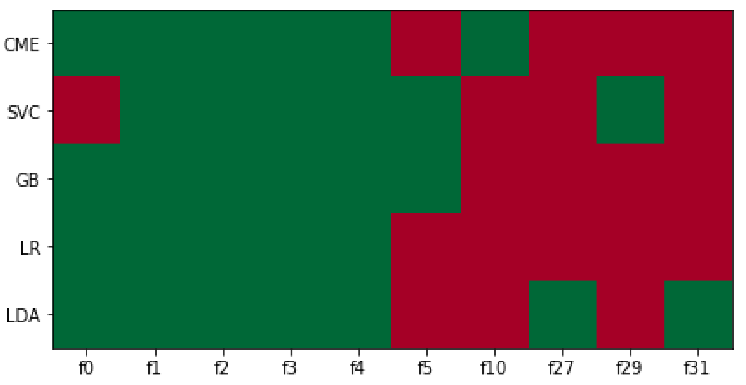
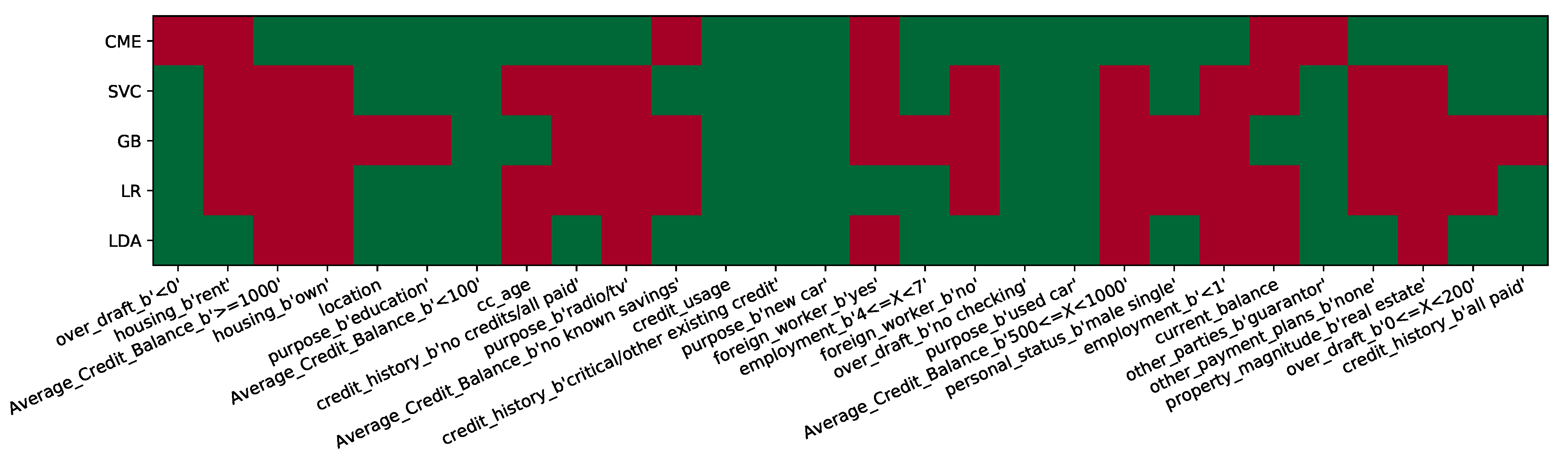
Figure 2 summarizes the outcome of the IVI algorithm for each individual ML technique. In this figure, validated selected features (columns) are in green and those ones not identified as significant by the algorithm (rows) are in red.
We should recall at this point that features identified as relevant for all ML methods were classified as categorized as RFF, as they recurrently and consistently were relevant in all methods. Features f 1 f 4 were all included in this set, but f0 was not identified as such due to the miss-classification by SVC. In the same vein, features identified as relevant for at least two methods were understood to be informative for further analysis and so were chosen for the MIFF group of variables. For this specific case, features f 0 f 5 met the MIFF criteria and were included as members of this filter. These features perfectly match with the relevant features on the synthetic dataset ( f 0 f 4 ), other than one redundant feature ( f 5 ). Attending to these results, we can conclude that the IVI algorithm was consistent with the different ML methods, so it appears to have a valid feature selection ability.
In an attempt to verify and quantify the results, accuracy was calculated in sixteen different scenarios, for SVC, GB, LR, and LDA, and considering different sets of features, namely: (i) all the available features; (ii) only the relevant features according to IVI for each corresponding ML method; (iii) MIFF-classified features; (iv) RFF-classified features. CME was not considered for this task, as CME is a fast weight-generator method but is not a classifier. Table 1 summarizes the means and standard deviations of the 100 resampling executions for 16 different scenarios. This table shows how the accuracy remained mostly invariant among all the classification methods, as the different columns reflect almost no change in terms of mean or standard deviation. The only exception can be found in the case of GB, which in all cases, still shows a smaller classification capability to the rest of the analyzed methods. Similarly, in the case of LDA, when applied to all the available variables, a slight reduction in its prediction capacity can be appreciated. The benchmark illustrates that the best results were obtained when the MIFF filter was used, and there was equivalent predictive power when all the variables were used, reaching in both cases the predictive accuracy of 98.8%. The standard deviation was in all cases lower than 4%. The IVI model offered in all cases, very similar results to the outstanding methods (97% accuracy). On the contrary, the RFF filtering suffered in its predictive capacity compared to the rest of the models, showing the lack of expressive power (90% accuracy) due to the non-incorporation of variables as a consequence of the incorrect classification of relevant variables.
As a general result of the analysis, we can recall that although we focused on a limited number of families of ML linear algorithms, each of them treated independently revealed equivalent performance, and the accuracy was tightly related to the features incorporated as input variables. These results indicates two separate, relevant ideas: (i) the importance of FS as a key element for the performance of the ML model; (ii) the limited relationship among accuracy and the ML method that is chosen provides the possibility of picking the method based on its computational efficiency without leaving out any potential expressive capacity.
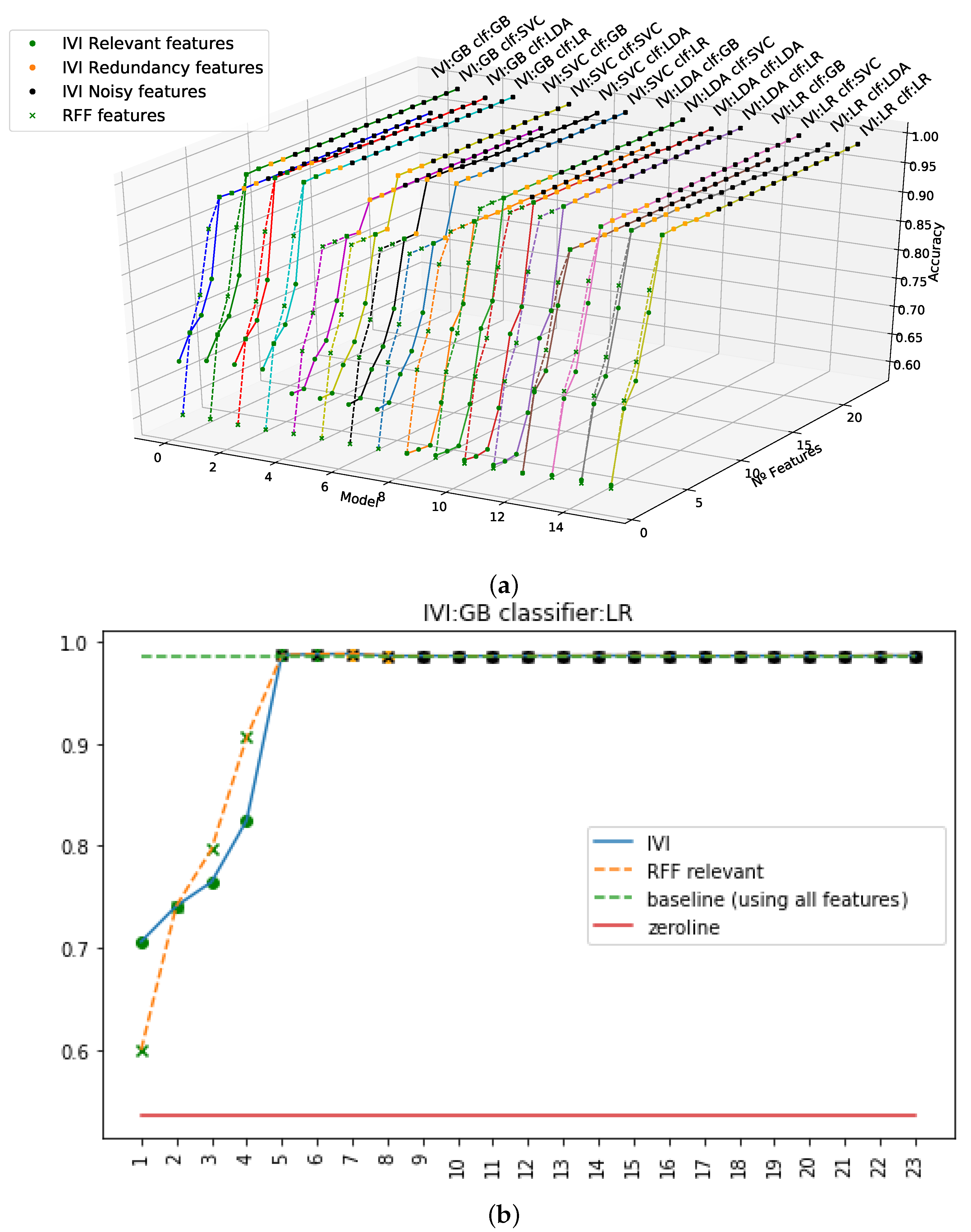
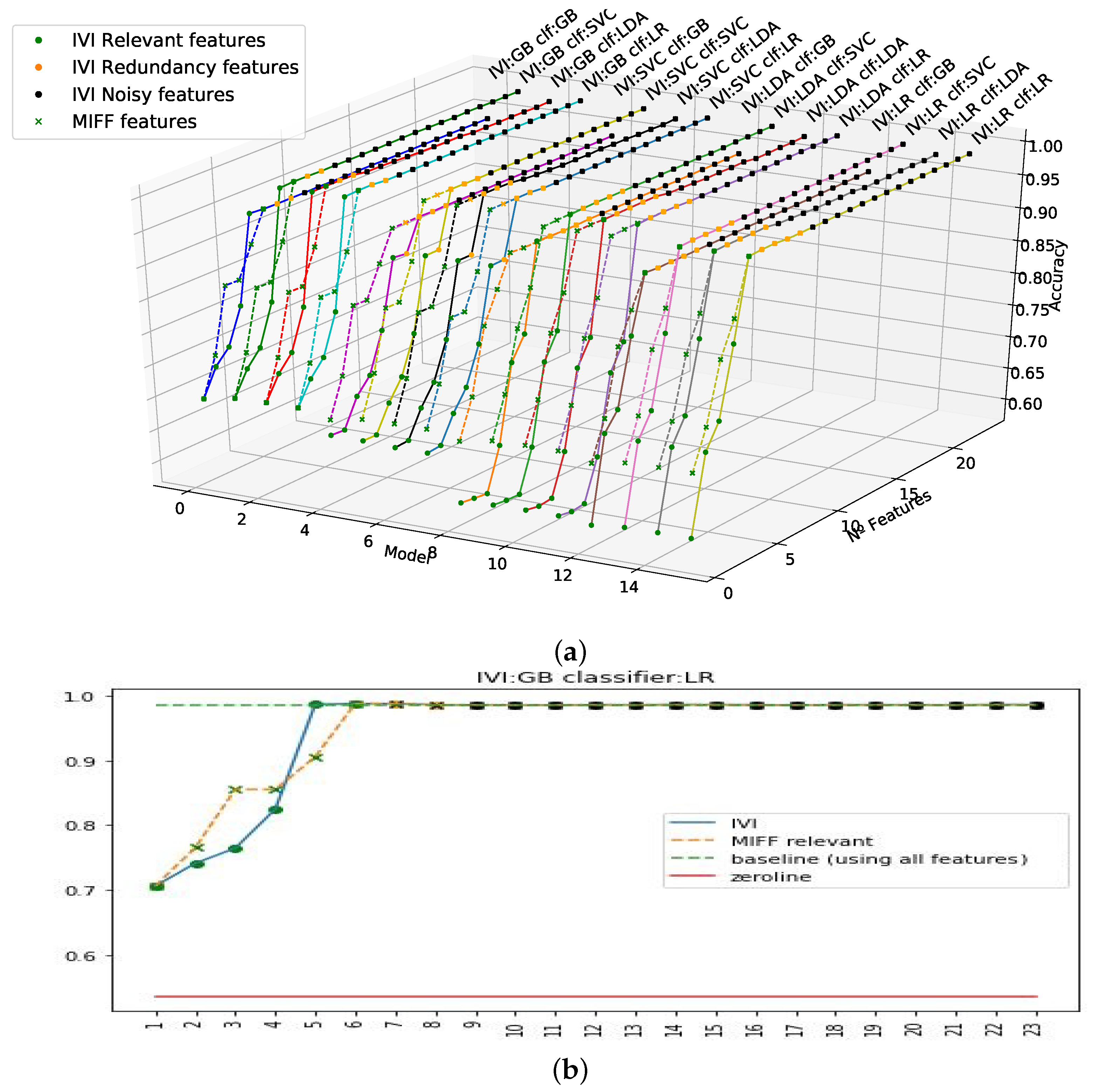
The results obtained in previous experiments suggested the need for a greater and in-depth analysis of both the FS techniques and the variables themselves, for a better understanding of the underlying dynamics. To do so, a number of experiments were conducted considering all variables, for both filters (RFF and MIFF). Experiments were designed in a way to visualize the contribution of each variable by incrementally adding features on a one-by-one basis.
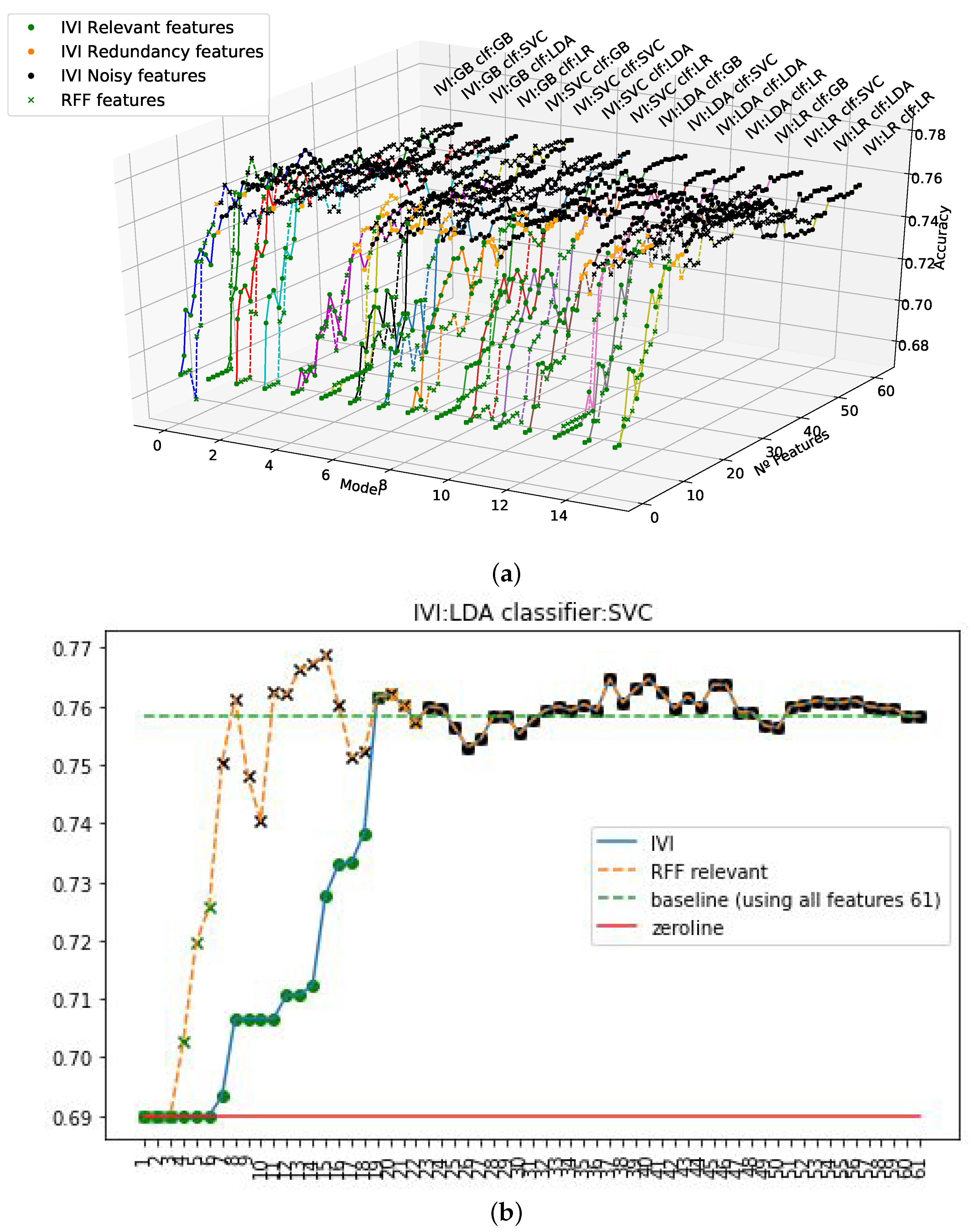
 Figure 3 and 
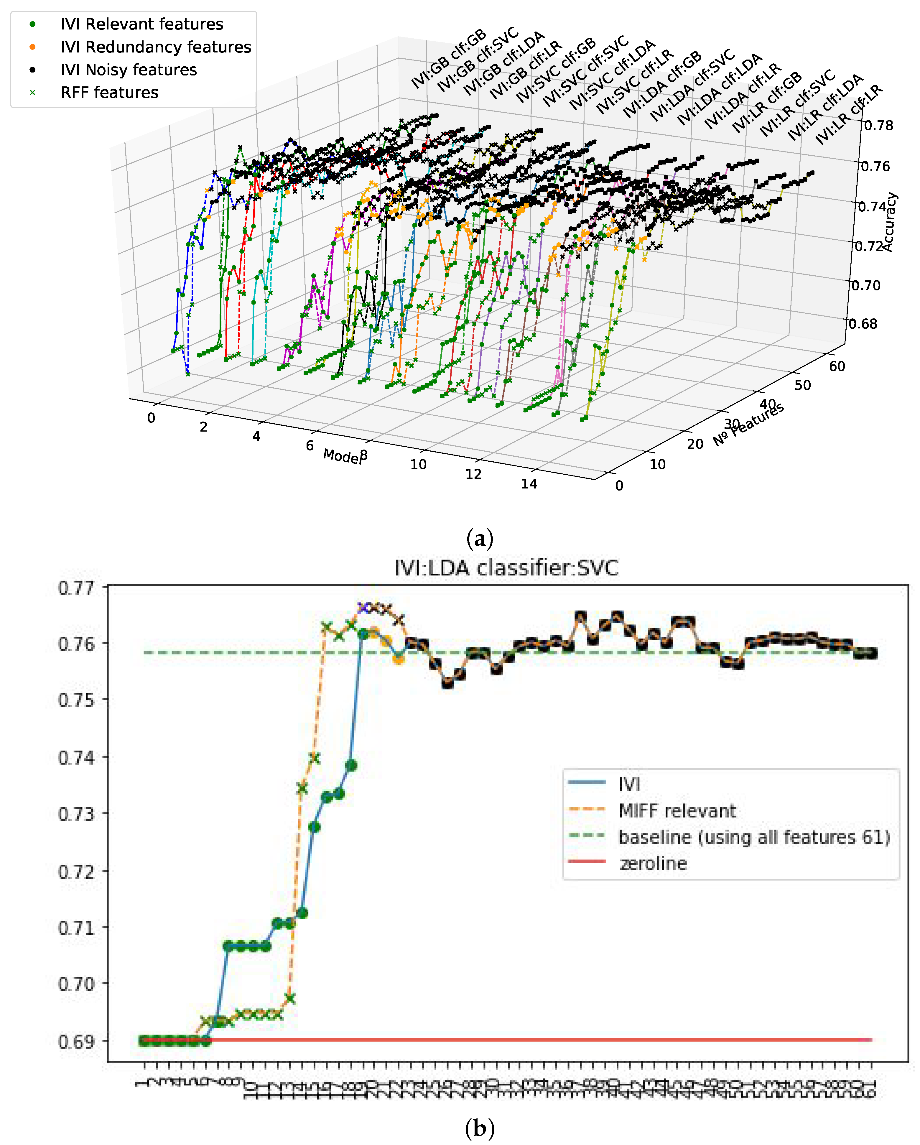
Figure 4 represent the resultsof the corresponding experiments. In the experiments, the variables were added up in sequential order according to their relevance, starting with the most relevant one as defined by the IVI method. Figure 3a presents the evolution of the sequential results for all the experiments when applying the RFF filter, and Figure 4a shows the results of applying the MIFF filtering, both in an M-mode presentation (3D perspective) and in a profile representation. The plots represent two scenarios for each method, as a continuous lines depicts the corresponding results for the standard IVI representation, and the overlaid dotted line follows the process using the RFF or MIFF filtering. IVI standard features were incorporated in the incremental feature experiments in order of relevance (specifically, first informative, then redundant, and finally, noisy). As only filtered features were chosen for RFF and MIFF, the remaining components were added according to standard IVI sequence to complete the full feature set. In Figure 3 and Figure 4, we can observe the convergence in accuracy using the RFF and MIFF filters. We can see in these figures that once we achieved higher accuracy with the relevant features, the accuracy did not experience variations when adding new features. It can be observed that redundant and noisy features were properly classified within the IVI strategy, and no increment in accuracy was obtained when these last (redundant and noisy) variables were added into the model. Meanwhile, in MIFF and RFF experiments, missclassified features may contribute in advance to the sequence to build the model, either delaying the convergence or even limiting the classification power. In our observations, we confirmed that after applying RFF, we did not find a strong limitation in final classification power (see Figure 3 for RFF and Figure 4 for MIFF). Both models sensitively matched the IVI method’s accuracy. As a result, a more efficient and faster way to train the final models with a lower number of variables. This effect is used so long as high accuracy is reached consistently in the filtering models.
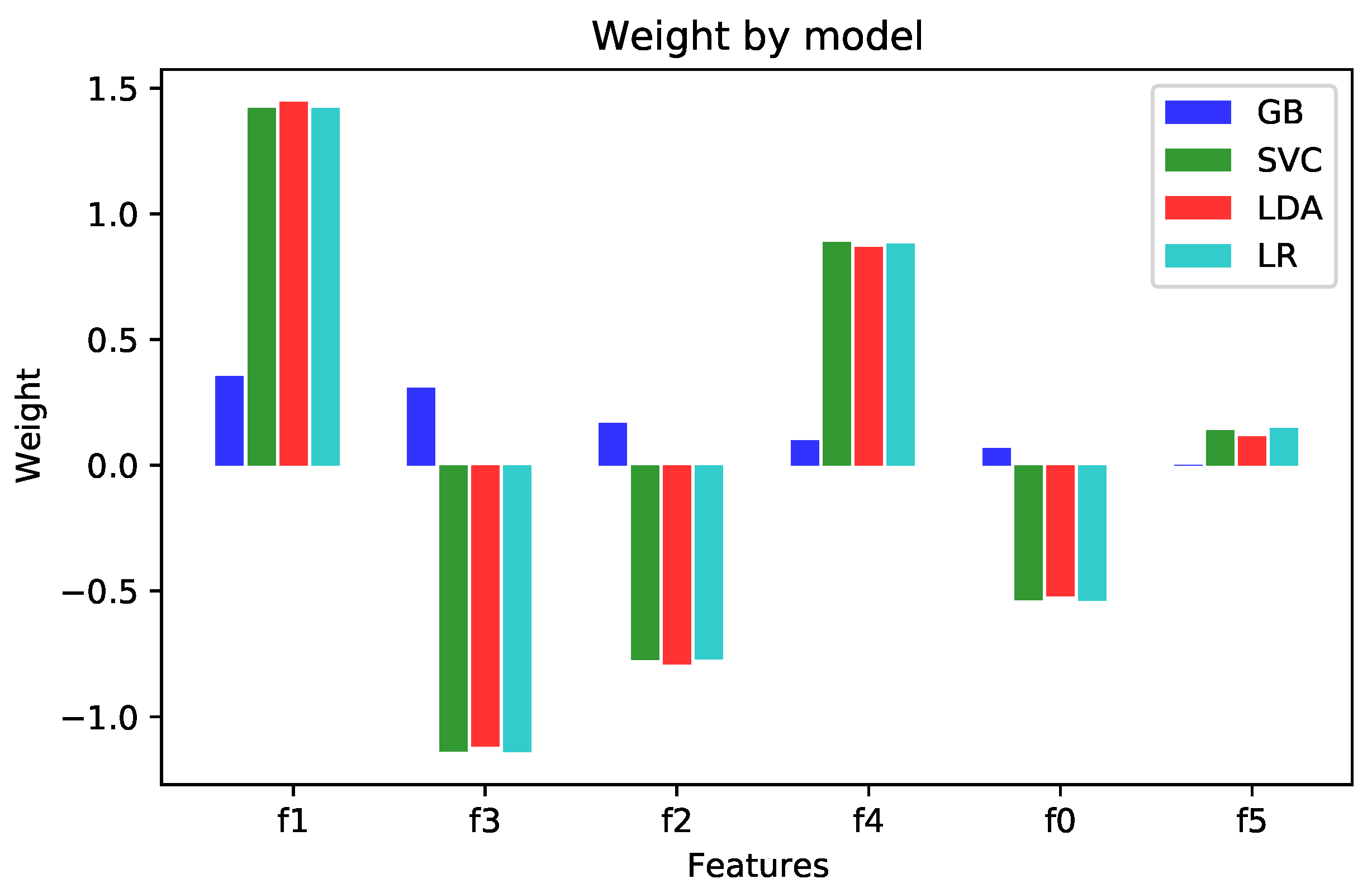
A third experiment aimed to measure the contribution of each of the variables to the final model. Figure 5, collects the weights for the MIFF analysis, and can be understood as the contributions of the different experiments. Additionally, as can be appreciated in the figure, although all features presented similar weights, f 3 and f 1 received slightly higher weights than the others. An exception to this was found for f 5 , which had a small weight in all ML algorithms we analyzed. This result is consistent with the fact that this feature was effectively irrelevant and misclassified by the algorithm, thereby allowing further adjustment to the model.

4.3. German Credit Dataset

In this experiment, we applied the knowledge previously acquired in the synthetic dataset, but this time using actual data from the German credit dataset. The main purpose of this was to verify if the results obtained with real data would be the same, when using the same methodology as for the synthetic dataset.
Following the previously scrutinized methodology, our FS technique was applied to this new dataset. Results for the German credit dataset with the IVI technique and all the ML algorithms are presented in Figure 6. A number of features were unfailingly identified as relevant for all the ML algorithm, following the same pattern observed with the synthetic dataset and showing consistency with previously described results in terms of these repeated informative features. Equivalently to prior descriptive analysis, features were classified as RFF if they had been selected in all the ML algorithms used, and MIFF if they had been selected by at least in two of them.
Four experiments were guided using one hundred epochs of bootstrap tests in order to evaluate the statistical significance. Results in Table 2 show systematically an almost insignificant standard deviation, with independence from the dataset. The method–characteristic paired models show high accuracy in all cases: the values were close to 75% in all cases. Regarding the methods, they all showed similar values for the different sets of variables, except the SVC method, which presented a drop of 4% with respect to the rest for the set of RFF variables. Singularly, this same method (SVC) offered the best result with the remaining feature set, by systematically surpassing the rest of the methods and reaching a maximum of 76.63% with the MIFF filter. On the other hand, lower results were steadily found, although still strong, with the GB method. Accuracy was worse by more than 1% for the feature sets at best, with the sole exception of the RFF, with which SVC presented a decline even larger. From a feature-set perspective, the results were very homogeneous among the methods, and singularly better in the case of MIFF, due to precision figures over 75.10% in all cases. On the contrary, the RFF filter showed not only uneven behavior across methods, but also consistently poorer results. The results shown here correlate highly with those of the analysis carried out with the synthetic dataset, thereby validating the hypotheses formulated during the exercise.
All the ML algorithms using MIFF showed higher accuracy using the IVI features. The only exception was LR, which had a slight reduction in accuracy. Those results are consistent with those previously obtained, and again, FS using MIFF improved the training procedure in terms of computational efficiency, by reducing the number of features needed to reach higher accuracy, and thus confirming empirically the hypothesis settled with the synthetic dataset.
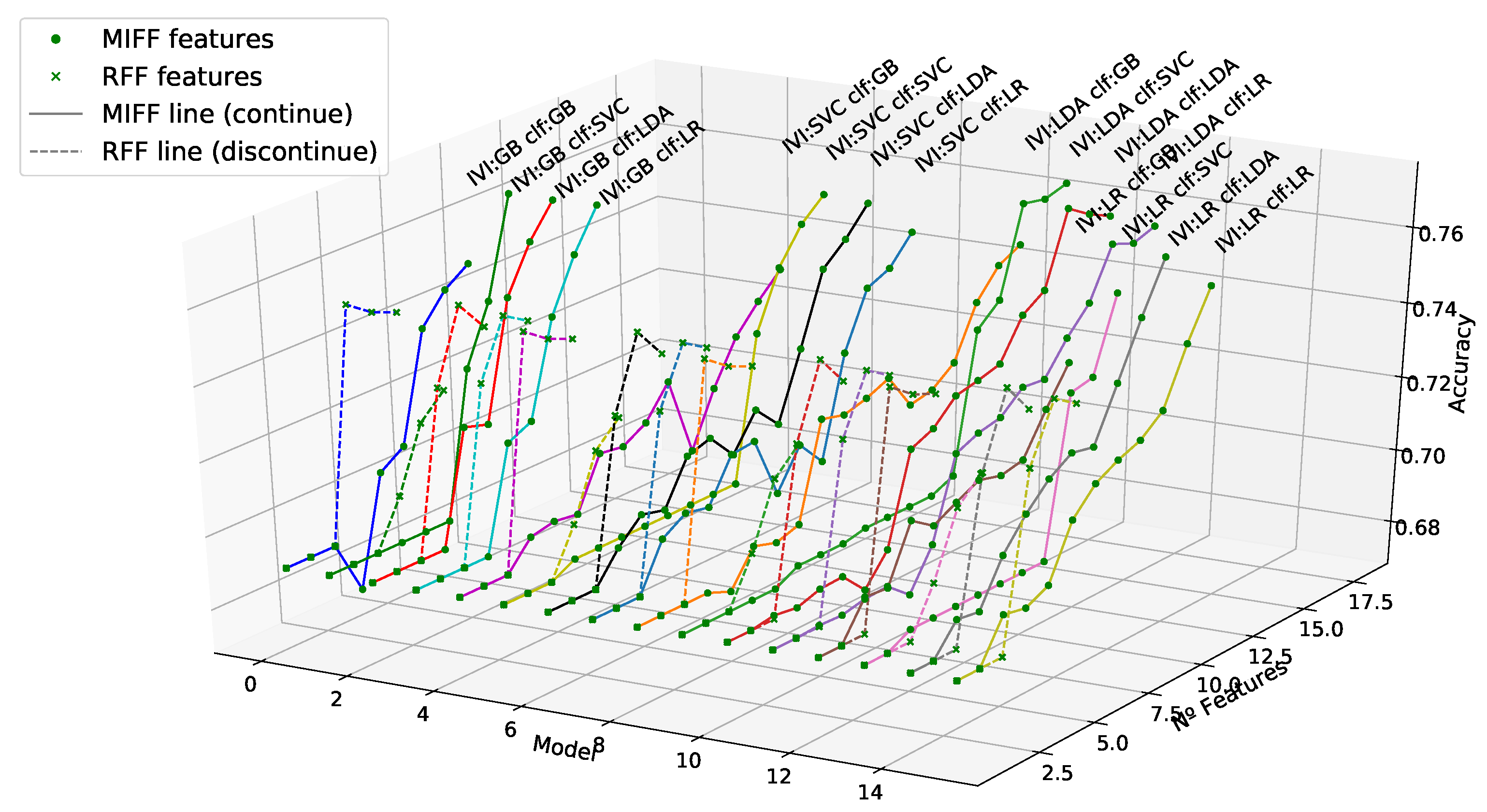
Equivalent representations appeared earlier for all evaluated models and available features. They are depicted in Figure 7 and Figure 8. In particular, in Figure 7 we see the parallel and comparative processes followed in the IVI algorithm and the RFF filtered features; and in Figure 8, we also see the corresponding analysis for MIFF. It can be observed in figure that accuracy systematically increased in all cases when relevant features were added toward the maximum value. After that, the accuracy remained stable, despite the redundant and noisy features being added. Furthermore, when MIFF and RFF filters were used, we reduced the number of features to reach the maximum accuracy against the standard IVI approach. The best results were obtained using the MIFF filter. Figure 7 show slightly lower accuracy when compared to IVI. As we mentioned earlier, this is related to the extremely restricted set of candidates allowed to become relevant features when using this filtering technique.
In the informative representation in Figure 8a,b, we can see an interesting effect. Using RFF, we had an explosive increment in terms of accuracy, while using a relatively small set of features, but we did not achieve the maximum. However, when using MIFF, an initial slight ramp-up was obtained, but we achieved the maximum in accuracy, surpassing IVI’s accuracy while using a smaller number of features. This situation was the same in all models, as represented in Figure 9 from a different perspective. In this representation, for the reader’s convenience, the high dimensionality of the data is restricted in terms of the number of features to just the relevant ones, in an attempt to visualize this effect across the different plots.
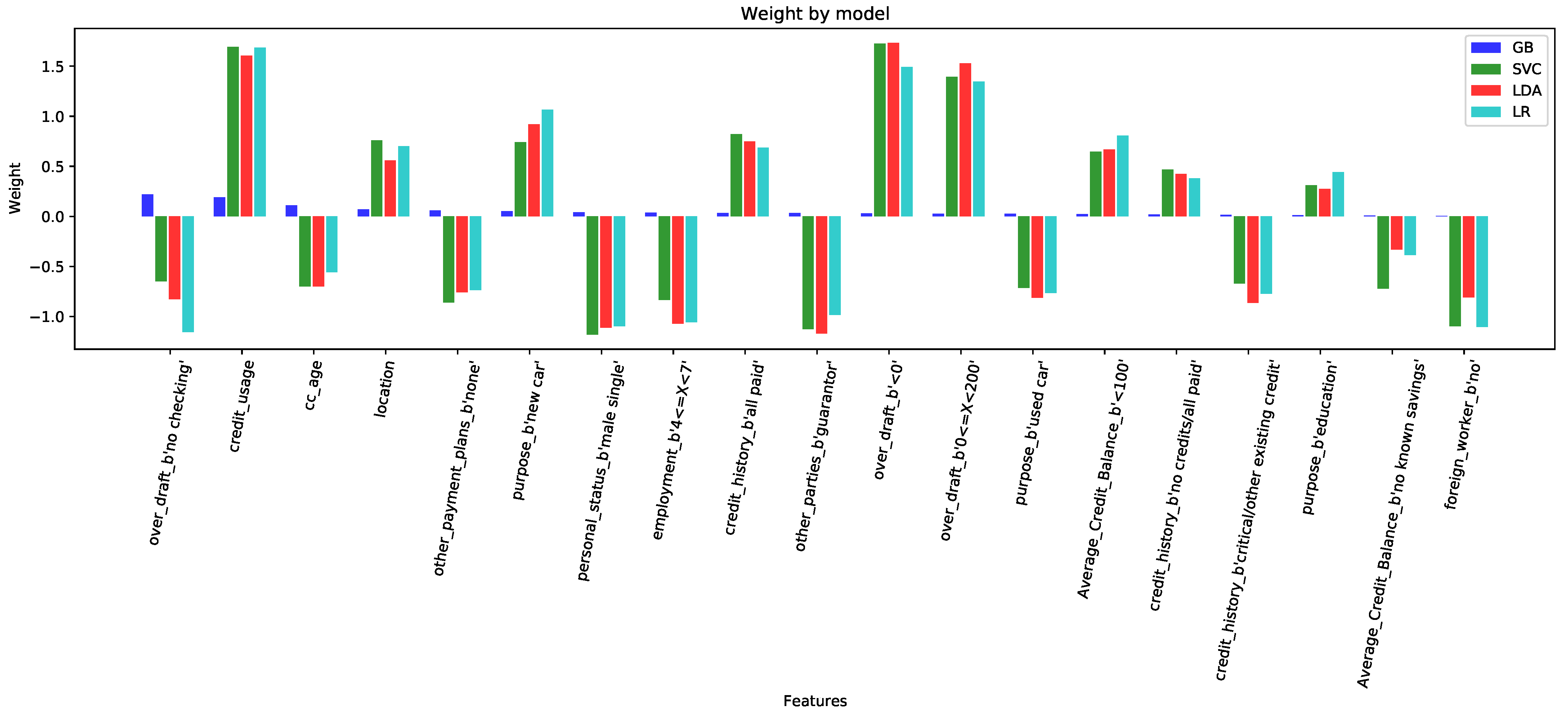
In the same way as it previously analyzed in the synthetic dataset, the contributions to the decision process of the weights of the features in all the experiments were evaluated. Again, (i) the smaller contributions or weights of a number of variables meant they were classified as noisy or redundant, (ii) the large contributions of other variables classified them as relevant, and (iii) a number of them had small to medium contributions and were redundant, but were misclassified. Figure 10 illustrates the coefficients corresponding to the MIFF features. The representation illustrates the existence of large-contribution variables, over ±1.0 (over_draft_<0, credit_usage, purpose_new_car, employment, other_parties_guarantor), and the large-contribution ones over ±0.5 (credit_history_other_existing_credits, average_credit_balance_<100, location purpose_ education), and a small proportion of variables with a significantly lower contribution less than 0.5 (purpose_rent, current_balance, credit_history_no_credits, foreign_worker). This last group very likely corresponds to the redundant variables that were incorrectly classified, and therefore, subjected to be excluded at a later stage. It is necessary to point out at this point the identification of 3 variables outstanding the general classification with contributions 50% higher than their peers. In particular, credit_usage was the most relevant feature for all algorithms, and the second most relevant was over_draft_<0. These results are consistent with literature [36,37] and with the companion paper [12]. This special subset should be conveniently analyzed separately from an interpretability perspective, given this remarkable behavior: it is not only more important than the rest, but was consistently reproduced in every method. We should mentioned here the special situation of the GB method. Although significance apparently offered proportional matching with the rest of the methods, its magnitudes are far lower than those of the rest of the methods, following its behavior in the synthetic scenario.

5. Discussion and Conclusions

In this paper, we elaborated on the possibility of applying the almost ubiquitous current ML techniques to CFD. One of the main drawbacks of these technologies is that even though they are extremely effective and powerful in almost all disciplines, they are mostly black boxes: it is virtually impossible to decode the way the variables are treated internally. This last statement is intrinsically incompatible with regulations issued by administrative bodies, as whatever tool is used should be compliant with non-discriminatory rules and transparency. In this work, we proposed a novel methodology to address the mentioned drawbacks when applying ML to the CFD problem, which uses state-of-the-art algorithms capable of quantifying the information of the variables and their relationships. This approach offers a new method for interpretability to cope with this multifaceted dilemma. In this paper, we presented an intensive analysis of a number of statistical learning techniques (GB, SVR, LR, and LDA), together with new feature selection procedures, applied both on a synthetic dataset for development, and on a real dataset for validation. As a general conclusion of all the experiments, we can say that it is possible to develop an ML model supporting the novel feature selection techniques presented in this paper. The result will not only provide the detection of CFD, but also at the same time allows one to visualize the contribution of each feature in the decision process, thereby offering the necessary interpretability of the model and the results. To deal with the complex dichotomy of machine learning tools and interpretability, we elaborated on informative features and calculated their contributions to the decision process, leaving aside black boxes and minimizing potential biases by using state-of-the-art ML techniques. We claim that it is possible to build robust, explanatory linear models that simultaneously meet the regulatory constraints and use the power of ML techniques. To do so, our work was twofold. First, we developed a synthetic dataset to define and fine-tune the models. Second, the successful models were later on applied to a real dataset to verify generalization and consistency.
The main conclusions when analyzing the synthetic dataset are described hereafter. First, using the IVI model, we were able to systematically identify the features with informative value. Additionally, the use of a subset of the variables when applying the filters described in this paper improved the performance in terms of the computational efficiency by limiting the number of variables. We found that all noisy and redundant variables were consistently excluded from this extended method. Two different filtering procedures were proposed, RFF and MIFF. The first one is much more restrictive and was the fastest way to reach a reasonable level of accuracy, but failed in the classification of a number of features. On the other hand, the second filter, although it had redundant variables, did not misclassify any noisy features. As the interpretations of linear models were proposed based on the final weights obtained, and considering that far lower contributions were found for these redundant features, the joint application of MIFF and weight evaluation could be considered as an efficient and accurate model, even in the cases when redundant features are identified. Based on these results, we conclude that formulation and classification using IVI, together with RFF and MIFF filtering, offers an automatic and efficient system that improves the generalization and prediction capabilities of CFD on synthetic datasets.
The results of applying these methodologies to the German Credit dataset [5,38] were in general terms consistent with the previous findings on the synthetic dataset. The results obtained suggested that the use of presented method not only improved the results (with a 4% accuracy increase compared to previous papers’ results) but also enhances computational efficiency by reducing the number of features. From a methodological perspective, the applied model was confirmed to be valid, as accuracies for all method–characteristic models were homogeneous. Their lowerest values were close to 75% on average with a standard deviation of close to 2%. From a computational perspective, and considering the four different sub-sets of features evaluated, namely, all features, IVI features, MIFF, and RFF, the last two offered significant reductions in the number of variables, thereby significantly improving the computer’s workload. For both, accuracy was high, although MIFF offered higher stability in the results across methods. Detailed analysis showed that RFF managed to incorporate effectively none but relevant variables, but missed in certain cases some of the relevant ones. MIFF managed in all cases to include them all, but also included some redundant ones. The integration of redundant variables in MIFF did not generate any lack of accuracy or stability in the predictive capacity, and they could be removed at a later stage, as their contributions (weights) steadily had far lower magnitudes compared to their peers’ weights. On the contrary, in the RFF case, the rapid convergence due to the adjusted base of variables selected in this subset was not accompanied by the most stable behavior in the results, due to the absence of some significant variables due to the incorrect classification. Thus, there was an up to four percent reduction in precision compared to other the models. We can therefore argue at this point, that a very strict strategy in the search for truly informative variables, such as RFF, although it intensively accelerates convergence and computational efficiency, sometimes prevents all informative variables from being collected, causing a lack of convergence or instability in the results. On the other hand, not so aggressive strategies for selecting variables, such as the MIFF, offer greater flexibility, which, although they sometimes allow the selection of redundant variables, maximize the probability of incorporating all the relevant ones, without excessively increasing the computational needs. For this reason, the use of IVI classification techniques, together with the application of MIFF selection sets, can offer the right balance between computational requirements and accuracy. From an ML perspective, the methodology used is consistent due to all the methods showing similar results with little differences for each of the feature sets, although SVR again was the method that provided the best results, and GB under-performed slightly among its peers.
Finally, as introduced earlier, the system presented here, using exclusively linear strategies, offers a powerful interpretable state-of-the-art technique beating the predictability of other more sophisticated and more difficult to interpret ML applications. This approach paves the way for greater interpretability, as the contributions of the different final features could be matched to the weights of those very same variables. Following the synthetic analysis, coefficients of the variables tended to be very high for relevant features, and low or very low for redundant or noisy features, respectively. For the specific case of MIFF, there were some very highly contributing variables and highly contributing ones, plus a small proportion of variables with significantly lower contributions, which happened to be redundant. Three variables stood out with contributions 50% higher than their peers. This special subset of variables should be specially evaluated as a key and supporting features of the model, as they not only showed large contributions, but consistently reproduced the modulating power in every implemented method. It should be noted now that these variables (average credit with unknown savings, clients with overdraft, and purpose of credit being for a new car) were already identified in the literature [36,37], conveying, therefore, double validation: of the results and of the model itself.
As a general conclusion, we can state that it is possible to create in five steps, an unbiased, interpretable classification model: (i) an initial IVI analysis; (ii) benchmarking of ML classifiers to reduce the bias; (iii) FS and filtering of the variables; (iv) a bootstrap analysis for statistical significance estimations; (v) a feature significance calculation, based on the coefficients, which pave the way toward the desired interpretability of the ultimate model. This model offers a novel multi-tapper approach for effective, efficient, and interpretable classification that can be used in many fields, but specifically where black boxes are not acceptable due to regulatory restrictions. Hence, the innovative techniques presented in this work in relation to the FS applying the aforementioned relevance filters through cross-analysis of different classification techniques, have proven to be not only more effective than previous techniques, but offer more computationally efficient methods for the analysis. With all that, we reduced the potential biases and opened the way to develop models for legally restricted applications.
The necessary interpretability for models to be used in CFD could be obtained through the analysis of the coefficient for each of the variables for every single classification. These coefficients, already limited in number after this strict process of validation, constitute the contributions of all of these variables to the decisions or recommendations obtained. We can discuss at this point not only the importance of these coefficients to estimating said contributions, but also using them as a second validation tool for the variables, having observed that the variables that participate with less intensity could be eliminated without relevant effects from a practical point of view. Additionally, this same combination of factors can be jointly interpreted as an analysis pattern offering a direct characterization of the finally implemented model.
Further analyses could be eventually proposed based on our concepts, e.g., to provide deep learning anomaly detection strategies. In the companion paper [12], we present a thoughtful analysis of non-linear models in that direction, leveraging the valid results and conclusions of the present work.
We can conclude that the proposed methodology, in combination with state-of-the-art linear ML models, can provide fast methods to discover the most relevant features in CFD problems. The black-box methods can be left behind, and we can instead generate interpretable models in which the potential biases are minimized. With this work, the groundwork has been laid to provide interpretability to CFD, and we shall see how this will affect the legal and ethical considerations.

Author Contributions

J.C.-U. and S.M.-R. (Santiago Moral-Rubio and Sergio Muñoz-Romero) conceptualized the problem, elaborated the state-of-the-art. J.C.-U., F.-J.G.-B. and J.-L.R.-Á. elaborated the methods and methodology, and conducted the experiments and developed the discussion and conclusions. All authors discussed the results and contributed to write the final manuscript. All authors have read and agreed to the published version of the manuscript.

Funding

This work is partly supported by research grants, meHeart RisBi (PID2019-104356RB-C42), miHeart-DaBa (PID2019-104356RB-C43), and BigTheory (PID2019-106623RB-C41), from Agencia Estatal de Investigación of Science and Innovation Ministry; and cofunded by FEDER funding. It is also partially supported by REACT EU grants from the Community of Madrid and Rey Juan Carlos University funded by the Next Generation EU.

Institutional Review Board Statement

Not applicable.

Informed Consent Statement

Not applicable.

Data Availability Statement

The data that support the findings of this study are openly available in the different repositories as described in references.

Conflicts of Interest

The authors declare no conflict of interest. All co-authors agree with the contents of the manuscript and declare that there is no financial interest in the present paper.

References

  1. Dornadula, V.; Geetha, S. Credit Card Fraud Detection using Machine Learning Algorithms. Procedia Comput. Sci. 2019, 165, 631–641. [Google Scholar] [CrossRef]
  2. Buchanan, B.G. Artificial Intelligence in Finance; Zenodo: London, UK, 2019. [Google Scholar]
  3. Brause, R.; Langsdorf, T.; Hepp, M. Neural data mining for credit card fraud detection. In Proceedings of the 11th International Conference on Tools with Artificial Intelligence, Chicago, IL, USA, 9–11 November 1999; pp. 103–106. [Google Scholar]
  4. Chen, C.; Lin, K.; Rudin, C.; Shaposhnik, Y.; Wang, S.; Wang, T. An Interpretable Model with Globally Consistent Explanations for Credit Risk. arXiv 2018, arXiv:1811.12615. [Google Scholar]
  5. Pumsirirat, A.; Yan, L. Credit Card Fraud Detection using Deep Learning based on Auto-Encoder and Restricted Boltzmann Machine. Int. J. Adv. Comput. Sci. Appl. 2018, 9, 18–25. [Google Scholar] [CrossRef]
  6. Ana, F. Artificial Intelligence in Financial Services; Banco de España: Madrid, Spain, 2019. [Google Scholar]
  7. Machine Learning in UK Financial Services; Bank of England: London, UK, 2019.
  8. Yan, H.; Lin, S. New Trend in Fintech: Research on Artificial Intelligence Model Interpretability in Financial Fields. Open J. Appl. Sci. 2019, 09, 761–773. [Google Scholar] [CrossRef] [Green Version]
  9. Wall, L. Some Financial Regulatory Implications of Artificial Intelligence. J. Econ. Bus. 2018, 100, 55–63. [Google Scholar] [CrossRef]
  10. Wedge, R.; Kanter, J.M.; Veeramachaneni, K.; Rubio, S.M.; Perez, S.I. Solving the False Positives Problem in Fraud Prediction Using Automated Feature Engineering. In Machine Learning and Knowledge Discovery in Databases; Brefeld, U., Curry, E., Daly, E., MacNamee, B., Marascu, A., Pinelli, F., Berlingerio, M., Hurley, N., Eds.; Springer International Publishing: Cham, Switzerland, 2019; pp. 372–388. [Google Scholar]
  11. Carvalho, D.; Pereira, E.; Cardoso, J. Machine Learning Interpretability: A Survey on Methods and Metrics. Electronics 2019, 8, 832. [Google Scholar] [CrossRef] [Green Version]
  12. Chaquet-Ulldemolins, J.; Gimeno-Blanes, J.; Moral-Rubio, S.; Rojo-Álvarez, J.L. On the Black-box Challenge for Fraud Detection using Machine Learning (II): Non-Linear Analysis through Interpretable Autoencoders. submitted to this issue. submitted to this issue.
  13. Muñoz-Romero, S.; Gorostiaga, A.; Soguero-Ruiz, C.; Mora-Jiménez, I.; Rojo-Álvarez, J.L. Informative variable identifier: Expanding interpretability in feature selection. Pattern Recognit. 2020, 98, 107077. [Google Scholar] [CrossRef]
  14. Ribeiro, M.; Singh, S.; Guestrin, C. Why Should I Trust You?: Explaining the Predictions of Any Classifier. In Proceedings of the Conference of the North American Chapter of the Association for Computational Linguistics: Demonstrations, San Francisco, CA, USA, 13–17 August 2016; pp. 97–101. [Google Scholar]
  15. Bertsimas, D.; Delarue, A.; Jaillet, P.; Martin, S. The Price of Interpretability. arXiv 2019, arXiv:1907.03419. [Google Scholar]
  16. Petrasic, K.; Saul, B.; Greig, J.; Bornfreund, M.; Lamberth, K. Algorithms and Bias: What Lenders Need to Know; White & Case LLP: New York, NY, USA, 2017. [Google Scholar]
  17. Lipton, Z. The Mythos of Model Interpretability. Commun. Assoc. Comput. Mach. 2016, 61. [Google Scholar]
  18. Bellman, R. Adaptive Control Processes: A Guided Tour. (A RAND Corporation Research Study); Princeton University Press: Princeton, NJ, USA, 1961; Volume XVI, pp. 255–260. [Google Scholar]
  19. Chen, L. Curse of Dimensionality; Springer US: Boston, MA, USA, 2009. [Google Scholar]
  20. Bachu, V.; Anuradha, J. A Review of Feature Selection and Its Methods. Cybern. Inf. Technol. 2019, 19, 3. [Google Scholar]
  21. Yu, L.; Liu, H. Efficient Feature Selection via Analysis of Relevance and Redundancy. J. Mach. Learn. Res. 2004, 5, 1205–1224. [Google Scholar]
  22. Torkkola, K. Feature Extraction by Non Parametric Mutual Information Maximization. J. Mach. Learn. Res. 2003, 3, 1415–1438. [Google Scholar]
  23. Ibrahim, N.; Hamid, H.; Rahman, S.; Fong, S. Feature selection methods: Case of filter and wrapper approaches for maximising classification accuracy. Pertanika J. Sci. Technol. 2018, 26, 329–340. [Google Scholar]
  24. Kohavi, R.; John, G.H. Wrappers for feature subset selection. Artif. Intell. 1997, 97, 273–324. [Google Scholar] [CrossRef] [Green Version]
  25. Chen, X.; Jeong, J.C. Enhanced recursive feature elimination. In Proceedings of the Sixth International Conference on Machine Learning and Applications, Cincinnati, OH, USA, 13–15 December 2007; pp. 429–435. [Google Scholar]
  26. Kaya Uyanık, G.; Güler, N. A Study on Multiple Linear Regression Analysis. Procedia-Soc. Behav. Sci. 2013, 106, 234–240. [Google Scholar] [CrossRef] [Green Version]
  27. Witten, D.M.; Tibshirani, R. Penalized classification using Fisher’s linear discriminant. J. R. Stat. Soc. Ser. B (Stat. Methodol.) 2011, 73, 753–772. [Google Scholar] [CrossRef] [Green Version]
  28. Vapnik, V.N. Statistical Learning Theory; Wiley-Interscience: Hoboken, NJ, USA, 1998. [Google Scholar]
  29. Schlkopf, B.; Smola, A.J.; Bach, F. Learning with Kernels: Support Vector Machines, Regularization, Optimization, and Beyond; The MIT Press: Cambridge, MA, USA, 2018. [Google Scholar]
  30. Zhang, Y. Support Vector Machine Classification Algorithm and Its Application. In International Conference on Information Computing and Applications; Springer: Berlin/Heidelberg, Germany, 2012; pp. 179–186. [Google Scholar]
  31. Rojo-Álvarez, J.L.; Martínez-Ramón, M.; Munoz-Marí, J.; Camps-Valls, G. Digital Signal Processing with Kernel Methods, 1st ed.; Wiley-IEEE Press: Hoboken, NJ, USA, 2018. [Google Scholar]
  32. Natekin, A.; Knoll, A. Gradient Boosting Machines, A Tutorial. Front. Neurorobot. 2013, 7, 21. [Google Scholar] [CrossRef] [Green Version]
  33. Bentéjac, C.; Csörgő, A.; Martínez-Muñoz, G. A comparative analysis of gradient boosting algorithms. Artif. Intell. Rev. 2020, 54, 1937–1967. [Google Scholar] [CrossRef]
  34. Friedman, J.H. Stochastic gradient boosting. Comput. Stat. Data Anal. 2002, 38, 367–378. [Google Scholar] [CrossRef]
  35. Dua, D.; Graff, C. UCI Machine Learning Repository; UCI: Irvine, CA, USA, 2017. [Google Scholar]
  36. Macailao, M. Raising the Red Flags: The Concept and Indicators of Occupational Fraud. J. Crit. Rev. 2020, 7, 26–29. [Google Scholar]
  37. DiNapoli, T.P.; State of New York Office of the State Comptroller. Red Flags for Fraud. State N. Y. Off. State Comptrol. 2018, 1–14. Available online: https://apipa2010.pitiviti.org/files/fraud_redflats.pdf (accessed on 27 February 2022).
  38. Gonzalez, J.; Holder, L.; Cook, D. Graph Based Concept Learning. FLAIRS Conf. 2000. Available online: https://www.aaai.org/Papers/FLAIRS/2001/FLAIRS01-073.pdf (accessed on 27 February 2022).
Figure 1. Methodology. In the FS, the features are transformed into a coefficient space using IVI with different ML algorithms (CME, GB, SVC, LDA, and LR). Through the use of confidence intervals and relations between feature, we compose the rankings of informative features. In the filter step, we apply the filters to detect recurrent features and maximally-informative features. Finally, in the last step, using the features provided by the filter we trained, with linear models, we get the weights assigned to each of these features. Those weights reflect the importance of features in the decision process.
Applsci 12 03328 g001
Figure 2. Results of the IVI algorithm for each ML technique on the synthetic dataset. In rows are the different ML techniques: covariance multiplication estimator (CME), support vector machine classification (SVC), gradient boosting (GB), linear regression (LR), and linear discriminant analysis (LDA). In columns are the different features, as defined previously. Green stands for scenarios where features were identified as relevant. Red stands for features not identified as relevant during the analysis.
Applsci 12 03328 g002
Figure 3. Graphical results for accuracy through of incorporation of the features in sequential order of relevance to RFF models, enabling us see the evolution in accuracy as each feature is added. In 3D plots (a), we can see number of features on the x-axis, on the y-axis are the different ML algorithms (GB, SVC, LDA, and LR), and the accuracy is on the z-axis. For each ML algorithm, we present the evolution of features selected in IVI as a continuous line and the features selected by the filter as a dashed line. In (b), we show a comparison between filters and IVI. For clarity and simplicity, we only show one comparative sample. In (b), the red line represents a dummy classifier that makes predictions with the most frequent class, and the green dashed line shows the results of the classifier trained with all features.
Applsci 12 03328 g003
Figure 4. Graphical results for accuracy through of incorporation of the features in sequential order of relevance to MIFF models, enabling us see the evolution in accuracy as each feature is added. In 3D plots (a), we can see number of features on the x-axis, on the y-axis are the different ML algorithms (GB, SVC, LDA, and LR), and the accuracy is on the z-axis. For each ML algorithm, we present the evolution of features selected in IVI as a continuous line and the features selected by the filter as a dashed line. In (b), show a comparison between filters and IVI. For clarity and simplicity, we only show one comparative sample. In (b), the red line represents a dummy classifier that makes predictions with the most frequent class, and the green dashed line shows the results of the classifier trained with all features.
Applsci 12 03328 g004
Figure 5. Features’ weights. Graphical weights for the features selected by the MIFF filter. Each color bar represents a different ML technique: GB, SVC, LDA, LR.
Applsci 12 03328 g005
Figure 6. Results of the IVI algorithm for each ML technique on the real dataset. In rows are the different ML techniques: CME, SVC, GB, LR, and LDA. In columns have the different features. Green stands for scenarios where features were identified as relevant. Red means a feature was not identified as relevant during the analysis.
Applsci 12 03328 g006
Figure 7. Graphical results for accuracy through of incorporation of the features in sequential order of relevance to RFF models, enabling us see the evolution in accuracy for every feature that is added. In 3D plots (a), we can see number of features on the x-axis, on the y-axis are the different ML algorithms (GB, SVC, LDA, and LR), and the accuracy is on the z-axis. For each ML algorithm, we present the evolution of features selected in IVI as a continuous line and the features selected by the filter as a dashed line. In (b), show a comparative between filters and IVI. For clarity and simplicity we only show one comparative sample. In (b), red line represents a dummy classifier that makes predictions with the most frequent class, and the green line dashed is the results of the classifier trained with all features.
Applsci 12 03328 g007
Figure 8. Graphical results for accuracy through of incorporation of features in sequential order of the relevance for MIFF models, enabling us see the evolution in accuracy for every feature that is added. In 3D plots (a), we can see number of features on the x-axis, on the y-axis are the different ML algorithms (GB, SVC, LDA, and LR), and the accuracy is on the z-axis. For each ML algorithm, we present the evolution of features selected in IVI as a continuous line and the features selected by the filter as a dashed line. In (b), we show a comparatison between filters and IVI. For clarity and simplicity, we only show one comparative sample. In (b), the red line represents a dummy classifier that makes predictions with the most frequent class, and the green dashed line represents the results of the classifier trained with all features.
Applsci 12 03328 g008
Figure 9. Graphical results for accuracy through incorporation of the relevant features in sequential order for RFF and MIFF. We can see number of features in the x-axis. Along the y-axis are the different ML algorithms (GB, SVC, LDA, and LR). The accuracy is along the z-axis. For each ML algorithm, we present the evolution of features selected by the MIFF filter as a continuous line and the features selected by the RFF filter as a dashed line.
Applsci 12 03328 g009
Figure 10. Features’ weights. Graphical weights for the features selected in MIFF filter. Each color bar represents a different ML technique: GB, SVC, LDA, LR.
Applsci 12 03328 g010
Table 1. Statistical results for accuracy of the ML methods in synthetic dataset. Mean and standard deviation of the results for one-hundred-resample analysis. In rows are the results for the different ML methods. In columns are the different set of features included in the analysis. Columns from left to right, represent all available features, IVI-relevant features, MIFF features, and RFF features.
method_ClassifierAcc_all_featuresIVI (Relevant)Acc_fs_MIFFAcc_fs_RFF
GB 0.9393 ± 0.005034 0.9319 ± 0.004903 0.9393 ± 0.005209 0.8961 ± 0.005413
SVC 0.9870 ± 0.003195 0.9705 ± 0.003803 0.9872 ± 0.002951 0.9062 ± 0.005112
LDA 0.9787 ± 0.003127 0.9709 ± 0.003638 0.9877 ± 0.003356 0.9063 ± 0.004634
LR 0.9865 ± 0.002669 0.9711 ± 0.003586 0.9881 ± 0.003579 0.9062 ± 0.004958
Table 2. Statistical results for accuracy for different ML methods on the real dataset. Means and standard deviations of the results for one-hundred-resample analysis.
method_ClassifierAcc_all_featuresIVI (Relevant)Acc_fs_MIFFAcc_fs_RFF
GB 0.7433 ± 0.0171 0.7431 ± 0.01911 0.7510 ± 0.0191 0.7446 ± 0.0190
SVC 0.7580 ± 0.0170 0.7598 ± 0.0205 0.7663 ± 0.0204 0.7256 ± 0.0228
LDA 0.7533 ± 0.0172 0.7463 ± 0.0203 0.7573 ± 0.0193 0.7443 ± 0.0213
LR 0.7563 ± 0.0174 0.7576 ± 0.0190 0.7563 ± 0.0189 0.7476 ± 0.0209
Publisher’s Note: MDPI stays neutral with regard to jurisdictional claims in published maps and institutional affiliations.

