Feature Mining: A Novel Training Strategy for Convolutional Neural Network

Abstract

In this paper, we propose a novel training strategy named Feature Mining for convolutional neural networks (CNNs) that aims to strengthen the network’s learning of the local features. Through experiments, we found that different parts of the feature contain different semantics, while the network will inevitably lose a large amount of local information during feedforward propagation. In order to enhance the learning of the local features, Feature Mining divides the complete feature into two complementary parts and reuses this divided feature to make the network capture different local information; we call the two steps Feature Segmentation and Feature Reusing. Feature Mining is a parameter-free method with a plug-and-play nature and can be applied to any CNN model. Extensive experiments demonstrated the wide applicability, versatility, and compatibility of our method.

1. Introduction

Convolution neural networks (CNNs) have made significant progress on various computer vision tasks, e.g., image classification [1,2,3,4], object detection [5,6,7], and segmentation [8,9]. However, the large scale and tremendous parameters of CNNs may result in overfitting and reduce generalization, which brings great challenges to network training. A series of training strategies have been proposed to solve these problems, including data augmentation [10,11,12], batch normalization [13], and knowledge distillation [14]. Those approaches aim to improve the performance and generalization of CNNs by changing the input, feature space, or output.

In particular, some methods improve the generalization by strengthening the learning of the feature. As a representative regularization method, Dropout [15] randomly discards parts of the internal features in the network to improve the influence of the remaining features. SpatialDropout [16] randomly discards all the channels rather than individual activations for the CNN. DropBlock [17] randomly drops some contiguous regions of a feature map. Besides, self-distillation distills the knowledge itself to improve the utilization of internal features. Be your own teacher (BYOT) [18] improves the efficiency of network training by squeezing the knowledge in the deeper portion of the networks into the shallow ones. As a state-of-the-art self-distillation method, classwise self-knowledge distillation [19] improves the generalization of the same kind of images from the perspective of intra-class distillation. In this paper, we focused on developing a new training strategy for CNNs to strengthen the network’s learning of the local features. Different from the above methods, which enhance the local feature learning by discarding parts of the feature or using a distillation technique, our method divides the complete feature into two complementary parts and reuses this divided feature to make the network capture different local information, which is able to achieve better generalization with negligible extra computation cost.

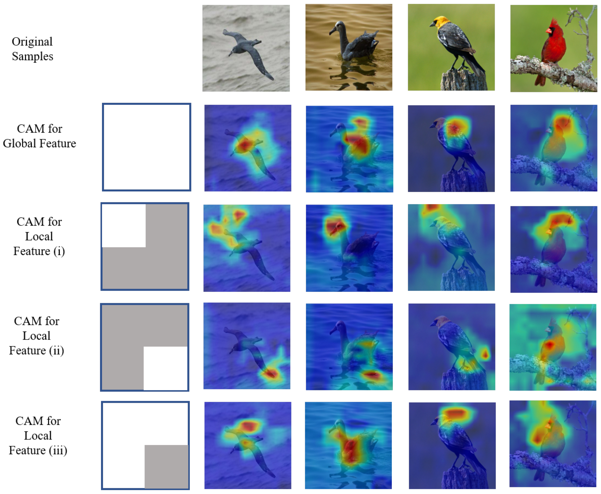
Our motivation stems from a phenomenon in the training process of CNNs: information loss inevitably occurs after going through the pooling layer, which may lead to the CNN’s inadequate learning of the local features. We performed several visualization experiments [20] to explore the difference between the global features and the local features. The result empirically suggested that different parts of the feature contain different semantics, and the local features contain different semantics compared with the global features. However, the network will inevitably lose the local information during feedforward propagation. Making the network contain more local feature knowledge is a benefit to the training, but how to make the local features of images sufficiently mined by the network is a great challenge.

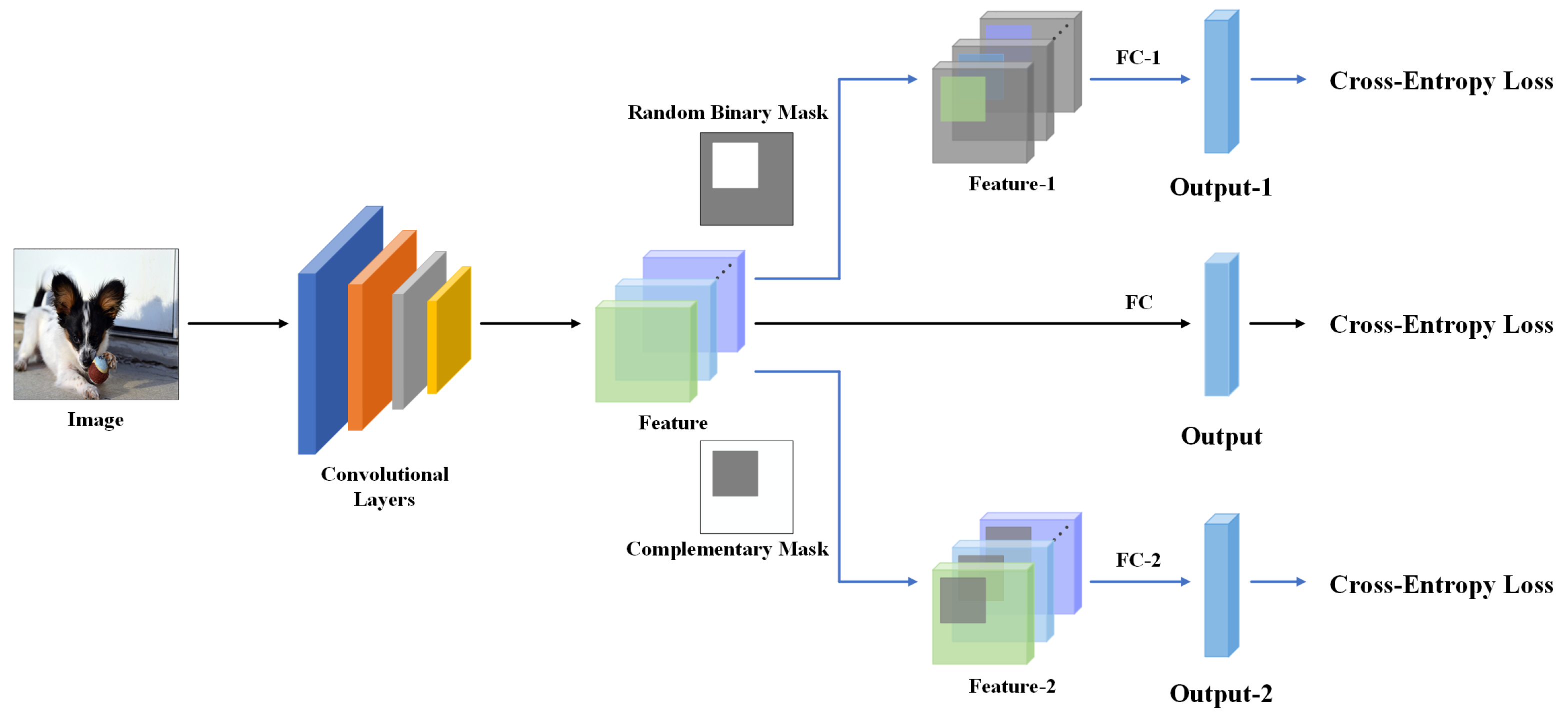
Based on the above observations, we propose a parameter-free training method: Feature Mining, which aims to make the network efficiently learn the local features. This strategy requires two steps: Feature Segmentation and Feature Reusing. During Feature Segmentation, we divide the feature into two complementary parts by two binary masks. Feature Reusing denotes that these two parts of the feature will respectively pass through a global average pooling layer and a fully connected layer to generate two independent outputs, and the three cross-entropies will be added to form the final loss function. In this way, different local features can jointly participate in the network training with the global features, so that the network is able to learn more abundant feature expressions. Feature Mining can also be extended to any layer of the CNN. Specifically, adding Feature Mining in the last two layers of the network not only further improves the performance of the network, but also strengthens the shallow layers’ learning ability. Due to its inherent simplicity, Feature Mining has a plug-and-play nature. Besides, we do not need to set any hyperparameters for Feature Mining, which can reduce the operating cost and maintain the stability of our method for performance improvement.

We demonstrate the effectiveness of our simple, yet effective training method with different network structures, such as ResNet [4], DenseNet [21], Wide ResNet [22], and PyramidNet [23], for image classification tasks on various datasets including CIFAR100 [24], TinyImageNet, and ImageNet [2]. A great accuracy boost was obtained by Feature Mining, higher than the Dropout [15,16,17] and self-distillation methods [18,19]. In addition, our training method has strong compatibility and can be superimposed on the mainstream data augmentation [12] and self-distillation methods. Besides, we verified the wide applicability of Feature Mining in fine-grained classification [25], object detection [26], and practical scenarios [27,28].

In summary, we made the following principle contributions in this paper:

• We propose a novel training strategy, Feature Mining, which aims to make the network learn the local features more efficiently. Our method enjoys a plug-and-play nature and is parameter-free;
• The proposed training approach can obviously improve the network’s performance with little extra training cost and can be superimposed on the mainstream training methods;
• Experiments for four kinds of CNN architectures on three kinds of datasets were conducted to prove the generalization of this technique. The performance in different scenarios demonstrated the wide applicability of our method.

2. Related Works

Methods for reducing information loss in CNNs: The pooling layer decreases the size of the activation maps to reduce the computational requirements of the CNN, which would inevitably incur information loss. Many strategies try to alleviate this problem by reforming the structure of the pooling layer. Random shifting [29] embeds random shifting in the downsampling layers during the training process to generate more robust features in the network. S3Pool [30] replaces the regular downsampling by a more general stochastic version and can be seen as performing implicit data augmentation by introducing distortions in the feature maps. Inspired by the human visual system, detail-preserving pooling [31] magnifies spatial changes and preserves important structural detail to make the CNN focus on local spatial changes. Based on softmax normalization, SoftPool [32] preserves the descriptive activation features, while remaining computationally and memory efficient. Note that although our approach also attempts to reduce information loss and strengthen local feature learning as the above methods, we did not change the structure of the pooling layer, but reused the segmented features for efficient learning.

Dropout methods: The Dropout methods aim to improve the generalization of neural networks. Dropout [15] injects noise into the feature space by randomly zeroing the activation function to avoid overfitting. SpatialDropout [16] randomly discards all the channels rather than individual activations to improve the generalization of the CNN. DropBlock [17] randomly drops some contiguous regions of a feature map for better network performance. Besides, References [33,34,35,36] also proposed variants of Dropout. These Dropout methods enhance local feature learning by discarding other parts of the feature, but Feature Mining divides the feature into different parts and reuses all of them.

Data augmentation methods: Data augmentation is an effective strategy for network training. Random cropping and horizontal flipping [1] are the most commonly used data augmentation techniques. By randomly removing contiguous sections of the input images, Cutout [10] improves the robustness of the network. Random erasing [11] randomly selects a rectangle region in an image and erases its pixels with random values. Input Mixup [12] creates virtual training examples by linearly interpolating two input data and the corresponding one-hot labels. Inspired by Cutout and Mixup, CutMix [37] cuts patches and pastes them among the training images. Feature Mining is complementary to the above data augmentation methods such as Mixup because it operates on the feature level without changing the data processing.

Self-distillation methods: Knowledge distillation [14] is proposed for model compression. Unlike traditional knowledge distillation methods that require teacher and student models, self-distillation distills knowledge itself. Data distortion [38] transfers knowledge between different augmented versions of the same training data. Be your own teacher [18] improves the efficiency of network training by squeezing the knowledge in the deeper portion of the networks into the shallow ones. Classwise self-knowledge distillation [19] improves the generalization of the same kind of images from the perspective of intra-class distillation. Both self-distillation and Feature Mining could improve the utilization of the internal features. Experiments showed that our method outperformed existing self-distillation methods and can be superimposed on self-distillation.

3. Materials and Methods

3.1. Observation

In order to explore the semantic difference among the local features, we conducted an experiment on the visualization of the CNN. During the network training, we multiplied the feature of the last layer of the network by different fixed binary masks, so that only part of the feature in the last layer of the network could participate in the network training. We used class activation maps (CAMs) [20] to visualize the trained model. Specifically, ResNet-50 [23] trained on CUB-200-2011 [25] was chosen as the baseline model. All the models were trained from scratch for 200 epochs with a batch size of 32, and the learning rate was decayed by a factor of 0.1 at Epochs 100 and 150. The choice of epochs and batch size followed the common practice. Training with a few epochs cannot guarantee network convergence, while training with too many epochs may lead to the overfitting of the network. Network convergence can be guaranteed without overfitting when training with 200 epochs. Theoretically, the larger the batch size, the better the network performance is. However, a large batch size will result in a large memory overhead. When the batch size was set to 32, we could obtain the best network performance under existing computing resources.

As shown in Figure 1, the second line shows the visualization results of the global features in the last layer, while the following lines show the visualization results of different local features. We can see that the complete features generally focused on the global information of the target, while the local features focused more on the relevant local information according to their locations. Obviously, the image information concerned in the local features is different from that of the global features, and the semantic information between different local features is different. However, the network only obtains the output depending on the global feature information due to the feedforward mechanism of the CNN, which may cause the loss of information contained in the local features. How can we make full use of the local features in the network training? We see how to address this issue next.

3.2. Feature Mining

Feature Mining is designed to improve the learning of the local features by the CNN. Here, we present some notations that will be used in the following. Formally, for a given training sample $(x,y)$, $x\in {\mathbb{R}}^{W\times H\times C}$ denotes the training image and $y\in Y=\{1,2,3,...,C\}$ denotes the training label. For a network with N classifiers, we use X to represent the network’s internal features and $a^n$ to represent the output of the nth branch. Next, we describe the proposed Feature Mining strategy in detail, which consists of two steps, i.e., Feature Segmentation and Feature Reusing, as depicted in Figure 2.

3.2.1. Feature Segmentation

In order to make the network learn different local features, we first divided the high-dimensional feature into two complementary parts by using a binary mask. In the training phase, the training sample $(x,y)$ would be processed by the network, and we could obtain the feature X of this sample. After obtaining the complete feature $X_0$ before the last pooling layer, we generate a binary mask M with a bounding box with coordinates $B=(r_x,r_y,r_w,r_h)$ indicating the cropping regions on the binary mask. As CutMix [37], the box coordinates are uniformly sampled according to:

$$\begin{array}{cc}\hfill & r_x\sim \mathrm{Unif}(0,W),r_w=W\sqrt{1-\lambda }\hfill \\ \hfill & r_y\sim \mathrm{Unif}(0,H),r_h=H\sqrt{1-\lambda }\hfill \end{array}$$

(1)

making the cropped area ratio $\frac{r_w{r}_h}{WH}=1-\lambda$. $\lambda$ is sampled from the uniform distribution $(0,1)$. The elements in B are set to one, and other elements in M are set to zero. We define the segmentation operation as:

$$\begin{array}{cc}\hfill X_1& =X_0\odot M\hfill \\ \hfill X_2& =X_0\odot (1-M)\hfill \end{array}$$

(2)

where $X_1$ and $X_2$ are complementary parts of $X_0$ and contain different local semantics of $X_0$, which means $X_1$ only contains the feature information within B while $X_2$ only contains the feature information outside B. We used the block to segment the feature based on the characteristics of the CNN: adjacent neurons have similar semantics, and the block-form segmentation can ensure that the two parts of the feature have great differences, which could make the network efficiently obtain different local features. Note that this operation can also be applied to any layer to obtain different representative features and is not limited by the network structure. For a detailed discussion of the effect of the segmentation method, please refer to Section 4.5. Besides, many methods preprocess the data to improve the Feature Segmentation. However, our approach only performs segmentation on the feature space and is based on raw data.

3.2.2. Feature Reusing

After Feature Segmentation, we obtain a set of extra complementary features $X_1$ and $X_2$ from the complete feature $X_0$. Based on the observation in Section 3.1, the semantics of $X_0$, $X_1$, and $X_2$ are different from each other. In order to make the network learn the information of these three parts of the knowledge simultaneously, we added two groups of global average pooling layers and fully connected layers as two new branches based on the original network. $X_1$ and $X_2$ will respectively enter their own global average pooling layer and fully connected layer to obtain the new outputs $a^1$ and $a^2$, and the output of the complete feature $X_0$ is $a^0$. We used softmax to compute the predicted probability of the nth output for class i:

$$\begin{array}{cc}\hfill & p_i^n=\frac{exp\left(a_i^n\right)}{{\sum }_{j=1}^{C}exp\left(a_j^n\right)}\hfill \end{array}$$

(3)

where C denotes the number of ground-truth labels. The probabilities $p^1$ and $p^2$ correspond to these two outputs and will also be calculated with the real label of the image to obtain the new cross-entropies. We added these cross-entropies to the cross-entropy of $X_0$ to obtain the final loss function. To sum up, the loss function of the whole neural network consists of the cross-entropy of each branch, which can be written as:

$$\begin{array}{c}\hfill loss=\sum _{i=0}^{n}CrossEntropy(p^i,y)\end{array}$$

(4)

where n denotes the number of branches including the main branch and two new branches and y denotes the ground-truth label. These independent cross-entropies work together on the backpropagation of the network and affect the gradient update of the network parameters to make the neural network learn the knowledge information of the whole feature and the local features simultaneously, so as to achieve the purpose of Feature Reusing.

3.2.3. Application

Feature Mining can be theoretically plugged behind any convolutional layer within a CNN and can be superimposed on multiple layers at once during training. In practice, we chose the last one or two layers for our method. Note that the binary masks used for the segmentation were generated randomly in each network iteration, which makes the network continuously learn the different complementary parts of the feature so that the training of the whole network is more efficient and robust. We stress again that, as a lightweight parameter-free strategy, Feature Mining was added to these networks only in the training phase, and the network in the test phase was unchanged.

4. Results and Discussion

In this section, we investigate the effectiveness of Feature Mining for multiple computer vision tasks. We first conducted extensive experiments on image classification (Section 4.1) and fine-grained image classification (Section 4.2). Next, we studied the effect of Feature Mining on object detection (Section 4.3). Besides, we evaluated the performance of our method in practical scenarios (Section 4.4). We also show the ablation study of Feature Mining in Section 4.5. All experiments were performed with Pytorch [39] on Tesla M40 GPUs. The highest validation accuracy over the full training course was chosen as the result. If not specified, all results reported were averaged over four runs. Note that all the accuracy results are pixel based.

4.1. Image Classification

4.1.1. CIFAR Classification

The CIFAR100 dataset [24] consists of 60,000 32 × 32 color images of 100 classes, each with 600 images including 500 training images and 100 test images. For ResNet [4] and Wide ResNet [22], the mini-batch size was set to 128, and the models were trained for 300 epochs with an initial learning rate of 0.1 decayed by a factor of 0.1 at Epochs 150 and 225. We changed the batch size to 64 when training with DenseNet [21]. As mentioned in [23], we changed the initial learning rate to 0.5 and decreased it by a factor of 0.1 at Epochs 150 and 225 when training PyramidNet [23].

Comparison with the Dropout methods: We adopt ResNet-56, ResNet-110, ResNet-164, DenseNet-100-12, Wide ResNet-28-10, and PyramidNet-110-270 as the baselines to evaluate Feature Mining’s generalization for different layers and structures of networks. We tested Feature Mining with the last layer and the last two layers. Dropblock [17] was applied to the output of the first two groups. Dropout [15] and SpatialDropout [16] were applied to the output of the penultimate group.

Table 1. Validation accuracy (%) on the CIFAR100 dataset using the CNN architectures of ResNet-56, ResNet-110, ResNet-164, DenseNet-100, WRN-28-10, and PyramidNet-110-270 (top accuracy in bold). FM denotes Feature Mining. The p-value is the statistical comparison between FM (2 layers) and the best-performing Dropout method within the independent-samples t test.

Method	ResNet-56	ResNet-110	ResNet-164	DenseNet-100	WRN-28-10	PyramidNet-110
Baseline	73.71 ± 0.28	74.71 ± 0.23	74.98 ± 0.23	77.25 ± 0.20	79.35 ± 0.20	81.54 ± 0.31
Dropout	73.81 ± 0.27	74.69 ± 0.33	75.15 ± 0.11	77.45 ± 0.12	79.21 ± 0.15	81.31 ± 0.24
SpatialDropout	74.38 ± 0.17	74.76 ± 0.12	75.34 ± 0.09	77.97 ± 0.16	79.63 ± 0.09	81.60 ± 0.17
DropBlock	73.92 ± 0.10	74.92 ± 0.07	75.51 ± 0.14	77.33 ± 0.09	79.44 ± 0.24	81.57 ± 0.21
FM (1 layer)	74.55 ± 0.11	75.79 ± 0.08	76.51 ± 0.13	78.24 ± 0.12	79.75 ± 0.16	82.13 ± 0.25
FM (2 layers)	75.35 ± 0.07	76.90 ± 0.13	78.31 ± 0.21	78.78 ± 0.09	80.90 ± 0.22	82.87 ± 0.15
p-Value	0.018003	0.000634	0.000193	0.039	0.00495	0.01008

shows that Feature Mining outperformed other baselines consistently. In particular, Feature Mining improved the top-1 accuracy of the cross-entropy loss from 74.98% to 78.31% (independent-samples t test, p-value = 0.000177 < 0.001) of ResNet-164 under the CIFAR100 dataset.

Our method, only used in the last layer, was better than the performance of the three Dropout methods, and we considered the reason to be that Dropout and its variants strengthen the part of the neurons’ learning by discarding other parts of the neurons, which may cause information loss during the training phase. Feature Mining can make the network simultaneously learn the different regions of the feature without information loss, so that the network can achieve better performance. We can also find that the network performance of Feature Mining used in the last two layers was much better than that only used in the last layer, which indicates that the local feature in the front layer is also beneficial to the network training.

Comparison with self-distillation methods: We also compared our method with self-distillation techniques such as be your own teacher (BYOT) [18] and classwise knowledge distillation (CS-KD) [19]. BYOT improved the performance of the network by making the shallow network learn the knowledge of the last layer. Therefore, we took the output of the last layer in ResNet-110 as the teachers of all the front layers and provided the final results after ensembling for a fair comparison. Besides, CS-KD improved the generalization of the same kind of images from the perspective of intra-class distillation. Note that we only chose ResNet-110 as the baseline model due to the limitation of computing resources, but it can be seen from the results in Table 1 that the improvement of our method in a deeper network (ResNet-110) was more obvious than that in a shallow network (ResNet-164). Therefore, the performance of our method on ResNet-110 was able to prove its advantage because of its generalization.

As shown in

Table 2. The performance comparison with self-distillation methods on the CIFAR100 dataset.

Method	Validation Accuracy (%)
ResNet-110	74.71 ± 0.23
ResNet-110+BYOT	76.68 ± 0.14
ResNet-110+CS-KD	75.92 ± 0.08
ResNet-110+FM	76.90 ± 0.21
ResNet-110+FM+BYOT	77.34 ± 0.16
ResNet-110+FM+CS-KD	77.68 ± 0.11

, Feature Mining showed better top-1 accuracy on ResNet-110 compared with BYOT and CS-KD. Note that BYOT added extra overhead in the training, while the time of our method was negligible. Besides, we combined Feature Mining with these two methods and improved the top-1 accuracy of ResNet-110 from 76.68% to 77.34% (independent-samples t test, p-value = 0.046 < 0.05) of BYOT and from 75.92% to 77.68% (independent-samples t test, p-value = 0.000322 < 0.001) of CS-KD. This shows that Feature Mining does not conflict with these methods; even in the case of improving the performance of the front layer (BYOT) or reducing the gap within the class (CS-KD), the performance can still be improved by strengthening the learning of the local features.

Comparison with the data augmentation method: We investigated orthogonal usage with other types of regularization methods such as Mixup [12]. Mixup utilizes convex combinations of input pairs and corresponding label pairs for training. We combined our method with Mixup regularization by combining the input and label processed by Mixup with ResNet-110, which uses Feature Mining on the last two layers.

Table 3. The performance comparison with Mixup on the CIFAR100 dataset.

Method	Validation Accuracy (%)
ResNet-110	74.71 ± 0.23
ResNet-110+Mixup	77.78 ± 0.25
ResNet-110+FM	76.90 ± 0.12
ResNet-110+FM+Mixup	79.13 ± 0.17
ResNet-164	74.98 ± 0.23
ResNet-164+Mixup	79.22 ± 0.12
ResNet-164+FM	78.31 ± 0.09
ResNet-164+FM+Mixup	81.04 ± 0.20

shows the effectiveness of our method combined with Mixup regularization. Interestingly, this simple idea significantly improved the performance of the classification task. In particular, our method improved the top-1 accuracy of Mixup regularization from 79.22% to 81.04% (independent-samples t test, p-value = 0.001 < 0.01) on ResNet-164, which proves our method is also compatible with the data augmentation method.

4.1.2. Tiny ImageNet Classification

The Tiny ImageNet dataset is a subset of the ImageNet [2] dataset with 200 classes. Each class has 500 training images, 50 validation images, and 50 test images. All images have a 64 × 64 resolution. The test set label is not publicly available, so we used the validation set as a test set for all the experiments on Tiny ImageNet following the common practice. The results are summarized in

Table 4. The performance comparison on the Tiny ImageNet dataset. The best accuracy is achieved by Feature Mining.

Method	Validation Accuracy (%)
ResNet110	62.42 ± 0.25
ResNet110+Dropout	62.32 ± 0.05
ResNet110+Spatial Dropout	62.55 ± 0.10
ResNet110+DropBlock	63.13 ± 0.29
ResNet110+BYOT	63.03 ± 0.17
ResNet110+CS-KD	64.29 ± 0.11
ResNet110+FM	65.22 ± 0.06

. Feature Mining achieved the best performance 65.22% on Tiny ImageNet compared with the Dropout methods, BYOT and CS-KD, +2.80% (independent-samples t test, p-value = 0.000062 < 0.001) higher than the baseline. This proves that our method is also generalized for datasets with different data sizes. These results also show that Feature Mining has wide applicability and performs better than other regularization or self-distillation methods on different datasets.

4.1.3. ImageNet Classification

ImageNet-1K [2] contains 1.2M training images and 50K validation images labeled with 1K categories. To verify the scalability of our method, we evaluated our method on the ImageNet dataset with ResNet-50, which is the commonly used model for ImageNet with high performance and acceptable computing overhead. The model was trained from scratch for 300 epochs with a batch size of 256, and the learning rate was decayed by a factor of 0.1 at Epochs 75, 150, and 225. As reported in

Table 5. The performance comparison on the ImageNet dataset on ResNet-50.

Method	Validation Accuracy (%)
ResNet-50	76.32 ± 0.02
ResNet-50+FM	77.26 ± 0.04

, our method improved by 0.94% (independent-samples t test, p-value = 0.001 < 0.01) the top-1 accuracy compared with the baseline. This shows that our training strategy is also effective for image recognition in large-scale datasets.

4.2. Fine-Grained Image Classification

Fine-grained image classification aims to recognize similar subcategories of objects under the same basic level category. The difference of fine-grained recognition compared with general category recognition is that fine-grained subcategories often share the same parts and usually can only be distinguished by the subtle differences in the texture and color properties of these parts. 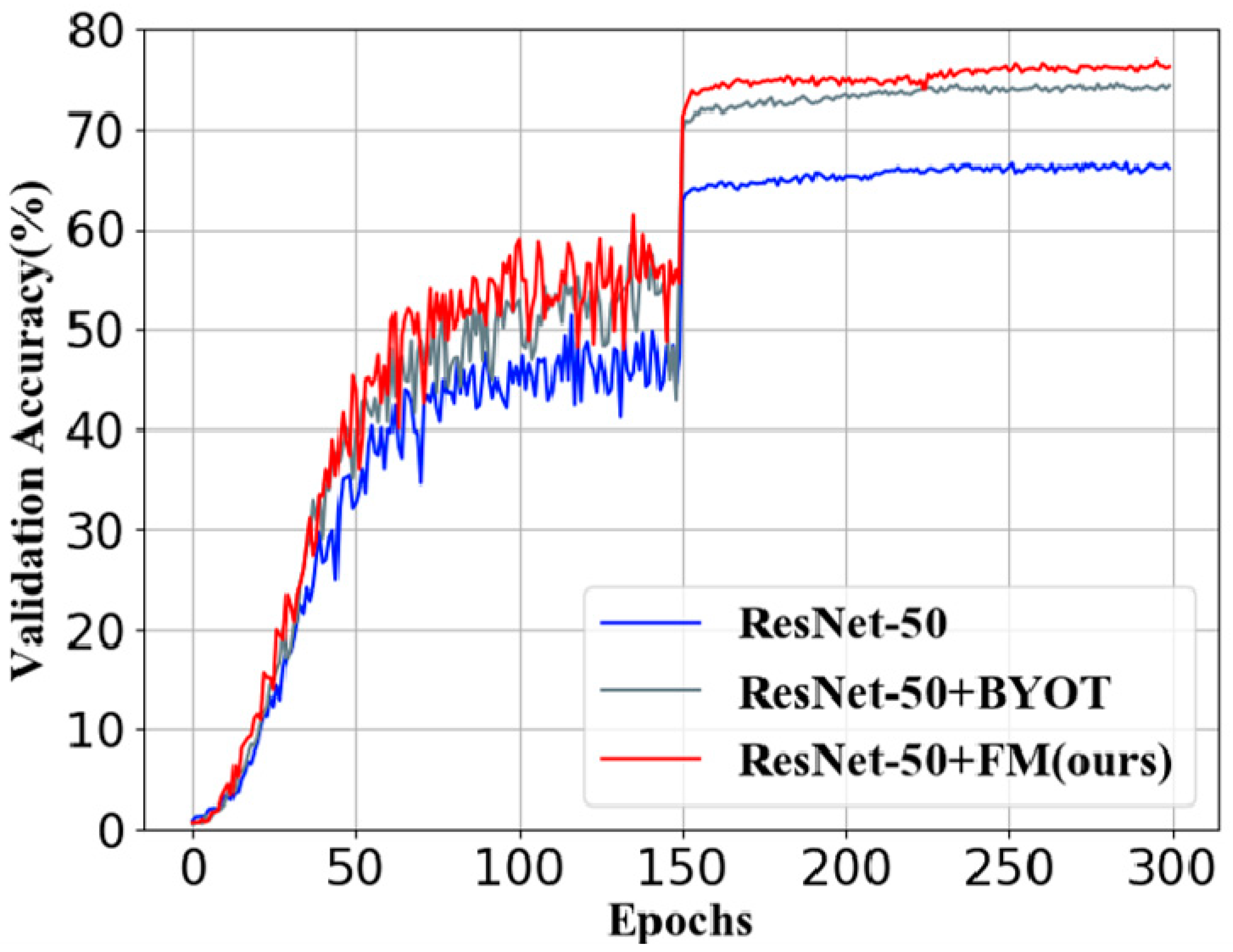CUB-200-2011 [25] is a widely used fine-grained dataset that consists of images of 200 bird species. There are about 30 images for training for each class. We used ResNet-50 to test the performance of our method on CUB-200-2011 to verify the generalization of different types of computer vision tasks. For a fair comparison, the model was trained from scratch for 300 epochs with a batch size of 32, and the learning rate was decayed by a factor of 0.1 at Epochs 150 and 225.

As shown in

Table 6. The performance comparison with self-distillation methods on the CUB-200-2011 dataset.

Method	Validation Accuracy (%)
ResNet-50	66.73 ± 0.34
ResNet-50+BYOT	74.60 ± 0.41
ResNet-50+CS-KD	74.81 ± 0.23
ResNet-50+FM	76.26 ± 0.27

, we improved the accuracy of ResNet-50 from 66.73% to 76.26% (independent-samples t test, p-value = $2.8532\times {10}^{-7}$ < 0.001), +9.53% with Feature Mining, which significantly surpassed previous self-distillation methods. It also shows that fully utilizing feature information has a high gain effect even on fine-grained image classification, which requires more subtle differences. Figure 3 shows the validation accuracy comparison among the baseline, BYOT, and Feature Mining on CUB-200-2011 with ResNet-50. The accuracy of BYOT and our method was much higher than the baseline, and the accuracy of Feature Mining was higher than that of BYOT.

4.3. Object Detection

In this subsection, we show that Feature Mining can also be applied for training the object detector on the Pascal VOC dataset [26]. The RetinaNet [40] framework was chosen as the baseline model, which is composed of a backbone network and two task-specific subnetworks. The ResNet-50 backbone was initialized with the ImageNet-pretrained model and then fine-tuned on Pascal VOC 2007 and 2012 trainval data. The models were evaluated on the VOC 2007 test data using the mAP metric. We followed the fine-tuning strategy of the original method.

As shown in

Table 7. The performance comparison on the Pascal VOC dataset.

Method	Validation Accuracy (%)
RetinaNet	70.14 ± 0.17
RetinaNet+FM pre-trained	71.11 ± 0.14

, the ResNet-50 pre-trained with Feature Mining achieved a better accuracy (71.11%), +0.97% (independent-samples t test, p-value = 0.013 < 0.05) higher than the baseline performance. The result suggests that the model trained with Feature Mining is also an effective training approach for object detection.

4.4. Practical Scenarios

A. Label noise problem: In practical scenarios, the dataset is full of error labels because of the expensive and time-consuming labeling process, which could seriously affect the performance of the model. This phenomenon is known as the label noise problem. We set up experiments with noisy datasets to see how well Feature Mining performed for different types and amounts of label noise.

Following [27,41], we corrupted these datasets manually on CIFAR-100. Two types of noisy labels were considered: (1) symmetry flipping: each label was set to an incorrect value uniformly with a certain probability; (2) pair flipping: labelers may only make mistakes within very similar classes. We use $ϵ$ to denote the noise rate.

Table 8. Average test accuracy on noisy CIFAR-100 using ResNet-110 with and without Feature Mining.

Noise Type	$\mathit{ϵ}$	Method	Accuracy (%)
Symmetric Flip	0.5	ResNet-110	45.73
		ResNet-110+FM	53.31 (+7.58)
	0.2	ResNet-110	61.16
		ResNet-110+FM	68.12 (+6.96)
Pair Flip	0.5	ResNet-110	35.73
		ResNet-110+FM	38.78 (+3.05)
	0.2	ResNet-110	63.83
		ResNet-110+FM	71.22 (+7.39)

compares the results with and without Feature Mining using ResNet-110. Our method made huge improvements on different types and amounts of noise compared with the baseline (which only uses cross-entropy to classify). One possible implication of the improvement is that our method can make the convolutional layers’ training more sufficient, and the robust network has stronger anti-noise ability. Together, these results provide strong proofs that Feature Mining helps raise the internal noise tolerance of the network.

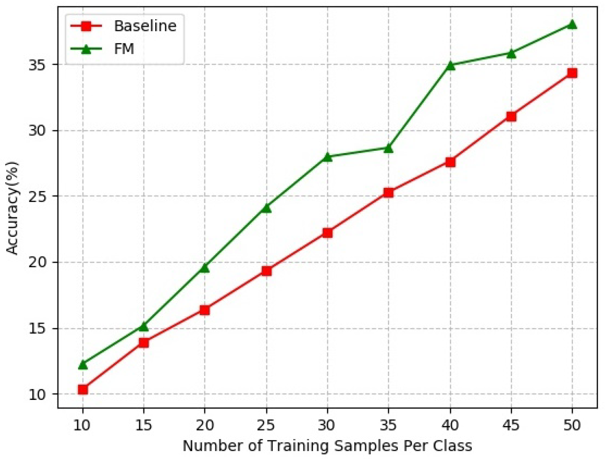
B. Small sample size problem: In some real industrial scenarios, the size of the dataset may be small, which would bring difficulty to the network training. Besides, Reference [42] mentioned that reducing the size of the training dataset can measure the generalization performance of the models. Therefore, we evaluated the effectiveness of Feature Mining on the small sample size problem along with varying the size of the training data. Due to the limitation of the computing resources, we chose ResNet-56 as the baseline model.

We constructed a series of sub-datasets of CIFAR-100 via randomly choosing samples for each class. Figure 4 compares the results obtained from ResNet-56 trained with and without our strategy. Feature Mining was used on the last two layers of the network. From the graph, we can see that our method yielded much higher accuracies compared to the vanilla setting on all of the sub-datasets, in accordance with the expectations. The performance of Feature Mining proves that our method can effectively improve the generalization of CNNs.

4.5. Ablation Study

A. Influence of different choices of Feature Mining on network performance: We explored different design choices for Feature Mining, and these choices were classified into two groups.

As shown in

Table 9. Performance of Feature Mining variants on ResNet-56.

Method	Accuracy (%)
ResNet-56	73.71 ± 0.28
ResNet-56+FM (1 layer)	74.55 ± 0.11
ResNet-56+FM (2 layers)	75.35 ± 0.07
ResNet-56+FM (3 layers)	75.29 ± 0.12
ResNet-56+Dropout-FM	74.12 ± 0.23
ResNet-56+SpatialDropout-FM	74.01 ± 0.17
ResNet-56+non-complementary FM	74.23 ± 0.09

, the first group discusses the number of layers using Feature Mining. ResNet-56 contains three layers, and we tested the Feature Mining on the last layers, the last two layers, and all three layers. All three models outperformed the baseline model from 74.55% to 75.35%, while the model with the last two layers using Feature Mining performed better than others. This shows that the penultimate layer’s local feature is beneficial to the network training. While the feature of the first layer does not contain mature semantics, adding learning of the feature in the first layer is not beneficial for the network training.

The second group focuses on the Feature Segmentation approach. The Feature Segmentation determines the additional feature pattern of the network learning, which plays a crucial role in the performance of our method. Dropout-FM denotes that the binary mask is set by random points as the Dropout. SpatialDropout-FM denotes that the feature is divided by channels as the SpatialDropout. The performance of these segmentation approaches could not compete with Feature Mining, which proves the segmentation feature based on the block region can ensure a larger difference between the two parts and make the network learn more feature information. Non-complementary FM denotes that we randomly chose two parts of the feature instead of the complementary ones; its performance was still not as good as the complementary way, which again verifies that the difference between the two parts of the feature is important.

B. Analysis of time and memory overhead:

Table 10. Computation cost introduced by Feature Mining. The statistics were obtained on a Tesla M40 GPU with a batch size of 128. The training time is averaged over the first 300 iterations.

Method	GPU Memory (MB)	Training Time (s/iter)
ResNet-56	1740	0.094
ResNet-56+FM (1 layer)	1773	0.098
ResNet-56+FM (2 layers)	1959	0.113

provides some complexity statistics of Feature Mining, which shows that the computation cost introduced by Feature Mining is negligible, especially when our method is only used in the last layer. Besides, this additional cost is introduced only in the training phase, and the inference cost is not increased.

5. Conclusions

In this paper, we proposed a novel training strategy named Feature Mining that aims to strengthen a CNN’s learning of the local features. Feature Mining divides the complete feature into two complementary parts and reuses the divided feature to make the network capture different local information for efficient training. Our method has a plug-and-play nature and can be applied to any CNN model. Extensive experiments proved that Feature Mining brought stable improvement to different classification datasets on various models and could be applied to various tasks, including fine-grained image classification, object detection, label noise, and the small data regime. On CIFAR-100 classification, applying Feature Mining to ResNet-164 brought +3.33% top-1 accuracy improvement. On CUB-200-2011, fine-grained image classification, applying Feature Mining to ResNet-50, significantly improved the performance of the baseline by +9.53%. Besides, Feature Mining is complementary to data augmentation and self-distillation methods. For future work, we plan to find better segmentation strategies for Feature Mining by using reinforcement learning.

References

1. Krizhevsky, A.; Sutskever, I.; Hinton, G.E. Imagenet classification with deep convolutional neural networks. Adv. Neural Inf. Process. Syst. 2012, 25, 1097–1105. [Google Scholar] [CrossRef]
2. Russakovsky, O.; Deng, J.; Su, H.; Krause, J.; Satheesh, S.; Ma, S.; Huang, Z.; Karpathy, A.; Khosla, A.; Bernstein, M.; et al. Imagenet large scale visual recognition challenge. Int. J. Comput. Vis. 2015, 115, 211–252. [Google Scholar] [CrossRef] [Green Version]
3. Szegedy, C.; Liu, W.; Jia, Y.; Sermanet, P.; Reed, S.; Anguelov, D.; Erhan, D.; Vanhoucke, V.; Rabinovich, A. Going deeper with convolutions. In Proceedings of the IEEE Conference on Computer Vision and Pattern Recognition, Boston, MA, USA, 7–12 June 2015; pp. 1–9. [Google Scholar]
4. He, K.; Zhang, X.; Ren, S.; Sun, J. Deep residual learning for image recognition. In Proceedings of the IEEE Conference on Computer Vision and Pattern Recognition, Las Vegas, NV, USA, 27–30 June 2016; pp. 770–778. [Google Scholar]
5. Girshick, R. Fast r-cnn. In Proceedings of the IEEE International Conference on Computer Vision, Santiago, Chile, 7–13 December 2015; pp. 1440–1448. [Google Scholar]
6. Ren, S.; He, K.; Girshick, R.; Sun, J. Faster r-cnn: Towards real-time object detection with region proposal networks. Adv. Neural Inf. Process. Syst. 2015, 28, 91–99. [Google Scholar] [CrossRef] [Green Version]
7. He, K.; Gkioxari, G.; Dollár, P.; Girshick, R. Mask r-cnn. In Proceedings of the IEEE International Conference on Computer Vision, Venice, Italy, 22–29 October 2017; pp. 2961–2969. [Google Scholar]
8. Long, J.; Shelhamer, E.; Darrell, T. Fully convolutional networks for semantic segmentation. In Proceedings of the IEEE Conference on Computer Vision and Pattern Recognition, Boston, MA, USA, 7–12 June 2015; pp. 3431–3440. [Google Scholar]
9. Chen, L.C.; Papandreou, G.; Kokkinos, I.; Murphy, K.; Yuille, A.L. Deeplab: Semantic image segmentation with deep convolutional nets, atrous convolution, and fully connected crfs. IEEE Trans. Pattern Anal. Mach. Intell. 2017, 40, 834–848. [Google Scholar] [CrossRef] [Green Version]
10. DeVries, T.; Taylor, G.W. Improved regularization of convolutional neural networks with Cutout. arXiv 2017, arXiv:1708.04552. [Google Scholar]
11. Zhong, Z.; Zheng, L.; Kang, G.; Li, S.; Yang, Y. Random Erasing Data Augmentation. In Proceedings of the AAAI Conference on Artificial Intelligence, New York, NY, USA, 7–12 February 2020; pp. 13001–13008. [Google Scholar]
12. Zhang, H.; Cisse, M.; Dauphin, Y.N.; Lopez-Paz, D. Mixup: Beyond empirical risk minimization. arXiv 2018, arXiv:1710.09412. [Google Scholar]
13. Ioffe, S.; Szegedy, C. Batch normalization: Accelerating deep network training by reducing internal covariate shift. In Proceedings of the International Conference on Machine Learning, PMLR, Lille, France, 6–11 July 2015; pp. 448–456. [Google Scholar]
14. Hinton, G.; Vinyals, O.; Dean, J. Distilling the knowledge in a neural network. arXiv 2014, arXiv:1503.02531. [Google Scholar]
15. Srivastava, N.; Hinton, G.; Krizhevsky, A.; Sutskever, I.; Salakhutdinov, R. Dropout: A simple way to prevent neural networks from overfitting. J. Mach. Learn. Res. 2014, 15, 1929–1958. [Google Scholar]
16. Tompson, J.; Goroshin, R.; Jain, A.; LeCun, Y.; Bregler, C. Efficient object localization using convolutional networks. In Proceedings of the IEEE Conference on Computer Vision and Pattern Recognition, Boston, MA, USA, 7–12 June 2015; pp. 648–656. [Google Scholar]
17. Ghiasi, G.; Lin, T.Y.; Le, Q.V. Dropblock: A regularization method for convolutional networks. Adv. Neural Inf. Process. Syst. 2018, 31, 10727–10737. [Google Scholar]
18. Zhang, L.; Song, J.; Gao, A.; Chen, J.; Bao, C.; Ma, K. Be your own teacher: Improve the performance of convolutional neural networks via self-distillation. In Proceedings of the IEEE/CVF International Conference on Computer Vision, Seoul, Korea, 27–28 October 2019; pp. 3713–3722. [Google Scholar]
19. Yun, S.; Park, J.; Lee, K.; Shin, J. Regularizing classwise predictions via self-knowledge distillation. In Proceedings of the IEEE/CVF Conference on Computer Vision and Pattern Recognition, Seattle, WA, USA, 14–19 June 2020; pp. 13876–13885. [Google Scholar]
20. Zhou, B.; Khosla, A.; Lapedriza, A.; Oliva, A.; Torralba, A. Learning deep features for discriminative localization. In Proceedings of the IEEE Conference on Computer Vision and Pattern Recognition, Las Vegas, NV, USA, 27–30 June 2016; pp. 2921–2929. [Google Scholar]
21. Huang, G.; Liu, Z.; Van Der Maaten, L.; Weinberger, K.Q. Densely connected convolutional networks. In Proceedings of the IEEE Conference on Computer Vision and Pattern Recognition, Honolulu, HI, USA, 21–26 July 2017; pp. 4700–4708. [Google Scholar]
22. Zagoruyko, S.; Komodakis, N. Wide residual networks. arXiv 2016, arXiv:1605.07146. [Google Scholar]
23. Han, D.; Kim, J.; Kim, J. Deep pyramidal residual networks. In Proceedings of the IEEE Conference on Computer Vision and Pattern Recognition, Honolulu, HI, USA, 21–26 July 2017; pp. 5927–5935. [Google Scholar]
24. Krizhevsky, A.; Hinton, G. Learning multiple layers of features from tiny images. In Handbook of Systemic Autoimmune Diseases; Elsevier: Amsterdam, The Netherlands, 2009; Volume 1. [Google Scholar]
25. Wah, C.; Branson, S.; Welinder, P.; Perona, P.; Belongie, S. The Caltech-Ucsd Birds-200-2011 Dataset. 2011. Available online: http://www.vision.caltech.edu/visipedia/CUB-200-2011.html (accessed on 15 February 2022).
26. Everingham, M.; Van Gool, L.; Williams, C.K.; Winn, J.; Zisserman, A. The pascal visual object classes (voc) challenge. Int. J. Comput. Vis. 2010, 88, 303–338. [Google Scholar] [CrossRef] [Green Version]
27. Cao, K.; Wei, C.; Gaidon, A.; Arechiga, N.; Ma, T. Learning imbalanced datasets with label-distribution-aware margin loss. Adv. Neural Inf. Process. Syst. 2019, 32. Available online: https://proceedings.neurips.cc/paper/2019/hash/621461af90cadfdaf0e8d4cc25129f91-Abstract.html (accessed on 15 February 2022).
28. Zhang, C.; Bengio, S.; Hardt, M.; Recht, B.; Vinyals, O. Understanding deep learning (still) requires rethinking generalization. Commun. ACM 2021, 64, 107–115. [Google Scholar] [CrossRef]
29. Zhao, G.; Wang, J.; Zhang, Z. Random Shifting for CNN: A Solution to Reduce Information Loss in Down-Sampling Layers. In Proceedings of the 2017 International Joint Conference on Artificial Intelligence, IJCAI, Melbourne, Australia, 19–25 August 2017; pp. 3476–3482. [Google Scholar]
30. Zhai, S.; Wu, H.; Kumar, A.; Cheng, Y.; Lu, Y.; Zhang, Z.; Feris, R. S3pool: Pooling with stochastic spatial sampling. In Proceedings of the IEEE Conference on Computer Vision and Pattern Recognition, Honolulu, HI, USA, 21–26 July 2017; pp. 4970–4978. [Google Scholar]
31. Saeedan, F.; Weber, N.; Goesele, M.; Roth, S. Detail-preserving pooling in deep networks. In Proceedings of the IEEE Conference on Computer Vision and Pattern Recognition, Salt Lake City, UT, USA, 18–23 June 2018; pp. 9108–9116. [Google Scholar]
32. Stergiou, A.; Poppe, R.; Kalliatakis, G. Refining activation downsampling with SoftPool. In Proceedings of the IEEE/CVF International Conference on Computer Vision, Montreal, BC, Canada, 11–17 October 2021; pp. 10357–10366. [Google Scholar]
33. Wan, L.; Zeiler, M.; Zhang, S.; Le Cun, Y.; Fergus, R. Regularization of neural networks using dropconnect. In Proceedings of the International Conference on Machine Learning, Atlanta, GA, USA, 16–21 June 2013; pp. 1058–1066. [Google Scholar]
34. Keshari, R.; Singh, R.; Vatsa, M. Guided Dropout. In Proceedings of the AAAI Conference on Artificial Intelligence, Honolulu, HI, USA, 27 January–1 February 2019; Volume 33, pp. 4065–4072. [Google Scholar]
35. Ouyang, Z.; Feng, Y.; He, Z.; Hao, T.; Dai, T.; Xia, S.T. Attentiondrop for Convolutional Neural Networks. In Proceedings of the 2019 IEEE International Conference on Multimedia and Expo (ICME), IEEE, Shanghai, China, 8–12 July 2019; pp. 1342–1347. [Google Scholar]
36. Hou, S.; Wang, Z. Weighted channel Dropout for regularization of deep convolutional neural network. In Proceedings of the AAAI Conference on Artificial Intelligence, Honolulu, HI, USA, 27 January–1 February 2019; Volume 33, pp. 8425–8432. [Google Scholar]
37. Yun, S.; Han, D.; Oh, S.J.; Chun, S.; Choe, J.; Yoo, Y. Cutmix: Regularization strategy to train strong classifiers with localizable features. In Proceedings of the IEEE International Conference on Computer Vision, Seoul, Korea, 27–28 October 2019; pp. 6023–6032. [Google Scholar]
38. Xu, T.B.; Liu, C.L. Data-distortion guided self-distillation for deep neural networks. In Proceedings of the AAAI Conference on Artificial Intelligence, Honolulu, HI, USA, 27 January–1 February 2019; Volume 33, pp. 5565–5572. [Google Scholar]
39. Paszke, A.; Gross, S.; Chintala, S.; Chanan, G.; Yang, E.; DeVito, Z.; Lin, Z.; Desmaison, A.; Antiga, L.; Lerer, A. Automatic Differentiation in Pytorch. 2017. Available online: https://openreview.net/pdf?id=BJJsrmfCZ (accessed on 15 February 2022).
40. Lin, T.Y.; Goyal, P.; Girshick, R.; He, K.; Dollár, P. Focal loss for dense object detection. In Proceedings of the IEEE International Conference on Computer Vision, Venice, Italy, 22–29 October 2017; pp. 2980–2988. [Google Scholar]
41. Zhou, B.; Cui, Q.; Wei, X.S.; Chen, Z.M. Bbn: Bilateral-branch network with cumulative learning for long-tailed visual recognition. In Proceedings of the IEEE/CVF Conference on Computer Vision and Pattern Recognition, Seattle, WA, USA, 14–19 June 2020; pp. 9719–9728. [Google Scholar]
42. Bousquet, O.; Elisseeff, A. Stability and generalization. J. Mach. Learn. Res. 2002, 2, 499–526. [Google Scholar]
Figure 1. Class activation maps (CAMs) [20] for the ResNet-50 model trained on CUB-200-2011. Each line represents the visualization results of the same network for different images. The second line shows the visualization results of the global features in the last layer, and the following lines show the visualization results of different local features, which means only part of the feature of the last layer could participate in the network training. The first column represents the composition of these binary masks; the gray area represents the discarded area, and only the feature in the white area participates in the training.
Applsci 12 03318 g001
Figure 2. This figure shows the details of a CNN trained with the proposed Feature Mining. There are two stages in Feature Mining: Feature Segmentation and Feature Reusing. Feature Segmentation means that the feature is divided into two complementary parts by two binary masks. Feature Reusing means that these two parts of the feature would respectively pass through a global average pooling layer and a fully connected layer to generate two independent outputs, and the three cross-entropies including the original feature will be added to form the final loss function.
Applsci 12 03318 g002
Figure 3. Validation accuracy comparison among the baseline, BYOT and Feature Mining on CUB-200-2011 with ResNet-50.
Applsci 12 03318 g003
Figure 4. Accuracy(%) of ResNet-56 with and without Feature Mining under varying numbers of training samples per class in CIFAR-100.
Applsci 12 03318 g004