Benchmarking Various Pseudo-Measurement Data Generation Techniques in a Low-Voltage State Estimation Pilot Environment

Featured Application

The work presented in this paper can be utilized by distribution system operators (DSO) in real-time operation planning and grid management on low-voltage (LV) level. The proposed techniques help in the effective usage of averaged annual consumptions (AAC) and standard load profiles (SLP) and may provide guidance on proper meter placement in relation to state estimation.

Abstract

Distribution system state estimation (DSSE) is a valuable step for DSOs toward tackling the challenges of transitioning to a more sustainable energy system and the evolution and proliferation of electric cars and power electronic devices. However, on the LV level, implementation has only taken place in a few pilot projects. In this paper, an LV DSSE method is presented and implemented in four real Hungarian LV supply areas, according to well-defined scenarios. Pseudo-measurement datasets are generated from AACs and SLPs, which have been used in different combinations on networks built with different accuracies in terms of load placement. The paper focuses on the critical aspects of finding accurate and coherent information on network topology with automated management of information systems, real LV network implementation for power flow calculation and managing portions of the network characterized by uncertain or inconsistent line lengths. A refining algorithm is implemented for the integrated network information system (INIS) models. The published method estimates node voltages with a relative error of less than 1% when using AACs, and a meter-placement method to reduce the maximum value of relative errors in future scenarios is also presented. It is shown that the observation of node voltages can be improved with the usage of AACs and SLPs, and with optimal meter placement.

1. Introduction, Positioning

In the field of engineering sciences, state estimation (SE) is widely used for observation and control of multivariable systems. Schweppe was the first to develop a method for the SE of power systems in 1969 [1], which was useful for high-voltage (HV) transmission networks. However, in the last decade, DSSE has been the focus of many scientific papers due to several trends in the 21st century, such as the proliferation of electric cars and the growing popularity of small household-sized power plants, which pose several problems for distribution networks.

Primadianto and Lu [2] group the different DSSE methods in terms of the algorithms applied, and they also provide an extensive literature review. Majdoub et al. [3] also collect the state-of-the-art DSSE techniques complemented by evolutionary algorithms to solve nonlinear optimization problems. In the paper of Dehghanpour et al., SE is compared to DSSE from the aspects of observability, network topology, metering system design, impacts of renewable penetration and cybersecurity [4]. Ahmad et al.’s review concentrates on DSSE as an enabler function for smart grid features [5], and Wang et al. [6] outline DSSE with its current challenges as well. Different algorithm implementations can be found in the literature for DSSE in terms of the number of phases, the load model, topology, the type of modeled elements and platform usage [7].

Manousakis and Korres [8] apply the widely used weighted least squares (WLS) algorithm for estimating the state of a distribution system, which is assumed to be balanced and represented by a single-phase model. The implementation was performed in MATLAB using a Fortran subroutine. The impact of the accuracy of real and pseudo measurements on the estimated bus voltages was tested in this distribution network, including distributed generation. Nainar and Iov [9] also employed a single-phase DSSE method with a nonlinear WLS algorithm in MATLAB/Simulink, and they reached a reasonable accuracy in near real time, using smart meter measurements from few locations. To provide additional inputs to the DSSE, it is proposed to measure voltages close to the far end nodes using the smart metering infrastructure. Markovic et al. [10] also estimated single-phase voltage magnitudes at all non-monitored LV buses, but this estimation was performed using random forests, a supervised machine-learning algorithm implemented in Python. This learning-aided LV estimation applies untapped but readily available and widely distributed sensors from cable television networks. Zufferey and Hug [11] carried out a single-phase SE on a certainly unbalanced distribution grid as well because the geographic information system (GIS) model provided by the DSO of the city of Basel was correct by phase. With the help of the statistical tool R, their research examined the impact of data availability, which is important in LV DSSE.

In Ref. [12], a three-phase DSSE model is implemented and tested through simulation studies on a real-life LV distribution grid using measured smart meter data. The study aims to estimate cable loading, power losses and node voltages by the offline analysis of the mentioned smart meter data. Soares et al. [13] also use three-phase SE with WLS method for distribution systems. The algorithms for the simulated networks were implemented in the C++ programing language, and the OpenDSS software package was used as the load flow simulation tool to generate pseudo measurements for the state estimator module. There is another method for three-phase LV SE: Napolitano et al. [14] compare the typical SE algorithm that implements the WLS method with an algorithm based on an iterated Kalman filter.

SE is also an efficient tool for estimating daily load profiles, identifying major harmonic sources and determining their contributions in distribution systems [15]. However, when it comes to DSSE, consumer models and load profiles must be used as an input of the SE approach. For example, Ref. [16] draws attention to the fact that conventional loads are very different from demand-response-enabled loads whose profiles are sensitive to energy price. Liu et al. [16] formulate an optimization model to represent the self-adjusting actions of these special loads in distribution systems to help SE. Most research uses historical smart meter data to make pseudo measurements [9,17,18]. In Refs. [19,20], it is shown that in the process of finding the optimal place for smart metering devices, the examination of spatial and temporal dependencies of pseudo data generation can be useful.

In addition to impedance parameters, node voltages and branch currents, as well as the knowledge of topology, also play an important role in DSSE. Among other things, Ahmad [5] reviews the impacts of topology on DSSE and draws attention to the importance of knowing the proper status of switches and circuit breakers. To handle the problem of the knowledge of topology, energy management systems have been used in transmission networks for a long time [21], but in LV DSSE, this can be taken as a new approach [22]. The details of the typical network topology of distribution systems are discussed in detail in Ref. [7]. Commonly, the R/X ratio is high in LV distribution systems, the level of automation is low, the structure is radial, and there are only few measurements available. Thus, observability is one of the biggest challenges of DSSE.

A wide collection of pilot projects of distribution systems can be found in Ref. [7]. It is also important to consider what kind of elements are modeled in these projects. Focusing on LV networks, the first paper to be mentioned is Ref. [23]. Here, the LV network is part of a larger distribution network, and the MV/LV transformer is modeled. This network consists of radial feeders, and some of them supply a greater number of consumers. Kotsalos et al. [24] validate the ADMS4LV solution in a laboratory before the real network demonstration, with a case study of a typical Portuguese LV system. This is a four-wire multi-grounded network with consumers that have randomly generated power factors. Another well-documented project is the German SmartSCADA [25,26,27] test project, which was funded by the German Federal Ministry for Economic Affairs and Energy. In this project, a semi-urban LV grid was modeled with PV systems and smart meters. Thus, transformers, lines, buses, consumers and PV systems have typically been modeled in most of the papers.

This paper presents a WLS-based DSSE algorithm developed by the MTA-BME Lendület FASTER Research Group, using the future pilot sites of four Hungarian LV supply areas. The DSO, E.ON North Transdanubia Electricity Network Ltd. (E.ON) provided single-phase models from GIS and INIS data. The modeling was performed in Python, using the pandapower package. The load profiles, measurement data and pseudo-measurement data were generated using AACs and SLPs by MATLAB. All four networks are LV supply areas with radial topology and a commonly high R/X ratio.

The main contribution of our work is twofold. First, the methodology is developed for modeling real LV networks with emphasis on the difficulties of finding information on network topology, on automatically building the network models starting from files of DSO information systems and on managing lines characterized by uncertain or inconsistent lengths. Second, the DSSE algorithm was implemented to perform numerical experiments to demonstrate the applicability of such network models even in the case of low meter penetration.

The rest of the paper is organized as follows. Section 2 introduces the methods and data used for the work. Results are presented and discussed in Section 3, and finally, conclusions are drawn in Section 4.

2. Methods and Data

In this section, the implementation framework is presented. The first subsection concerns the DSSE algorithm and the backbone of the energy management software tool developed in Python environment. The pseudo-measurement generation is presented in the second part, and the topology of the examined systems and the inputs is described in the third part.

2.1. The Developed DSSE Tool

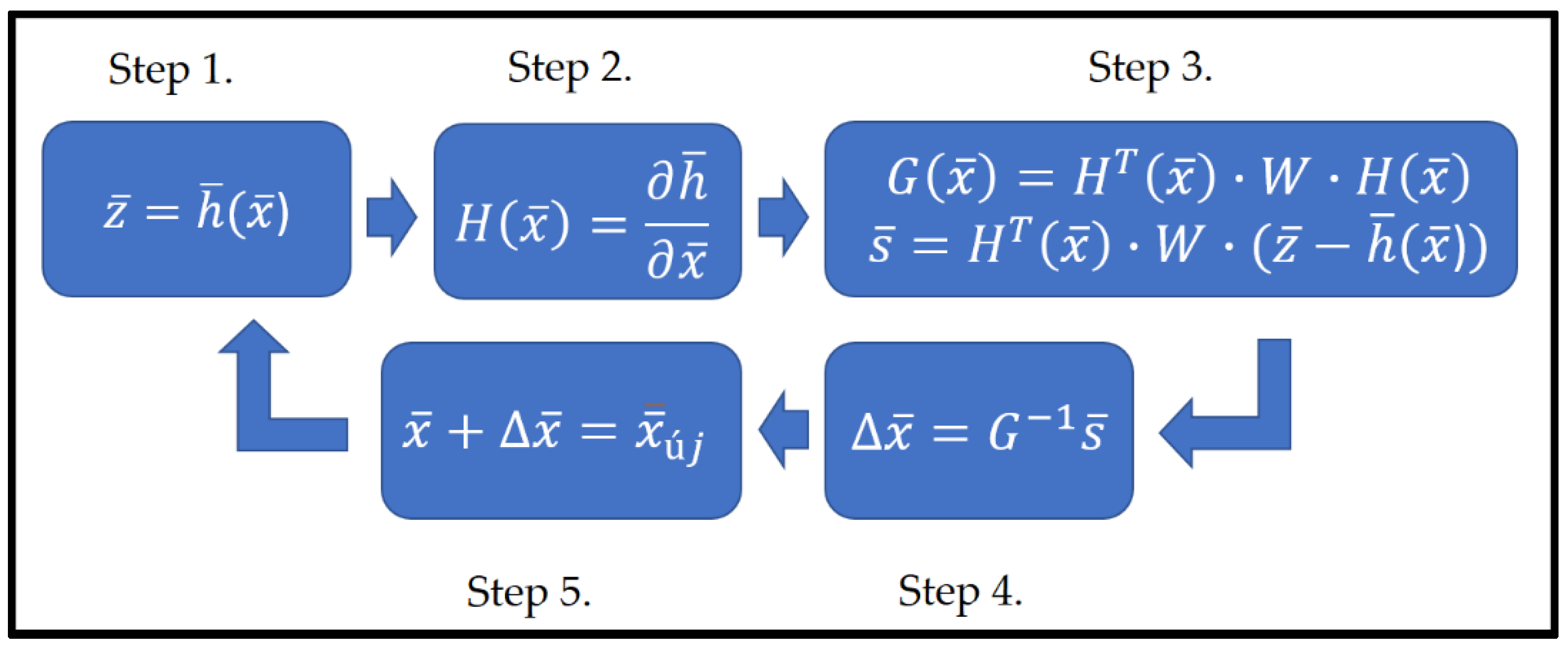
Here, a brief overview of the Gauss–Newton algorithm, used by the developed DSSE tool, is presented. The basic operation of the SE is shown in Figure 1.

To run the least square based Gauss–Newton algorithm with proper configuration settings, a network must be built as a graph. This matches the part of the workflow of network modeling in a conventional simulation software. The great advantage of the pandapower library is that, on the one hand, the building process can be fully automated; and on the other hand, in the case of possible change necessities, the software is more flexible than a network modeled using specialized software. The most influential factor that affects modeling is how input data structure is available to create the current network or subnetwork. In different cases, different file formats are used to provide the essential parameters. (From Ref. [28], it can be seen that it may be advisable to apply the dict format to store the data with IDs.) In addition, it is worth noting that these superstructures are primarily dependent on the current network.

The developed tool processes the information differently on different networks, with different formats of input parameters. However, its operation can also be characterized in general, as shown in Figure 2.

The application was designed based on object-oriented principles. The architecture of the application is hierarchical: it consists of modules and submodules in a top-down refinement manner. In this layout, the Main module controls the entire process. To show the essence of the operation, we review the above modules in the following. Configuration settings are implemented using the Configuration file [29], and a network for DSSE is created using the Network builder module. The substantive part of the DSSE is conducted in the framed part. The Measurement maker module retrieves individual measurement data and pseudo measurements from arbitrary input files. The Simulator module defines the simulation class, a mediator object controlling the entire flow of the application and coordinating object interaction [30]. The Algorithm module runs the discussed WLS algorithm, and the Validator module can check each result by running load flow. Finally, the Output writer module can save the calculated data.

2.2. Pseudo-Measurement Generation

DSSE implementations rely heavily on pseudo measurements to make the system observable. Pseudo measurements serve as a substitute for the actual data from digital consumption meter devices. They are commonly devised using historical datasets and load profiles. The proposed DSSE uses solely pseudo measurements as an input, since real-time measured load data are currently not available for the supply areas. These pseudo measurements are checked against the historical total loading of the supplying MV/LV transformer to maintain consistency. Thus, the aim of this approach is primarily not to obtain more and more precise state of the network in the presence of real but incomprehensive measurements, but to perform numerical experiments to evaluate the network models themselves and the potential accuracy in case no real-time measurements are available. (Deployment and integration of such onsite voltage and current measurements are planned in 2022. With these measurements, a greater accuracy and network observability will be assured soon).

The proposed model of pseudo measurements consists of active and reactive power values provided for each quarter-hour time period of the whole year. The pseudo-measurement database was generated from two sources: SLPs supplied by the Hungarian DSO, E.ON [31], and a collection of samples of actual active power measurements. SLPs represent a realistic consumption profile of Hungarian LV consumers and are traditionally used by the DSO for network upgrade planning and to predict electricity consumption throughout the year. The used SLPs consist of consumption rates for the entire year in a 15 min resolution and include datasets for typical residential and controlled loads. To obtain the actual consumption values, these datasets were scaled by multiplying them with the modeled consumers’ AAC. The measurement sample dataset (MSDS) was recorded in a Hungarian distribution network, and it contains electricity consumption time series datasets, characteristic of LV consumers in Hungary. The sample set contains data of 334 residential and 69 controlled consumers, each consisting of 15 min consumption values for the whole course of one year.

The created pseudo measurements represent five distinct scenarios, each with increasing levels of precision, to test the effects of measurement uncertainty on the estimation. The residential datasets are further classified into four clusters according to their energy volume. Annual consumption values were separated into 52 weeks. Odd weeks serve as input to the estimation, and even weeks as input to the load flow, whose output is regarded as a ground truth to validate the estimation. This system results in 26 weeks’ worth of simulation data.

2.2.1. Scenario Generation

For testing the effects of different levels of measurement uncertainty, five pseudo-measurement scenarios are devised, representing increasing levels of precision. The method of consumption pattern generation is identical for residential and controlled consumers. These are detailed below, using the following notations:

• $l=1,\dots ,L$ are indices of the loads of the dataset ($L=344$ for residential, and $L=69$ for controlled datasets);
• $t=1,\dots ,T$ are indices of time periods ($T=34,944$ for the whole year);
• $P_l\left(t\right)$ is the consumption value of load $l$ at time period $t$ in the original MSDS dataset;
• $p\left(t\right)$ is the SLP value for time period $t$ scaled for unit annual consumption;
• $P_{\mathrm{sc}}^l\left(t\right)$ is the consumption value of load $l$ at time period $t$ according to scenario $\mathrm{sc}$.

Method 1. All loads consume the same amount of energy in each time step. The constant consumption value is the overall average of the entire dataset.

$$P_1^l\left(t\right)=P_{\mathrm{avg}}\triangleq \frac{1}{LT}{\displaystyle \sum }_{l=1}^L{\displaystyle \sum }_{t=1}^T{P}_l\left(t\right)$$

(1)

Method 1m. SLP-based consumption, where each load consumes the same amount as the other loads at a given time step.

$$P_{1\mathrm{m}}^l\left(t\right)=P_{\mathrm{avg}}·p\left(t\right)$$

(2)

Method 2. All loads consume constant energy. This constant value is unique for each load and is the average of their annual consumption.

$$P_2^l\left(t\right)=P^l{}_{\mathrm{avg}}\triangleq \frac{1}{T}{\displaystyle \sum }_{t=1}^T{P}_l\left(t\right)$$

(3)

Method 2m. SLP-based consumption. The mean consumption differs for each load and is based on the aggregated annual consumption of the given dataset.

$$P_{2\mathrm{m}}^l\left(t\right)=P_{\mathrm{avg}}^l·p\left(t\right)$$

(4)

Method 2mm. Load consumptions directly correspond to the smart meter time series data from the MSDS.

$$P_{2\mathrm{mm}}^l\left(t\right)=P_l\left(t\right)$$

(5)

These scenarios help to distinguish between varying levels of precision in the input data, with the first scenario (1) being the least accurate, and the last scenario (2mm) being the most accurate compared to the validating dataset consisting of smart metered data. Of these scenarios, (1), (2) and (2m) are the ones used in DSO practice. Scenario (1m) would be theoretically applicable; however, due to its low accuracy in terms of estimation result, it is not covered in detail in this paper. Scenario (2mm) will be applicable in future research once smart consumption meters are deployed in these pilot environments.

2.2.2. Clustering

It is common practice to classify consumers based on their annual energy consumption. For the purpose of selecting an appropriate, characteristic time series dataset for each load of the network during simulation, residential datasets were divided into four clusters. The boundaries of the clusters are marked by the aggregated annual energy in the dataset. These boundaries were first estimated by clustering the annual consumption values of the loads for all four demo networks and the aggregated annual consumption of the original datasets using the k-means method. Then, the boundaries were set based on the heuristic analysis of the clustering results, as illustrated in

Table 1. Cluster boundaries and number of datasets in each cluster.

Boundaries of the Datasets (Aggregated Electricity (AE) in kWh)	Number of Datasets
AE ≤ 2000	167
2000 < AE ≤ 5000	104
5000 < AE ≤ 10,000	29
10,000 < AE	60

.

2.2.3. Pseudo-Measurement Uncertainty Calculation

State estimation determines the maximum likelihood network state, based on the reliability of measurements. Since measurements with a lower level of uncertainty are considered with a higher weight, it is essential to set the uncertainties realistically.

Uncertainty was calculated for each scenario as the mean of relative difference between the scenario consumption and the reference dataset consumption.

$$u_{\mathrm{sc}}=\frac{1}{LT}{\displaystyle \sum }_{l=1}^L{\displaystyle \sum }_{t=1}^T\frac{P_{\mathrm{sc}}^l\left(t\right)-P_{\mathrm{ref}}^l\left(t\right)}{P_{\mathrm{ref}}^l\left(t\right)}$$

(6)

where

• $u_{\mathrm{sc}}$ is the uncertainty of scenario $\mathrm{sc}$;
• $P_{\mathrm{sc}}^l\left(t\right)$ is the power consumed by load $l$ at time $t$ according to scenario $\mathrm{sc}$ for odd weeks;
• $P_{\mathrm{ref}}^l\left(t\right)$ is the reference power consumed by load $l$ at time $t$.

These values are the original smart metered consumption values of even weeks.

The obtained values are seen in

Table 2. Uncertainty values of residential and controlled datasets for the scenarios.

Scenario	${\mathit{u}}_{\mathbf{sc}} \mathbf{of} \mathbf{Residential} \mathbf{Loads} (‰)$	${\mathit{u}}_{\mathbf{sc}} \mathbf{of} \mathbf{Controlled} \mathbf{Loads} (‰)$
1	2.54047	123.225
1m	2.53925	123.146
2	0.884116	119.048
2m	0.940834	119.195
2mm	0.275357	127.572

. There are two orders of magnitude difference between the uncertainty of residential and controlled loads, which is due to the intermittent nature of controlled consumption. This is explained, for example, by the fact that a significant proportion of consumers have water boilers, and their behavior is difficult to estimate.

2.2.4. Matching the Datasets to Loads of the Network

During state estimation, each load of the network is randomly paired with a dataset from the pseudo-measurement database, taking into consideration whether it is a residential or a controlled one. Each residential load’s dataset is selected from the cluster whose consumption boundaries match the AAC of the load (load AACs are obtained from the network input data). The same method is applied for the input data of the load flow validation, with the exception that this input is selected from even week time periods, while DSSE input is from odd weeks.

During the process of state estimation, measurements are defined for network nodes instead of individual loads; thus, measurement values corresponding to the same network node are aggregated. The uncertainty of the aggregated measurement was defined as a sum of the uncertainty of individual load measurements, employing a Gaussian Mixture Model.

2.3. Topology and Inputs

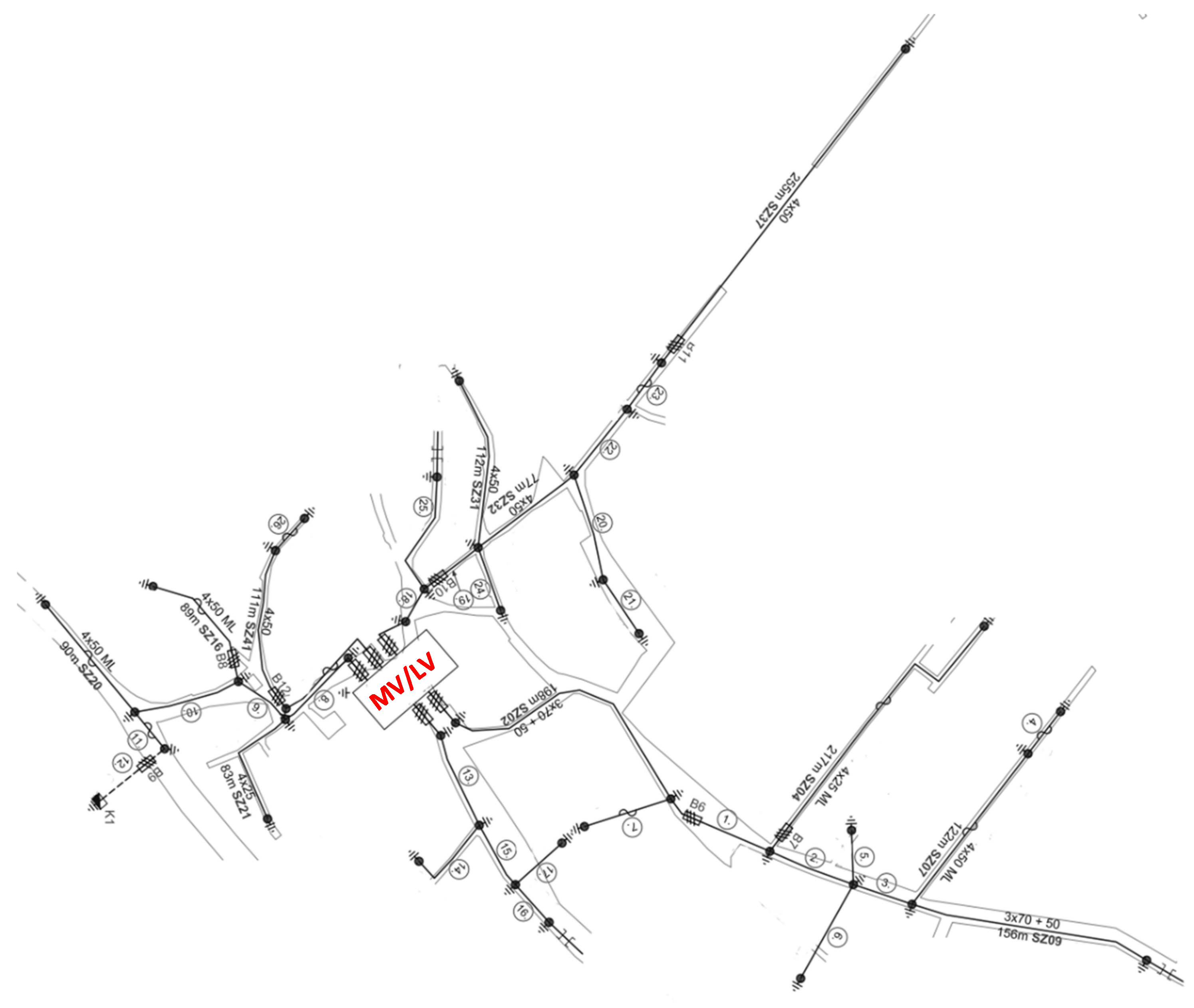
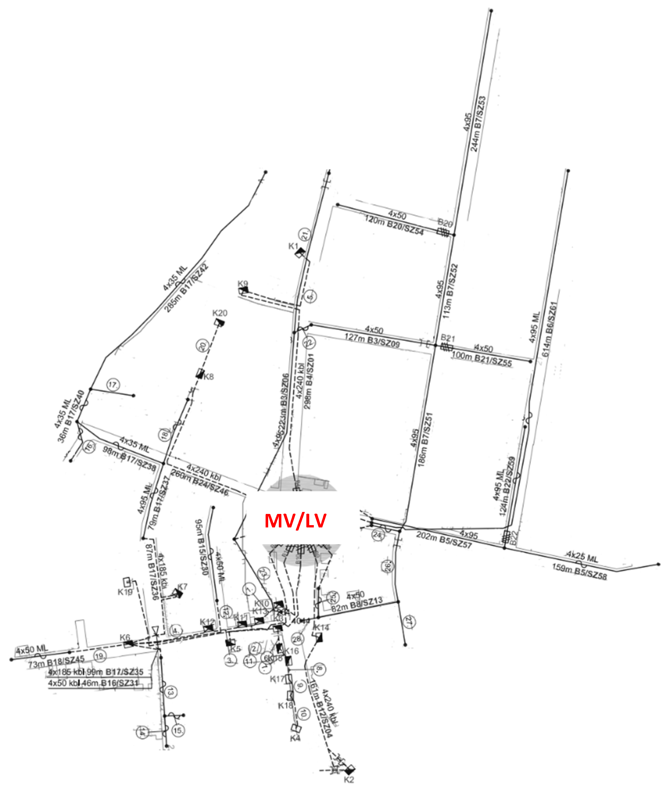
The modeled supply areas belong to the LV distribution network of western Hungary. Every area is modeled using an external grid element, a MV/LV transformer and all the elements from its LV side. The numbers denoting these areas are 18,680, 20,667, 44,333 and 44,600, consisting of 2, 4, 5 and 10 circuits, respectively. Topologies of the supply areas are shown in the Appendix A (see Figure A1, Figure A2, Figure A3 and Figure A4). In all four cases, modeling essentially involves the building of three representations with different load placement accuracies, for practical reasons. E.ON stores the descriptive characteristics of these transformer areas in two ways. The first way is to use AutoCAD files with an *.dwg extension, and the second is to use the INIS system, from which the data can be exported on demand to Excel files. The first is the construction of the fully accurate model, but its disadvantage is that the network cannot be assembled from it automatically, so modeling must be carried out manually. The second contains approximations and simplifications. For example, it is possible that certain buses are neglected, or consumers and lines specified with Unified National Projection (UNP) coordinates are not actually in the defined position. However, the system can be created fast from this second dataset using the queried Excel files. Thus, the three representations with different levels of precision in terms of load placement built from these data are:

• the system defined by the AutoCAD files with *.dwg extension,
• the data-driven system that can be defined by Excel queries from INIS,
• and the more precise data-manipulated system that can be defined by Excel queries from INIS.

Of all the system types, the manually built one (referred to as the AutoCAD model) requires the fewest hardware resources, and it is the least challenging in a professional sense, as one does not need to understand the details of the structural elements of the INIS query. However, this simplicity cannot be declared in terms of human resources. The examined four supply areas together contain more than a thousand consumers. These and the connected lines, buses, switches and circuit breakers had to be represented one by one. In addition, the markings in the *.dwg files were not always clear regarding which line belonged to which circuit, and due to the redundancy with the initial INIS query, continuous consultation with E.ON was required. In addition, the support of Google Street View and E-közmű [32] tools were used, and on-site checks were also performed.

The system that can be defined by Excel queries from the INIS system (referred to as the INIS model) consists of fifteen files: (1) the consumers file, (2) the recently connected consumers file, (3) the AAC data file, (4) the file of buses with connection data, (5) the file of buses with coordinates, (6) the file of switches with connection data, (7) the file of switches with coordinates, (8) the file of circuit breakers with connection data, (9) the file of circuit breakers with coordinates, (10) the transformer location data file, (11) the file about the technical parameters of the transformer, (12) the file of the lines, (13) the file about the location data of the lines, (14) the file of the assistant lines and (15) the file about the location data of the lines behind the meters. An input reader script was created using the openpyxl module to build all four areas. Each network is built as follows. The types of lines are defined first, and then, the file containing the location data of the lines can be examined in parallel with the file of the lines. From the first one, the unique ID and the UNP coordinates of each bus can be extracted, and from the second one, the line types can be read. Consumer IDs, the types, and IDs of the objects where the consumers are connected, and the UNP coordinates, are available from files belonging to the consumers. Finally, by opening all but the first three of the fifteen files and recursively searching for each connected object, the network can be built, and clear consumer-line assignments can be specified. UNP coordinates are required because in the INIS data structure, consumer-line pairs are defined. Thus, in each case, based on the distance data, it can be decided to which end of the line the given consumer can be connected.

This INIS query was refined as follows. Typically, in the INIS registry, as it was mentioned earlier, some buses are not created. In this case, the consumers connected to these buses will be connected elsewhere. (In practice, some lines are merged in the INIS data structure, and each of their consumers are connected to the endpoints of the merged lines.) According to the standard method of E.ON, the following process is carried out using the contribution of the company’s internal Neplan-Excel conversion as well. E.ON DSO’s LV grid mostly consists of overhead lines. The database of the DSO currently does not contain information on the individual poles, only the line segments, though customers are always connected to the networks at poles. The DSO possesses geographical data on the position of the customer’s consumption meter from the periodic readings or the installation of new meters. Therefore, creating segments with the length of the usual distance between poles offers a possibility to estimate the connection point of customers with the assumption that the customer is connected to the nearest ‘virtual’ pole. This method reduces the error of the voltage profile and loading estimation, as the distribution of the loads and generators are closer to the actual positions, while it does not require the process of any connection plans. To achieve this, the line segments in the examined network are scanned continuously, one after the other, and their length is checked. If it is below 50 m, it can be assumed that a line segment of this length between two poles can exist, so the algorithm continues the iteration to the next line. However, for line segments longer than this, the scanned length is divided by 30 m as the typical pole distance. Thus, an approximate number of pieces can be obtained for how many line segments the given element can actually consist of. The algorithm calculates the floor and the ceiling of this approximate number, from which it is advisable to choose the one that results in a segment length closer to 30 m. Thus, in the case of l_f, the line will be divided by the floor of the approximate number; and in the case of l_c, the line will be divided by the ceiling of the approximate number, and each consumer will be connected to the nearest bus. This algorithm (referred to as manipulated INIS model) is shown in Figure 3, where the red arrow indicates the case where manipulation is required due to a line longer than 50 m.

It must be emphasized that this approach does not neglect any element of the network itself but the connection between the LV branch and the point of delivery. This situation is usually also handled by the planning principles of the network (as there is a difference between the prescribed voltage limits for the LV branch and the point of delivery—currently 2.5% of nominal voltage in Hungary). These short lines (typically only a few meters) connect the customers as parallel elements; therefore, they do not alter the electrical attributes of the network significantly, which is accessible at the DSO information systems. This method—which is based on the modeling approach currently used by the DSO as well—can be automated and assigns the customers to the ‘virtual’ poles to assume the loading distribution accurately.

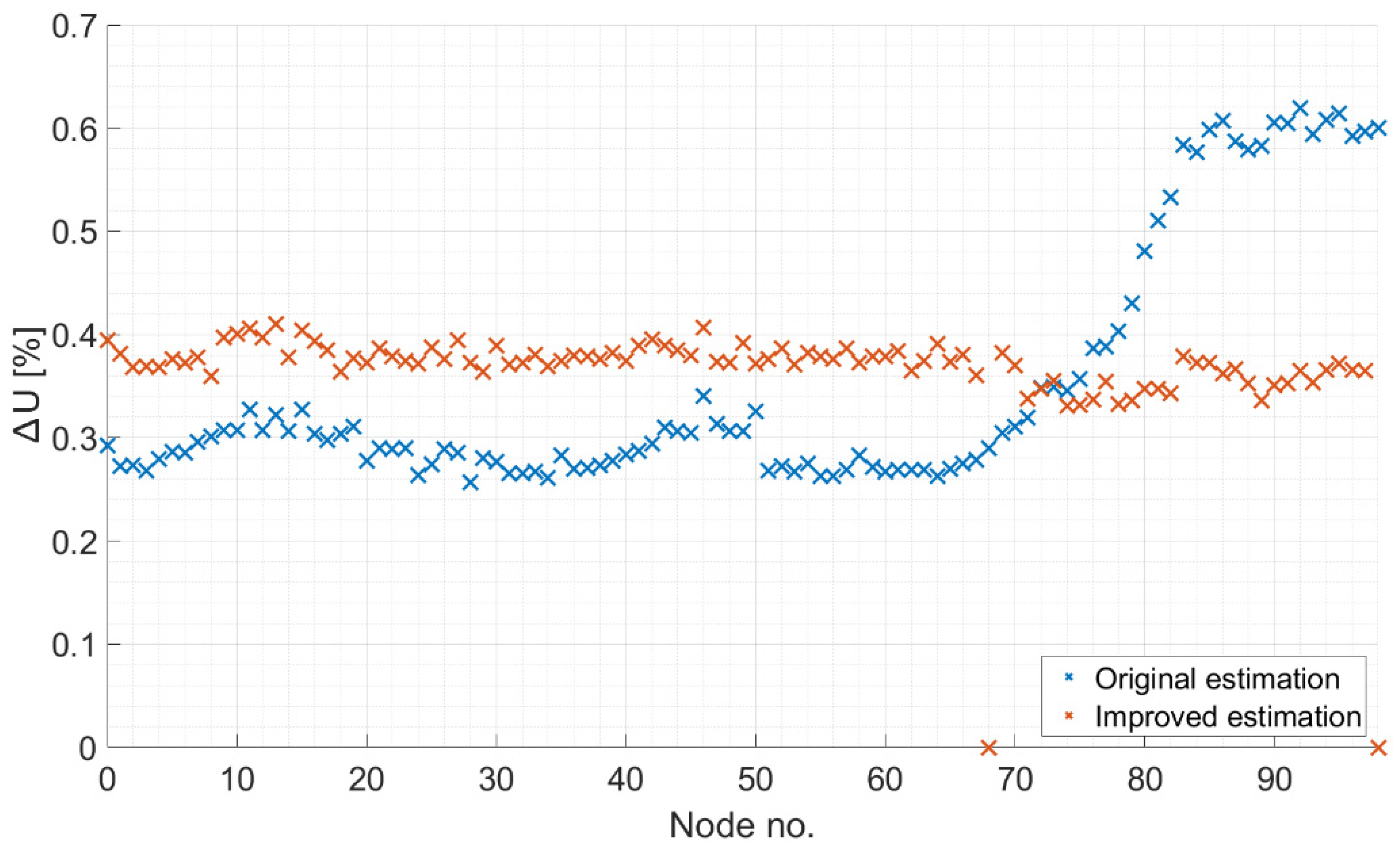
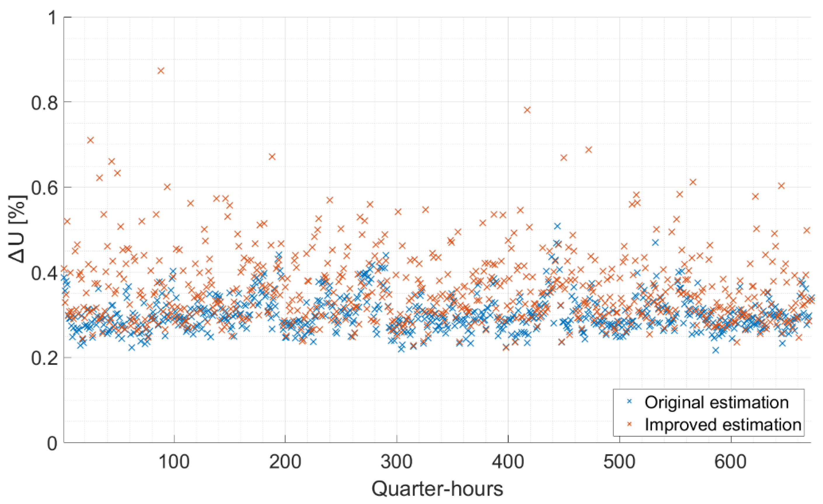
The initial parameters that can be used for modeling, but have not always been used, were the AAC and a typical LV annual consumer profile per connection. Of course, these profiles do not exactly describe the specific consumer, but they can give a good approximation in terms of modeling. The 18,680 network consists of two circuits and predominantly conventional loads. Here, DSSE was performed for each scenario and for each load model to provide a detailed analysis. The relative error of voltage magnitudes was calculated as follows:

$$\Delta u=\frac{U_{estimated}-U_{load flow validated}}{U_{load flow validated}}$$

(7)

3. Results

In this section, the results of Method 1 and the better results of Methods 2 and 2m can be seen. With the better estimations, the three networks with different levels of precision in terms of load placement are also presented. Finally, a correction method is demonstrated with Method 2m.

3.1. Comparison of the Modeling Methods and Load Placement Techniques

Figure 4 shows Method 1 where neither individual AAC nor SLP were used. In this case, AAC is interpreted to be equal over the entire area, and a uniform distribution is assumed. AAC per consumer is used in Figure 5, and AAC and SLP per consumer is used in Figure 6.

Figure 4 shows that using the simplest consumer models, the average relative error on the smallest network can climb to almost 3%. Here, spatial homogeneity means that each load consumes the same amount as the other loads at a given time step, and temporal homogeneity means that all loads consume the same amount of electricity in each time step. In the case of larger networks, this error may reach even higher values because of the trend that buses more distant from the supplying MV/LV transformer have bigger relative errors. Therefore, it seems necessary to use a more accurate model, considering the unique AAC values as well.

It can be seen from Figure 5 and Figure 6 that the relative errors in the voltage magnitude estimations have been significantly reduced, especially when SLPs were also used. Comparing the manually built AutoCAD models to the automatically generated and refined INIS models, important differences are seen. Typically, the automatic structure results in a different numbering for each bus, but by resolving this contradiction essentially, the estimation results are in the same range. The most accurate is, of course, the manual model, but the manipulated INIS model is also definitely an improvement over the original INIS query. The numerical results are also convincing from the aspect of future industrial application because the automated network generation was able to handle all networks defined in the same INIS format. Considering the human resource needs of manual modeling, the use of the refined INIS model is advisable.

3.2. Accuracy Correction

For Areas 44,333 and 44,600, a correction technique is presented that can reduce the offset component of the relative error to less than 0.5%. The essence of the method is that in practice, although the use of pseudo measurements is a good and efficient alternative for better LV network monitoring, it is worth integrating real measurements into the DSSE method. A total of 1933 iterations were run in connection with the estimations. These made it possible to identify those buses in the networks that give the closest estimation error to the offset error by test estimations on a separated dataset. So, if measurement devices are placed on these buses, even a moderate number of them is enough to significantly improve the accuracy of DSSE.

The place of the first measurement device is the bus that best approximates the average error to eliminate offset. To find this bus, a separate pseudo-measurement dataset was used. From this dataset with multiple DSSE run, a set of relative error data was procured. By grouping this data by bus, it was possible to identify the bus with error closest to the average relative error. The place of the second measurement device is one of the endpoints of the network, where the estimation accuracy is expected to be the lowest. Experience has shown that it is worth correcting the estimations of the buses closer to the transformer with the estimations created for the first bus and that the correction between this point and the endpoint must be made according to the ‘lever rule’. In line with this, the correction given by both points must be used in inverse proportion to the ‘test point distance’ from them. This ‘distance’ basically equals the impedance between the bus and the transformer, which can be replaced by the difference in the bus indices of the given circuit if the variance of the differences between the pylon distances is not extraordinarily large.

The calculated correction and the applicable approximation are described in Equations (8) and (9). The essence of the correction is that buses close to each other have similar relative errors. Thus, if real measurements are available on bus ‘a’ and bus ‘c’ bus, the estimation for bus ’b’ can also be corrected. The correction is proportionally more affected by the difference between the real measurement and the estimation of the closer bus and less affected by the difference between the real measurement and the estimation of the further bus. This method is widely used in other sciences, such as materials science [33].

$$\Delta U_n=\frac{\Delta U_v·(Z_n-Z_b)+\Delta U_b·(Z_v-Z_n)}{(Z_v-Z_b)}$$

(8)

$$\Delta U_n\approx \frac{\Delta U_v·\left(n-b\right)+\Delta U_b·\left(v-n\right)}{v-b}$$

(9)

where

• b is the index of the inside bus that best approximates the average error;
• v is the index of the endpoint bus;
• n is the index of the bus to be corrected;
• ∆U_i is the correction of the bus with index i;
• Z_i is the impedance of the bus with index i calculated from the transformer.

Using these equations, tests were carried out for Areas 44,333 and 44,600. The most suitable location for the placement of the measurement device was bus 51 for Area 44,333 and bus 68 for Area 44,600. In both cases, these are inside points in the longest circuit in the given supply area. It can be seen on Figure 7 and Figure 8 that the algorithm is successful for both networks, so the estimation error remains below 0.5%. This is very favorable, as in the case of a network of 70–100 buses, a good approximation of its state can be given with the help of two well-placed measuring devices, pseudo measurements and the appropriate DSSE algorithm.

3.3. Temporal Effect of Accuracy Correction

The temporal accuracy of the estimations is illustrated in Figure 9 for Area 20,667.

Here, the estimation and validation results of each quarter-hour time window for each test week were saved, and the average relative errors were calculated accordingly. Figure 9 illustrates the average estimation error of the network with the developed algorithm and correction. This correction may increase the average error for the entire supply areas but keeps it below 1% for all four cases, thus eliminating very erroneous estimations and reducing the deviation of the absolute value of errors per bus. More detailed examination of the correction method, especially the proper identification of the bus, which is to be used for the correction, will be carried out by the authors.

3.4. Summary of the Results

The temporal and spatial averages of the three detailed and the theoretically applicable scenarios for the complete dataset are given in

Table 3. Temporal and spatial averages of the relative errors of the scenarios.

Method	Load Placement	18,680	44,333	44,600	20,667
1	INIS	1.43	1.84	2.09	0.76
	Manipulated INIS	1.52	1.83	2.43	1.31
	AutoCAD	1.69	1.72	2.96	2.56
1m	INIS	1.52	2.13	2.11	0.92
	Manipulated INIS	1.61	2.01	2.14	1.57
	AutoCAD	1.80	2.00	1.91	3.09
2	INIS	0.39	0.45	0.34	0.17
	Manipulated INIS	0.40	0.45	0.36	0.25
	AutoCAD	0.38	0.44	0.41	0.41
2m	INIS	0.33	0.39	0.30	0.12
	Manipulated INIS	0.34	0.38	0.31	0.17
	AutoCAD	0.32	0.38	0.35	0.26

.

4. Summary

An LV DSSE tool was developed and proposed in this paper, focusing on the critical aspects of finding accurate and coherent information on network topology with automated management of information systems, real LV network implementation for power flow calculation and managing portions of the network characterized by uncertain or inconsistent line lengths. Using pandapower and the Gauss–Newton algorithm, SE were run in four Hungarian LV supply areas. For testing the effects of different levels of measurement uncertainty, different pseudo-measurement scenarios were defined with different combinations of AAC and SLP usage. A 50–50% (odd week–even week) estimation–validation split was applied for each scenario to run from the dataset of 52 weeks. For all four networks, modeling was performed with three different load placement accuracies, due to the data storage method of the DSO. In this regard, an INIS model refining algorithm was implemented to find a balance between reducing human resources and achieving accurate estimations. The presented method is able to estimate node voltages with a relative error of less than 1% in case of using AACs. A meter-placement method is published as well to reduce the maximum value, and this way, the deviation of the absolute value of errors per node is reduced. The main conclusion of the paper is that the usage of AACs and SLPs, as well as optimal meter placement, can be a significant step toward real-time network monitoring.

Future research will focus on the extension of the presented approach toward more realistic scenarios. Pseudo measurements will be partially replaced by real measurements from actual metering devices, and the rest of the measurements will be yielded by load-flow calculations to ensure a plausible load configuration model. The validation procedure will also be extended to include load-flow results from the same dataset as reference.