Dealing with Low Quality Images in Railway Obstacle Detection System

Abstract

Object recognition and classification as well as obstacle distance calculation are of the utmost importance in today’s autonomous driving systems. One such system designed to detect obstacle and track intrusion in railways is considered in this paper. The heart of this system is the decision support system (DSS), which is in charge of making complex decisions, important for a safe and efficient autonomous train drive based on the information obtained from various sensors. DSS determines the object class and its distance from a running train by analyzing sensor images using machine learning algorithms. For the quality training of these machine learning models, it is necessary to provide training sets with images of adequate quality, which is often not the case in real-world railway applications. Furthermore, the images of insufficient quality should not be processed at all in order to save computational time. One of the most common types of distortion which occurs in real-world conditions (train movement and vibrations, movement of other objects, bad weather conditions, and day and night image differences) is blur. This paper presents an improved edge-detection method for the automatic detection and rejection of images of inadequate quality regarding the blur level. The proposed method, with its improvements convenient for railway application, is compared with several other state-of-the-art methods for blur detection, and its superior overall performance is demonstrated.

1. Introduction

One of the most important problems that arise in autonomous driving systems is the recognition and classification of objects as well as the calculation of the distance to them. This problem is particularly pronounced in the railway, resulting in delayed braking and train-to-obstacle collisions. It has been demonstrated that the adoption of machine vision algorithms can significantly improve such a situation. Typically, a series of sensors, cameras or radar are positioned at the locomotive’s front end to capture real-time circumstances in front of the train, and the recorded material, in the form of videos and photos, may subsequently be examined to assess the current situation using image processing algorithms [1,2]. Based on this information, a scenario evaluation can be issued to the autonomous driving system to assist it in making a prompt decision. However, among all of these videos and images captured by camera sensors, there will certainly be a percentage of images that are not of sufficient quality for further use. Distinguishing between images of high perceptual quality and distorted ones in a subjective way is burdensome for humans and unfeasible in real-time applications. Therefore, the development of image quality estimation techniques for automatically finding high-quality images is gaining more and more attention.

All over the world, the automation of the railways is an ongoing process, essential for improving the quality, capacity, energy efficiency, flexibility, cost-effectiveness, and, above all, safety of the railway traffic [3,4,5]. One of the most important problems for building autonomous operating railways, these days, is designing a safe and reliable obstacle detection (OD) system [2], which is exactly one of the main goals of the SMART1 and SMART2 projects (SMart Automation of Rail Transport), funded by the Shift2Rail Joint Undertaking under the European Union’s Horizon 2020 research and innovation program [6,7]. The SMART1 project delivers a prototype of an on-board long-range all-weather OD and a track intrusion detection (TID) system for the mid-range (up to 200 m) and long-range (up to 2000 m) detection of potentially dangerous objects on the train’s path as well as short-distance wagon recognition for shunting onto buffers. SMART2 further builds on the achieved results by developing new hardware solutions and software algorithms for object detection, mainly by adding two more systems—advanced trackside and airborne OD&TID—and by integrating all three systems into one via interfaces to the central decision support system (DSS). In such a way, the autonomous OD for railways achieves an increased detection area, including areas behind curves, slopes, tunnels, and other elements blocking the train’s view on the rail tracks, in addition to a long-range straight rail-tracks OD. Sensors of the three systems (on-board, advanced trackside, and airborne) are used to inform DSS about possible obstacles and track intrusions in their fields of view, and DSS then makes the final decision about class and distance to the obstacle and informs the train control systems.

The equipment utilized in the implementation of the SMART2 project activities includes RGB, thermal, and high-performance vision SWIR cameras besides other sensor types. Cameras generate image files in RAW format containing all pixel data captured by a camera’s sensors and holding all the information recorded by the imaging chip without any loss. Raw data enable full control and fine-tuning of picture parameters, such as brightness, saturation, color, exposure, and contrast. Raw formats are especially suitable for shooting open-space photos, where various lost details can be recovered in extremely dark or bright areas. On the other hand, the major drawbacks of the raw files are their size and the need for specially tailored graphical software packages, required for editing them. The other option for the cameras is the possibility to save the images in the most common digital image format, JPEG, which uses the method of lossy compression, thus making a trade-off between storage size and image quality. JPEG is also good for representing open-space scenes, where it can typically achieve 10:1 compression with little perceptible loss in image quality. The backbone of JPEG compression is discrete cosine transform, a mathematical operation which converts video material from the spatial (2D) domain into the frequency domain.

It is well known that when images are captured in real-world outdoor conditions, they are frequently subject to a variety of disturbances and factors, resulting in lower image quality. After analyzing the real-world images of railway scenes with obstacles captured by thermal and RGB cameras, we discovered that, of all the distortions that can have a negative impact on image quality (e.g., vignetting, lateral chromatic aberration, and noise), blur occurs on the largest number of distorted images. Blur generally occurs when an image is captured in an out-of-focus situation (out-of-focus blur) or due to motion (motion blur), or when some other disturbance occurs during image manipulation procedures (more detailed explanation is given in Section 2). Motion blur in railways often arises because the train is moving and the objects around it are static, or in situations when the camera moves for some reason at the moment that the picture is taken (e.g., vibrations, and train shaking) [8]. In addition, blur can also be produced by the movement of the observed objects in front of the train. On the other hand, out-of-focus blur is caused by the differences in train speed and camera focus. This distortion in the images can lead to the lack of clarity that will later decrease the accuracy rate of the whole system. In order to significantly reduce or even prevent the motion blur effect in images, cameras are mounted on gimbals to suppress vibrations transmitted from the moving vehicle, as well as to allow the rotation of cameras and on-line control of their orientation so as to follow the tracks reliably [9]. Furthermore, the cameras are mounted in special housing, which is vibration isolated [10] to lower the level of camera vibrations. Despite the implementation of these solutions, motion blur is still present in a certain number of images. On the other hand, the RGB cameras are zoomed to cover the distance necessary for the railway onboard OD and TID (up to 2000 m), which contributes to the existence of out-of-focus blur in images. Thus, this paper will focus on blur distortion.

The collected images are to be used within the OD module to train the neural networks which are directly responsible for obstacle detection [11]. The efficiency of the deep learning systems is strictly correlated with the quality of the training dataset. A high-quality training dataset improves the inference accuracy and speed while consuming fewer system resources and speeding up the learning process. Having this in mind, the recorded images used for the training purposes must be of good quality. The main goal of the algorithm proposed in this paper is to assess image quality and reject images that do not meet certain criteria. In this way, low-quality images in the database can be automatically labeled and separated from high-quality images for later re-use. Moreover, the same functionality can be used for the automatic rejection of images from the processing pipeline in order to preserve computational time, which is a critical resource due to real-time requirements. All the developed systems (including OD, TID and DSS) operate by using certain deep learning systems which provide excellent results; however, even with the use of modern computers, they are still a quite time-consuming option. In order to avoid further complications of the overall system’s functionality and save time, the blur detection (BD) problem needs to be addressed by an algorithm which will satisfy requirements with regard to simplicity, computation time, and accuracy.

Many studies, which will be discussed in more detail in Section 3, are particularly interested in the BD problem because blur is one of the most significant distortion types in images. The solution to this challenge could be the beginning of a de-blurring procedure or some other form of picture processing, but the focus in this paper is exclusively on blur and non-blur image classification. The existing literature on this topic shows that among the many approaches, three groups of blur approaches can be distinguished: frequency-based, edge-based, and depth-based methods. We achieved the best overall results using BD based on the Laplace operator, which seems to be an ideal candidate that satisfies all the previously specified requirements. Certain practical challenges were handled during the project by upgrading the existing method and introducing new functionality. The main disadvantages regarding inappropriate results in the presence of noise and the manual selection of the threshold were overcome by implementing our own solutions which are elaborated in Section 4.

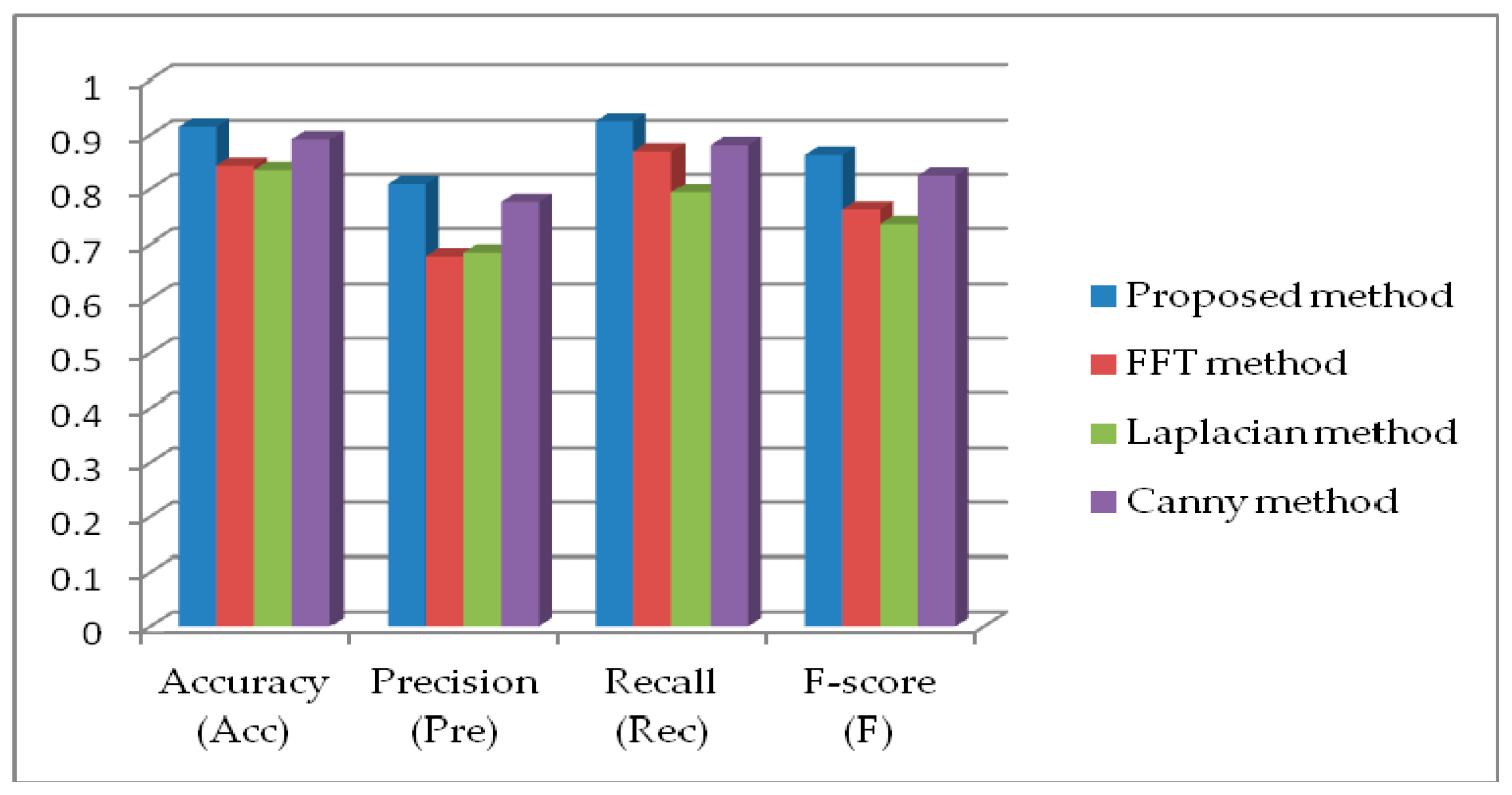
At the end of the paper in Section 5, we evaluate our proposed algorithm using real-world images of railway scenes with obstacles and compare the obtained results with several other state-of-the-art methods. We select different methods which belong both to the group of edge-based and frequency-based algorithms and conduct an analysis by comparing the relevant parameters such as precision, accuracy, recall, and F score. It is shown that the proposed method gives the best overall results in the railway application for each of the proposed evaluation measures. Finally, the results of the evaluation of the performance of different approaches using the real-world railway dataset are presented in the form of a precision recall curve, which also favors the proposed method.

In summary, the major contributions of the proposed paper are as follows:

(i)

We proposed an improved Laplacian-based edge detection algorithm for blur detection;

(ii)

The main disadvantage of the edge-detection algorithm regarding the manual setting of the threshold was overcome by introducing the automatic selection of threshold values;

(iii)

We implemented the proposed algorithm in real-case scenarios in the railway application for obstacle detection;

(iv)

We improved the performance of our algorithm even further by selecting separate thresholds for day and night images;

(v)

Rigorous experiments were performed against several state-of-the-art methods over our own real-world railway dataset to prove the effectiveness of the proposed algorithm.

2. Blur in Images

To successfully design an adequate algorithm for blur detection, it is critical to comprehend the underlying concept behind the blurring distortion. Blurring is one of the most common types of image distortion in photographs and represents a shape or an area in an image that cannot be clearly seen because it does not have a clear outline or because it moves very fast, in the case of video material. Practically, blurring is the attenuation of high frequencies, which affects the frequency spectrum of the image.

Depending on the conditions under which the image blur occurs, we can distinguish between two types: motion blur and out-of-focus blur. The first type of blurriness, motion blur, presented in Figure 1b, occurs as a result of either the movement of an object in the camera’s field of vision during shooting, or the movement of the camera itself. Within this type of blur, we can also distinguish between global and local blur (spatially varying blur). Global blur occurs when the scene is static, and blurring occurs as a result of camera movement during the exposure process, while local blur occurs as a result of the movement of individual objects while other components are static. In the second type (out-of-focus blur), blurring occurs as a result of insufficient camera focus during exposure to objects of interest (Figure 1c). Insufficient focus may be due to inadequate handling of the equipment or its design, e.g., poor quality lenses and sensors. Of course, there is also the possibility of the simultaneous combination of conditions that lead to blend blur. All the above situations are common in railway case studies.

In [12], it is shown that the blurring process can be defined as

$$B=A\otimes k+n,$$

(1)

where B represents the blurred image, A is the clear image, ⊗ denotes the convolution operator, 𝑘 is the blur kernel, and 𝑛 corresponds to the noise. Blur kernels are strictly correlated with the blur type, so, for instance, a mathematical model of motion blur in the form of a line can be represented by the following kernel:

$$k_{\mathrm{motion}}\left(x,y\right)=\left\{\begin{array}{l}\frac{1}{L}, \mathrm{if} \sqrt{x^2+y^2}\le L, \tan \theta =\frac{y}{x}\\ 0, \mathrm{else},\end{array}\right.$$

(2)

where x and y denote the horizontal and vertical coordinates, respectively. L represents the blur scale, and θ is the blur angle. It should be noticed that the sum of all the elements of k is 1.

In a similar way, by implementing kernel

$$k_{\mathrm{defocus}}\left(x,y\right)=\left\{\begin{array}{l}\frac{1}{\pi R^2}, \mathrm{if} x^2+y^2\le R^2,\\ 0, \mathrm{else},\end{array}\right.$$

(3)

we can describe the mathematical model of out-of-focus blur in the form of a disk, where 𝑅 is the blur scale.

It is obvious that the mathematical model of a blend blur kernel can be obtained by convolution of previous blur kernels (2) and (3) in the form of

$$k_{\mathrm{blend}}=k_{\mathrm{motion}}\otimes k_{\mathrm{defocus}}.$$

(4)

The automatic detection and classification of blurred images or their parts can be considered as part of the blur elimination (de-blurring) process in the form of image quality assessment for further improvement processes. If there is a mathematical description of how the image was blurred, then the de-blurring method becomes easier. When there is no mathematical explanation of how the image became blurred, different methods can be used to estimate the blur. 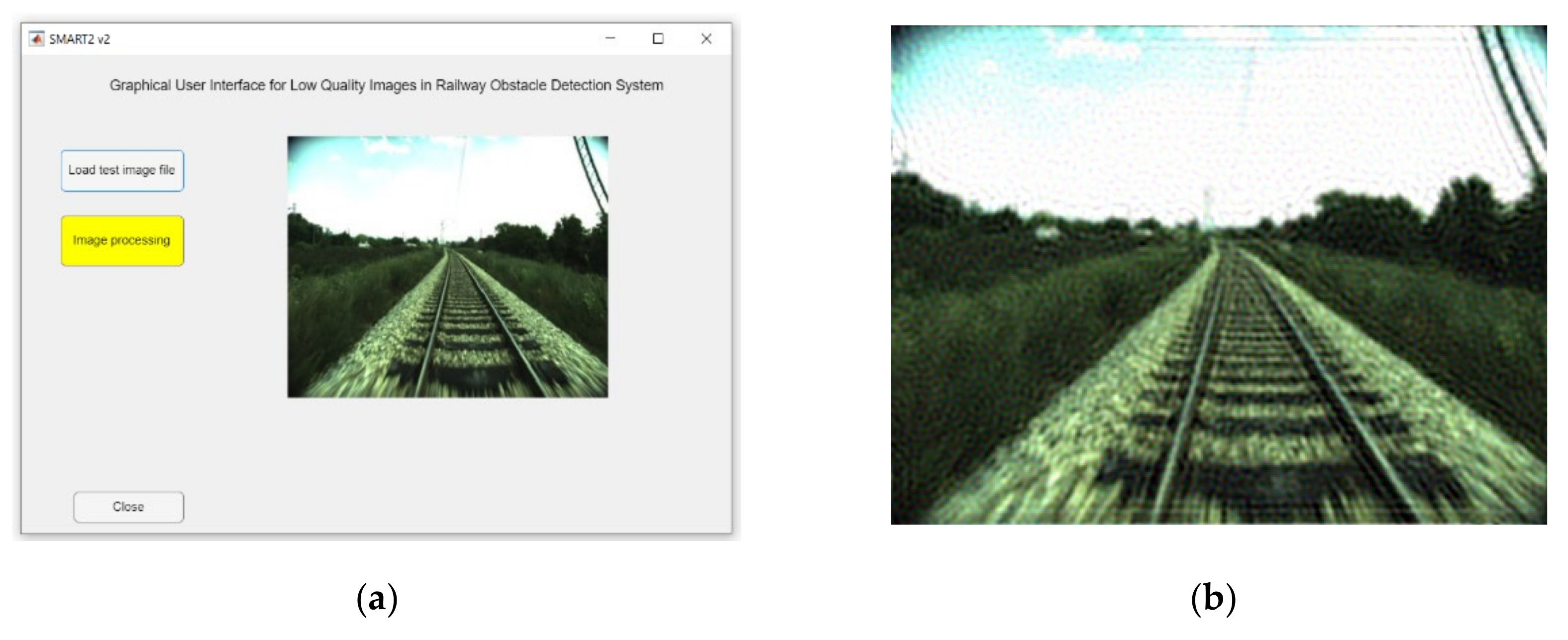Figure 2 shows an example of the created graphical user interface developed in AppDesigner from MATLAB for the de-blurring process using a pseudo-inverse filter for image restoration. Test images can be loaded, and image processing techniques for de-blurring can be applied.

It was noticed that the obtained results are mostly inadequate, which is why this paper emphasizes the segmentation of BD of the image or its parts and its classification into two categories: blurred and non-blurred. Besides the railways, this approach may be of interest in various areas where there is a direct image manipulation, such as image segmentation, object detection, scene classification, image quality assessment, image restoration, photo editing, etc.

3. State-of-the-Art Techniques for Blur Detection

The increased transmission of multimedia contents through the internet and mobile networks has made the quality monitoring of multimedia data an important topic. The evaluations obtained directly from human viewers are the most reliable for assessing the quality of multimedia data. Subjective scores or mean opinion scores are terms used to describe the findings of this evaluation. Several human viewers under controlled test conditions are necessary to obtain these scores. As a result, subjective scores are unsuitable for use in real-time applications because they imply extensive and tedious work.

Another option is to use some objective metrics to automatically rate image quality. Image quality assessment (IQA) approaches can be divided into three categories based on whether the undistorted image (reference image) or information about it is available: full-reference (FR-IQA), reduced-reference (RR-IQA), and no-reference IQA (NR-IQA). FR-IQA algorithms require as input not only the distorted image, but also a pristine (clean) reference image with respect to which the quality of the distorted image should be assessed [13,14]. However, because obtaining reference photos to measure image quality is not always possible, it is critical to establish an objective quality assessment that correlates well with human perception without the need of a reference image. As a result, more effort was put into the development of the most realistic scenario of objective-blind or NR-IQA, where image quality has to be estimated without any reference image [15,16]. If a system possesses some information regarding the reference image, but not the original image itself, the developed algorithms belong to the RR-IQA scenario [17,18]. Having in mind that the BD problem is of particular interest in this paper, and that we do not have a reference image, in the rest of this section, we describe state-of-the-art algorithms related to the blur assessment with no reference.

Based on the available information about camera settings, blur image detection (BID) can be divided into single-image and multi-image detection. While in multi-image detection, it is necessary to have additional information regarding blur densities, blur type, used sensors, etc.; single-image detection can be used without any prior information about the camera settings. Although there are numerous methods for detecting blur described in the literature, the majority of existing BID approaches can be classified into three main categories: frequency-based, depth-based, and edge-based methods [19].

3.1. Frequency-Based Methods

The most common frequency-based method examines the distribution of low and high frequencies using some variant of the fast Fourier transform of the image. The image can be regarded as being blurry if the number of high frequencies is low. High frequencies are related to the dynamic image with a lot of edges and great color differences of neighboring pixels. However, distinguishing what constitutes a low number of high frequencies and what constitutes a high number of high frequencies can be difficult, leading to subpar results when judging whether or not a picture is blurry. When a low value is utilized, images may be categorized as blurry when, in fact, they are not. On the other hand, when the threshold is set too high, images may be mistakenly labeled as clear when they are not. The authors of [20] described a method for assessing no-reference blur in natural images. The presented method uses information derived from the power spectrum of the Fourier transform to estimate the distribution of low and high frequencies. To categorize photos as blurred, an image blur quality evaluator is created by applying a support vector machine (SVM) classifier. Ref. [21] presented yet another way of employing SVM for BD. In that paper, a blur identification problem is described as a multiclass classification problem that can be handled using SVM for both horizontal motion blur and atmospheric turbulence blur. In [22], a novel method for detecting motion-blurred regions is described. The approach for estimating motion direction on blurred images provided here is based on measuring the lowest directional high-frequency energy. The collected findings revealed that the proposed strategy improved accuracy while requiring less computational time. The authors in [23] proposed a new blur metric based on multiscale singular value decomposition for the detection of defocus regions in an image, inspired by the fact that the degree of defocus blur depth might be discriminated by distinct frequencies. This method was found to considerably reduce the likelihood of false positives in BD and to overcome the problem of the sharp region being misinterpreted as a blur zone due to its smooth texture. Algorithm S₃ (spectral and spatial sharpness) that uses spectral and spatial properties to measure local perceived sharpness in images is presented in [24]. It was demonstrated that the suggested technique can assess local perceived sharpness inside and across images without requiring the presence of edges. Furthermore, the authors proved that the resulting sharpness map can be condensed into a scalar index that quantifies the total perceived sharpness of a picture. The probability model for non-blurred natural images based on local Fourier transform is presented in [25]. It was demonstrated that, despite its simplicity, this model is capable of accurately determining if a small image window is blurred. The authors presented an approach for detecting blurriness using the log averaged spectrum residual in [26]. The proposed approach was proved to work effectively for both defocus and motion blur. In addition, to distinguish between the in-focus smooth area and blurred smooth region, an iterative update mechanism was devised. One more approach that was proven to be effective for both types of blur is presented in [27]. The proposed method is based on a revolutionary high-frequency multiscale fusion and sort transform of gradient magnitudes. The high-frequency DCT coefficients for each resolution are extracted and then merged in a vector to calculate the level of blur at each image spot.

3.2. Edge-Based Methods

The main purpose of edge-based methods is to measure the number of edges present in images, while accounting for the fact that blur influences the edge’s property (e.g., blur tends to make the edge spread). For the BD problem, the authors of [28] adopted a parametric edge model. The likelihood of BD on edge pixels was established by estimating the width and contrast of each edge pixel. Furthermore, the overall blur metric was calculated by adding the probability of BD, which proved to be an effective method for solving the problem. Another edge-based method for estimating blur on a single image based on reblurred gradient magnitudes is presented in [29]. First, an adaptive scale edge map of an initial image is computed, and then a local reblurring scale is introduced to deal with noise, obstructive and edge misalignment. Finally, the authors created a custom filter to spread the sparse blur map across the entire image. The blur map estimation was also the main focus of [30]. The authors proposed a method for deblurring out-of-focus images based on a blur map estimated using edge information and K-nearest neighbors matting interpolation. During this procedure, the authors segmented the entire blur map based on the amount of blur in local regions and image contours. Following the application of this algorithm, the authors used a specific deconvolution method to restore the initial image, but the latent image became free of artifacts and noise. In [31], a new metric in the form of perceptual sharpness index was introduced to cope with a wide range of blurriness. This index is based on a correlation between quantitative analysis of existing edge gradients and metric score. It was demonstrated that the proposed metric results in fast computation and does not require training, which is useful in cases where different image content is present. The next two papers used the concept of the just noticeable blur (JNB). A combination of JNB and cumulative probability of blur detection (CPBD) is presented in [32]. Therein, CPBD is designed based on the human blur perception for varying contrast values, and it is then used to estimate the probability of detecting blur at each edge in the image. On the other hand, the authors of [33] found that sparse representation and image decomposition can be successfully used for JNB detection and estimation. They established a correspondence between these two features and experimentally proved the generality and robustness of the proposed method. One more possible solution for the BD problem is using the Harr wavelet transform. This method relies on the edge type and sharpness analysis by using the multi-resolution analysis ability of the Harr wavelet transform [34].

Having in mind that the BD algorithm proposed in this paper belongs to the edge-based method using the Laplacian operator, let us present state-of-the-art methods that use a similar approach. The core of this principle lies in the convolution of the image with the Laplacian kernel. After calculating the variance of result (i.e., standard deviation squared), if the variance falls below a pre-defined threshold, then the image is considered blurry; otherwise, the image is not blurry. The current problem is that the Laplacian method still requires a threshold to be manually set. It is important to note that the threshold is a critical parameter to be correctly tuned, and it is frequently necessary to tune it on a per-dataset basis. If the value is too small, images may be mistakenly marked as blurry when they are not. On the other hand, images can be marked wrongly as non-blurry if the threshold is set too high. By presenting a new mathematical formulation, the solution designed in this paper attempts to shift from manual to automatic threshold setting. Two different edge detectors (optimal edge-matching filter-based and multistage median filter-based), based on the Laplacian operator are introduced in [35]. It was shown that in the presence of noise, these detectors represent a slightly improved Laplacian operator, which is reduced using a maximum a posteriori estimate of edges. Moreover, it was shown in [36] that the Laplacian operator can even be successfully used for noise variance estimation. A comprehensive overview of several different image edge detection techniques, including Sobel, Robert’s cross, Prewitt, and Laplacian of Gaussian operator, as well as the Canny edge-detection algorithm, applied in various conditions, is presented in [37]. The obtained experimental results favor the Canny edge detection algorithm among other operators in almost every scenario. A similar analysis of different edge detection techniques based on the gradient and Laplacian operators was performed in [38]. The Roberts, Sobel and Prewitt edge-detection operators, Laplacian-based edge detector and Canny edge detector are applied in a shark fish classification problem in the MATLAB framework. A blur detection problem using the Laplacian operator and Open-CV library was considered in [39]. It was demonstrated that the proposed algorithm performs well with blur detection in the case of two types of images: receipts and products. The authors of [40] proposed the pre-processing techniques for the detection of blurred images (PET-DEBI) for the classification of blurred and non-blurred images. The Laplacian operator is used to calculate the image’s variance, and experiments have shown that this method has a very high precision in BD problems. A comparative study of using the classical Laplacian operator and the modern convolutional neural network in the case of BD is in the main focus of [41]. It was demonstrated that the Laplacian method provides a satisfactory accuracy rate, but it should be noted that this method is limited in its capabilities. Taking the preceding statement into consideration, the domain for the application of this method should be carefully chosen.

3.3. Depth-Based Methods

Unlike prior approaches that relied on a variety of handcrafted features, another set of algorithms, called depth-based methods, proposes to learn the discriminative blur aspects of images. The problem with this approach can arise from a large number of manually classified images needed to train the model, so methods that include neural networks, SVM and other techniques in their very definition are usually combined with some other image preprocessing algorithms. The authors of [42] designed a deep convolutional neural network (CNN) with six layers to produce patch-level blur likelihood. They demonstrated empirically that the provided approach may generate more effective features with enhanced discriminative power by moving to deeper levels. The presented network is used on three coarse-to-fine scales, fusing multiscale blur probability maps optimally to improve BD. A machine-learning approach based on the regression tree fields, for training a model that can regress a coherent defocus blur map of the image, was used in [43]. This can be accomplished by assigning the scale of a defocus point spread function (PSF) to each pixel. Finally, it was quantitatively demonstrated that the suggested method may restore specific types of images by slightly increasing their depth of field and recovering sharpness in slightly out-of-focus regions. One more method which relies on an innovative PSF convolutional layer is presented in [44]. The proposed function applies a local operation to an image using a location-dependent kernel that is computed “on-the-fly” using the predicted PSF parameters at each place. The layer takes three inputs: an all-in-focus image, an estimated depth map, and camera parameters, and generates an image with a single focus point. The evaluation of the obtained experimental results showed that the proposed method gives better results in comparison to the results obtained by algorithms belonging to the supervised methods. An end-to-end network with two logical parts, a feature extractor network and a defocus blur detector cross-ensemble network, is presented in [45]. This method effectively breaks down the defocus blur detection (DBD) problem into numerous smaller units (blur detectors), allowing estimate inaccuracies to cancel each other out. To create the final DBD map, these separate blur detectors are combined with a uniformly weighted average. When compared to certain existing methods, this methodology has been proven to produce superior outcomes in terms of accuracy and speed. Ref. [46] considered an innovative kernel-specific feature vector comprised of information of a blur kernel and an image patch. The proposed kernel is made up of the variance of the filtered kernel multiplied by the variance of the filtered patch gradients. In addition, the authors created a set of kernels for practical scenarios that includes different types of blur kernels (motion and defocus), and their combinations. Ref. [47] gives yet another method for estimating the absolute depth of an image that can be blurred. The authors proposed a method for assessing the defocus level indirectly by using a series of digital filters to segment a defocused image according to the defocus level. They used a belief propagation-based approach to infer a smooth depth map.

4. Improved Laplacian Edge-Based Blur Detection Method

It is demonstrated that our application in railway systems requires an algorithm that is both fast and simple while also being sufficiently accurate. As we have already described, the images collected from different cameras are analyzed by SMART2 vision software, which performs object classification and object distance estimation. For these actions, the training of a neural network, which is directly responsible for the decision/notification of class and distance, as well as other important parameters, within the DSS, must be performed on the high-quality image dataset.

Based on the previously conducted analysis, the use of the Laplace operator is imposed as the ideal candidate for the selection. However, it is discovered that in the presence of noise, this operator can produce incorrect results, hence the focus of this paper is first on noise reduction. Another disadvantage is the manual threshold adjustment, which is addressed below in more detail. Finally, it should be mentioned that during the process of generating a database of clear (non-blur) images that are used to train the neural networks for OD, it is less problematic if an image is wrongly classified as blurred and rejected even if it actually is not than vice versa. The reason lies in the fact that we generated more than enough experimental images for the training set, so we can allow ourselves to emphasize quality training of machine learning models. This fact should be also taken into account while determining the threshold, by pushing the boundaries slightly toward non-blurred images.

4.1. Laplace Operator

The Laplace operator (Laplacian) belongs to the second-order derivative methods, unlike the first-order derivatives such as Sobel, Kirsh and Prewitt operators [48]. Moreover, Laplacian operator ${\nabla }^2$ presents a derivative of the second-order Sobel operator and it can be defined as

$$\nabla \cdot \nabla f={\nabla }^{2}f=\frac{{\partial }^2\left(f\right)}{\partial x^2}+\frac{{\partial }^2\left(f\right)}{\partial y^2},$$

(5)

where $\nabla f$ represents the gradient of a two-dimensional function f(x, y). Practically speaking, the Laplace operator of the discrete function could be obtained by making a difference on the second derivative of the Laplace operator in the x and y (horizontal and vertical) directions.

Let us define the first-order difference for the x direction as

$$\frac{\partial f\left(x\right)}{\partial x}=f\left(x\right)-f\left(x-1\right).$$

(6)

Then, the second-order difference can be defined as

$$\frac{{\partial }^{2}f\left(x\right)}{\partial x^2}=\frac{\partial f\left(x+1\right)}{\partial x}-\frac{\partial f\left(x\right)}{\partial x}.$$

(7)

By implementing (6) into (7), we can obtain the desired form of the second-order difference as

$$\frac{{\partial }^{2}f\left(x\right)}{\partial x^2}=f\left(x-1\right)-2f\left(x\right)+f\left(x+1\right).$$

(8)

If we implement the same procedure for the y direction, the second-order difference for this direction can be defined as

$$\frac{{\partial }^{2}f\left(y\right)}{\partial y^2}=f\left(y-1\right)-2f\left(y\right)+f\left(y+1\right).$$

(9)

Finally, the Laplace convolution matrix (kernel) can be determined by superposition of coefficients [1, −2, 1] from (8) and (9), as

$$L_M=\left[\begin{array}{ccc}0& 1& 0\\ 1& -4& 1\\ 0& 1& 0\end{array}\right].$$

(10)

This form belongs to the group of positive Laplacian operators, and it is made up of a standard mask with the corner elements set to zero and the center element set to negative. Practically, this kernel computes the difference between a point and the average of its four direct neighbors. In this way, it identifies regions of an image with fast intensity variations, and it can be very useful in applications where the focus is on the edge identification problem. The premise is that if a picture has high variance, it will have a lot of responses, both edge-like and non-edge-like, like a typical, in-focus image. However, if the variance is low, there is a small spread of responses, indicating that the image has fewer edges. As we know, the more an image is blurred, the fewer the number of edges.

4.2. Flow Chart of the Proposed Algorithm

Figure 3a depicts the overall flow chart of the proposed algorithm for blur detection. The main idea of the algorithm is the following: first, perform preprocessing of images regarding noise and grayscale formatting, then automatically calculate the night/day thresholds, and finally calculate the variance of the response map. Based on the variance and the values of night/day thresholds, the algorithm can conclude whether the image is blurred or not. In light of the foregoing, the algorithm can be divided into three main steps that are marked in the flow chart with numbers 1, 2, and 3—the preprocessing of images, automatic calculation of blur thresholds, and classification of images, respectively.

Real-world railway images obtained from installed cameras must be pre-processed first (see Figure 3b). As mentioned above, the Laplace operator uses a second derivative, and, therefore, it is very prone to misinterpretations in the cases where noise is present. Actually, the Laplacian edge detection method localizes edges with the zero crossings of the high-frequency components of images. One difficulty that arises as a result of noise in the high-frequency components is that incorrect zero crossings occur. We can remove the low amplitudes of noise by thresholding the image’s high-frequency components since the amplitudes of the high-frequency components of edges are significantly bigger than those of noise [35].

In order to cope with noise, all the produced images from cameras are firstly smoothed out through a two-dimensional Gaussian filter:

$$G_{\sigma }\left(x,y\right)=\frac{1}{\sqrt{2\pi {\sigma }^2}}\cdot \exp \left(-\frac{x^2+y^2}{2{\sigma }^2}\right),$$

(11)

where $\sigma$ represents the Gaussian distribution standard deviation, and x (y) represents the measure between the origin and the horizontal (vertical) axis [49].

After filtering the input image, we convert all the images from a 3D pixel value (RGB) to 1D value, because the colors in the picture do not contribute to the solution of the edge detection problem. As a result, the algorithm is significantly simplified, and the computational requirements are reduced.

In the second step (see Figure 4), preprocessed images are used to automatically calculate two threshold values for night and day images. The reason is that in practice, it is noticed that day and night images have different average values for the Laplace variance, imposing the conclusion that working with two separate values leads to better accuracy of the blur image classification.

Moreover, manually determining the threshold by trial and error is a time-consuming task with an uncertain outcome, so it is preferable to do it automatically. Automatic threshold calculation means that a part of the pre-processed images is manually classified as blurred or non-blurred, and the images are then divided into four categories: daily blurred, daily non-blurred, nightly blurred, and nightly non-blurred. After that, the mean value of the Laplace variance is calculated for each of these categories. Finally, the daily image threshold is calculated as the arithmetic mean of the average values of the images in the daily blurred and daily non-blurred groups. The same approach is applied for the determination of the threshold for night images. With the calculated thresholds in hand, we can finally classify images as blurred or non-blurred. In this step (see Figure 5), the Laplacian variance is calculated for all preprocessed images in our evaluation database, and images of poor quality are rejected based on the previously determined thresholds. All the images that are not classified as blurry (the variance is greater than the given threshold) are then forwarded to the training database.

Looking at the main algorithm in Figure 3a, it can be noticed that the training database designed in this manner, which contains only images of acceptable blur quality, is then used to train deep learning models. Furthermore, in the SMART2 project demonstrator, the blurred images are removed from the procession pipeline to efficiently use the available computational resources. Three individual subsystems (on-board, advanced trackside, and airborne) process the obtained information from sensors and supply the DSS with processing results. Based on the information obtained from subsystems and the information coming by interfaces to the European Rail Traffic Management System (ERTMS), DSS makes the final decision about object class, classification reliability, size of the detected object, and distance and location of detected object, as well as subsystem statuses. DSS is also capable of making decisions within RAMS (reliability, availability, maintainability and safety) requirements and specification. To improve redundancy and reliability, the newly introduced DSS uses railway digital maps, and it is cloud-based.

5. Comparative Analysis of Proposed and Existing Methods

5.1. Image Training and Testing Dataset

The majority of image blur assessment methods have been evaluated using open, publicly available, image datasets, which contain clear (non-blurred) and blurred photos. In this paper, for the BD problem in railway applications, we used our own database of images collected from different cameras installed in the integrated OD system demonstrator [10] and from static test runs aimed at creating a dataset. These pictures were obtained in varied shooting settings and were not edited in any way since they were taken, so this database is filled with different formats of photos; some of them are undistorted, while others are blurred. It was noticed that the majority of the blurred photographs belong to out-of-focus blur images, which can be explained by the fact that the installed cameras can cover a distance of up to 2000 m and the focus is frequently not correctly fixed during railway transport (track configuration, train speed, etc.). The installed vibration suppression system [10], on the other hand, considerably reduces the motion blur effect, allowing cameras to maintain their physical stability.

The complete database we obtained from on-ground testing in real-world conditions consist of tens of thousands of images, but, for our application, we used a subset of 2180 images. Selected examples of images in our railway dataset is presented in Figure 6. The SMART2 project participants’ assessment of the photographs provided the ground truth, and each image was marked as blurred or non-blurred. In our database, 1568 of the images are marked as non-distorted images (118 of them exhibit partial blur), while the remaining 612 are blurred images (468 possess out-of-focus blur and 144 motion blur). The resolution of the images in our dataset ranges from 1024 × 768 to 4000 × 2248 pixels, and we resized all the images to 1024 × 768 pixels format.

To train the algorithms considered in this paper, we used 60% of the images (1308) from the database (946 undistorted, 362 blurred). Subsequently, the remaining 40% of the images (872) of the image dataset were used for testing purposes (620 undistorted, 252 blurred). In all experiments, besides the training and the evaluation sets being disjoint, we made sure that the collection of images was taken by different cameras, so that the machine learning model in DSS did not acclimate to one type of camera.

5.2. Results and Discussion

For quantitative evaluation, we implemented the proposed algorithm and compared the obtained results with several other state-of-the-art BD algorithms. In order to make a fair comparison regarding complexity and time-consuming issues, we chose several algorithms both from the edge-based and the frequency-based groups, described in Section 3, and ran them under identical conditions as the proposed algorithm (equipment, programming language, database, etc.). All the algorithms were implemented in Python with the usage of different functions from the OpenCV library. Finally, the performances of several different BD approaches were evaluated, calculating the overall accuracy, precision, recall values, and F-measure as

$$\begin{array}{c}{A}_{cc}=\frac{TB+TNB}{TI},\\ P_{re}=\frac{TB}{TB+FB},\\ R_{ec}=\frac{TB}{TBI},\\ F=2\times \frac{P_{re}\times R_{ec}}{P_{re}+R_{ec}},\end{array}$$

(12)

where TB (true blur) represents the number of correctly identified blurred images, FB (false blur) is the number of non-blur images incorrectly identified as blurred, TNB (true non-blur) means the number of correctly identified non-blur images, TI is the total number of images, and TBI represents the total number of blurred images in the testing dataset. As can be seen from the previous subsection, the evaluation dataset has TI = 872 and TBI = 252.

The proposed improved Laplacian edge detection algorithm for blur assessment started by transferring all the images into the grayscale form with a unique resolution of 1024 × 768 pixels followed by noise reduction, as already described in Section 4. The next step was to manually classify all the images into four groups (DayBlur, DayNotBlur, NightBlur, NightNotBlur), so we could calculate the day and night threshold values to be used for the separation of the images:

$$\begin{gathered} D_T=\frac{1}{2}\left(\frac{D_s^b}{D_c^b}+\frac{D_s^{nb}}{D_c^{nb}}\right), \\ {N}_T=\frac{1}{2}\left(\frac{N_s^b}{N_c^b}+\frac{N_s^{nb}}{N_c^{nb}}\right), \end{gathered}$$

(13)

where the symbols have the following meanings: D—day, N—night, T—threshold, b—blur, nb—non blur, c—count, and s—sum. A detailed explanation of these parameters is given in Figure 4. The values obtained from our training database (1308 images) are D_T = 87.80 and N_T = 74.12. With these threshold values, we obtain the results from the testing phase, presented in

Table 1. Comparative analysis of different blur-detection approaches.

Metrics/Methods	Proposed Method	FFT Method	Laplacian Method	Canny Method
TB	233	219	200	222
FB	55	104	92	64
TNB	565	516	528	556
FNB	19	33	52	30
Accuracy (Acc)	0.915	0.843	0.835	0.892
Precision (Pre)	0.809	0.678	0.685	0.776
Recall (Rec)	0.925	0.869	0.794	0.881
F-score (F)	0.863	0.762	0.735	0.825
Computational time	241 s	305 s	203 s	356

(Proposed algorithm column).

Based on the algorithm from [50], the first algorithm for comparison belongs to the group of frequency-based algorithms and it is described in detail in [51]. A fast Fourier transform is applied to the image using the default matplotlib and NumPy functions. After that, the mean value in the transformed image is taken and scaled with respect to the size of the image to compensate for the rippling effect. This value is then used to threshold the image, with higher values indicating non-blurred images and lower values indicating blurred images. The obtained results are presented in Table 1 (FFT method column).

The second algorithm for comparison is part of the edge-based algorithm group, and it was designed using the Laplace operator [39,52]. We used the same Laplace kernel as in (10), calculated the variance by using the existing function in OpenCV, and compared it to a predetermined threshold, which was set to 80 for fair comparison with the results of our improved method. As can be seen from the obtained results in Table 1 (Laplacian method column), this algorithm in its definition is very similar to the proposed improved algorithm, but unlike it, the results obtained are highly susceptible to noise and depend on the user’s intuition when deciding on a threshold value.

In addition, we implemented an algorithm based on the Canny operator [37]. This operator proved to be very effective in the edge-detection problems because it uses non-maxima suppression and hysteresis thresholding in order to detect weaker and stronger edges. The obtained results are presented in Table 1 (Canny method column). Finally, we also tested the edge-detection methods based on the first-order derivative operators—Sobel, Prewitt and Robert [37]. The acquired findings revealed that these approaches produced excellent results in time-consuming issues since they are relatively simple, but their overall performance was remarkably low when compared to the proposed algorithm. In order not to further complicate the graphs presented below, we did not present these data because they seem incomparable for our specific railway application.

According to the table above and the bar graph presented in Figure 7, the proposed method produces the best overall results in the railway application for each of the proposed evaluation measures. It meets the predefined requirements for simplicity and sufficient accuracy, which is critical when building a database of undistorted images to be used to train deep learning models for the processing and rejection of images from the processing pipeline. With regard to the time-consuming issue, the proposed algorithm is slightly slower than the Laplacian method, but considerably faster than the FFT and Canny methods. This can be explained by the fact that finding a threshold takes a little longer by default, but the proposed technique is significantly superior in the long run.

It should be emphasized that, rather than making a binary judgment, all of the presented approaches above produce a score in a specific range to reflect the extent of blur that is observed. In order to calculate the evaluation measures, we first normalized the threshold values between 0 and 1, and after that, we transformed the scores into binary blur/non-blur decisions by searching for the most appropriate normalized threshold value for each method separately.

Figure 8 shows the results of the performance evaluation on the railway dataset between the different approaches in the form of a precision–recall curve. Within practically the entire recall range [0, 1], the proposed improved algorithm yields the highest precision. The main reason for our method’s success can be attributed to the designed improvements discussed in the previous section. Finally, all of the precision values for the proposed technique are greater than 0.5, indicating that there is a slight probability of missing real positive samples in all thresholds.

6. Conclusions

This paper presents an improved edge detection method for the automatic detection and rejection of images of inadequate quality regarding the level of blur. The method is designed to be used as part of the obstacle and track intrusion detection systems in railways, which are of great importance in modern autonomous driving systems. Practically, for the successful operation of the decision support system, which makes complex decisions based on the information coming from the processing results of deep learning models, it is necessary to have a good training database comprised only of images of adequate quality regarding blur. Furthermore, the same blur detection (BD) algorithm is used to reject blurred images from the processing pipeline, thus saving the computational time for processing of good quality images. The proposed BD algorithm is based on the classic Laplace operator, but with significant improvements with regard to noise reduction and the automatic calculation of thresholds. To verify the effectiveness of the proposed approach, we performed several experiments with the proposed and other state-of-the-art methods on our own real-world railway dataset. This database consisted of 2180 images obtained from on-ground testing in real-world conditions by different types of cameras mounted in front of the train. The analysis of the obtained experimental results favored the proposed method over the others in terms of better accuracy, precision, recall and F score. To make a fair comparison with the other methods, we also performed an analysis based on the precision–recall curve, and it should be highlighted that the proposed improved algorithm yielded the highest precision within the entire recall range [0, 1]. In addition, precision values for the proposed technique are greater than 0.5, indicating that there is a slight probability of missing real positive samples in all thresholds.