Article

Performance of Flow Allocation with Successive Interference Cancelation for Random Access WMNs

by
Manolis Ploumidis
1,*,
Nikolaos Pappas
2,* and
Apostolos Traganitis
1
1
Institute of Computer Science, Foundation for Research and Technology, Hellas (FORTH), GR-700 13 Heraklion, Greece
2
Department of Science and Technology, Linköping University, SE-60174 Norrköping, Sweden
*
Authors to whom correspondence should be addressed.
Appl. Sci. 2022, 12(6), 2866; https://doi.org/10.3390/app12062866
Submission received: 7 December 2021 / Revised: 26 February 2022 / Accepted: 8 March 2022 / Published: 10 March 2022
(This article belongs to the Special Issue 5G and Beyond Fiber-Wireless Network Communications)

Abstract

:
In this study, we explore the gain that can be achieved by jointly allocating flow on multiple paths and applying successive interference cancelation (SIC), for random access wireless mesh networks with multi-packet reception capabilities. We explore a distributed flow allocation scheme aimed at maximizing average aggregate flow throughput, while also providing bounded delay when SIC is employed. The aforementioned scheme is evaluated both in terms of delay and throughput, and is also compared with other simple flow allocation schemes. We present simulation results from three illustrative topologies. Our results show that the gain for the scheme with SIC, when compared with a variant that treats interference as noise (IAN), can be up to 15.2 % , for an SINR threshold value equal to 0.5 . For SINR threshold values as high as 2.0 however, SIC does not always result in higher throughput. In some scenarios, the gain of SIC over IAN is insignificant, while in some others treating interference as noise proves to be better. The reason is that, although SIC improves the throughput on a specific link, it also increases the interference imposed on neighboring receivers. We also show that the gain from applying SIC is more profound in cases of a large degree of asymmetry among interfering links.

1. Introduction

To meet the increased demand for QoS over wireless mesh networks, a large number of studies have suggested aggregating network resources by utilizing multiple paths in parallel. Multipath utilization, however, appears to be non-trivial due to interference among neighboring transmitters. Different types of schemes have been suggested that employ multiple paths in parallel, including routing schemes [1], or schemes that perform joint scheduling with routing, power control, or channel assignment [2,3,4]. As far as flow allocation on multiple paths and rate control are concerned, a well studied approach associates a utility function to each flow’s rate and aims at maximizing the sum of these utilities subject to cross-layer constraints. Authors in [5] employ a utility function of the flow’s effective rate to take into account the effect of lossy links. Furthermore, several studies suggest joint congestion control and scheduling approaches [6,7,8]. Different from these approaches, this work considers multipath utilization for random access networks where no scheduling is assumed. Each path can have multiple hops. Multihop communications in wireless networks is a promising technology for various applications, such as wireless backhaul networks that interconnect small-cell base stations in fifth-generation (5G) setups. Considering multipath can also further alleviate congestion or even act as a diversity factor to potentially improve the network performance by splitting the load and also increasing the robustness of the network.
The utility maximization framework has also been applied in the context of random access networks for designing joint congestion and contention control schemes [9,10]. As far as the interference model in these studies is concerned, no capture is assumed and thus, concurrent transmissions on interfering links may fail each other. A joint routing and MAC control scheme, for wireless random access networks, is explored in [11], where interference is modelled through conflict sets and the SINR model. Different from all these studies, this work considers wireless random access networks where interference is captured through the SINR model, taking also into account the effect of Rayleigh fading on signal attenuation.
The severe effect of interference on network performance is even more prominent when multiple paths are utilized in parallel. Successive interference cancelation (SIC) is a promising physical layer technique for handling interference and improving network performance [12,13,14,15]. The performance of TDMA-based, conflict-free, scheduled multi-hop networks is explored in [16], where SIC is enabled at either all nodes or a subset of them. A framework studying the performance of SIC in wireless networks, using tools from Stochastic Geometry, is provided in [17]. A comprehensive survey on the performance of SIC for single- and multiple-antenna OFDM and spread OFDM (OFCDM) systems is provided in [18]. Authors in [19] study the extent of throughput gains with SIC from a MAC layer perspective and propose a SIC-aware scheduling algorithm. The maximum stable throughput region for the two-user interference channel under different setups is derived in [20,21].

Contributions

In this study, we consider random access wireless mesh networks with multi-packet reception capabilities. For such networks, we address the issue of jointly allocating flow on multiple paths while also performing SIC. More precisely, following our work in [22], we explore a distributed flow allocation scheme aimed at maximizing the average aggregate flow throughput, while providing bounded delay, when SIC is employed for handling interference. The proposed framework can be applied in arbitrary topologies, however, three simple topologies are simulated in Ns2 for the evaluation process. Using simple topologies allows for gaining insights, regarding the relation of SIC with the flow allocated on each path. Moreover, it allows us to explore the potential gains of SIC over IAN and especially the effect of link asymmetry on this gain.
The evaluation process of the aforementioned scheme consists of four parts. In the first one, we investigate the accuracy of the model employed by the Throughput Optimal Flow Rate Allocation (TOFRA) scheme, for capturing the average aggregate flow throughput (AAT) observed in the simulated scenarios. In the second part, the gain in terms of throughput that can be achieved at the network level, by combining TOFRA flow allocation scheme with SIC is explored. In this part, the proposed scheme is also compared with other simple flow allocation schemes in terms of throughput. The effect of SIC on end-to-end flow delay is also explored. Finally, we evaluate the accuracy of the simulated annealing method for identifying the flow rates that achieve the globally maximum average aggregate throughput.
Our results show that the proposed flow allocation scheme achieves up to 15.2 % higher AAT when combined with SIC, instead of treating interference as noise, for an SINR threshold ( γ ) value equal to 0.5 . For larger γ values, this improvement either becomes negligible or lower AAT is achieved. The reason is that SIC improves the success probability on certain links, and consequently these links forward more packets on the next hops. This in turn results in increased interference in neighboring links. For large γ values, the effect of interference becomes more significant and is not compensated by the gain in terms of throughput. Finally, both the analytical and simulation results verify that the improvement in terms of throughput by employing SIC instead of treating interference as noise, increases with the asymmetry among interfering links.
The rest of the paper is organized as follows: Section 2 presents the system model considered, while Section 3 overviews the analysis employed. The simulation setup is presented in Section 4 while the evaluation process is presented in Section 5. The study is concluded in Section 6.

2. System Model

2.1. Network Model

We consider static wireless multi-hop networks with the following properties:
  • Random access to the shared medium where each node transmits independently of all other nodes, based on its transmission probability. In this way, no coordination among nodes is required. For flow originators, transmission probability denotes the rate at which they inject packets into the network (flow rate). For the relay nodes, transmission probability is fixed to a specific value, and no control is assumed.
  • Time is slotted and each packet transmission requires one time slot.
  • Flows among different pairs of source and destination nodes carry unicast traffic of same-sized packets.
  • All nodes are equipped with multi-user detectors, thus they can successfully decode packets from more than one transmitter at the same slot [13].
  • We assume that all nodes are half-duplex and thus, cannot transmit and receive simultaneously.
  • We also assume that all nodes always have packets available for transmission.
  • As far as routing is concerned, multiple disjoint paths are assumed to be available by the routing protocol, one for each flow. Moreover, source routing is assumed, ensuring that packets of the same flow are routed to the destination along the same path. Apart from that, for each node its position, transmission probability, or flow rate along with an indication of whether it is a flow originator are assumed known to all other nodes. This information can be periodically propagated throughout the network through a link-state routing protocol.

2.2. Channel Model

The multi-packet reception (MPR) channel model used in this paper is a generalized form of the packet erasure model.
A block fading channel model is considered here with Rayleigh fading, i.e., the fading coefficients h j i remain constant during one timeslot, but change independently from one timeslot to another, based on a circularly symmetric complex Gaussian distribution with zero mean and unit variance. The noise is assumed to be additive white Gaussian with zero mean and unit variance. With p j t , we denote the transmission power of node j, and d j i is the distance between transmitter j and receiver i, with a being the path loss exponent.
Let D j , i M denote the event that node i is able to decode the packet transmitted from node j, given a set of active transmitters denoted by M . For the topology presented in Figure 1 for example, D 1 , R { 1 , 2 } denotes the event that the relay R can decode the information from the node 1 when nodes 1 and 2 are active ( M = { 1 , 2 } ). The transmission rates of node 1 and 2 are fixed at R 1 and R 2 . Note that we use R for the relay and R i to denote the transmission rate of node i. When only j is active, the event D j , i { j } is defined as
D j , i { j } R j log 2 1 + | h j i | 2 d j i a p j t ,
which is equivalent to D j , i { j } = 2 R j 1 | h j i | 2 d j i a p j t .
For convenience, we define SNR j i | h j i | 2 d j i a p j t and γ j 2 R j 1 . The probability that the link ( j , i ) is not in outage when only j is active is given by [23]
Pr D j , i { j } = Pr SNR j i γ j = exp γ j d j i a p j t .
Let us consider the case that, the relay node R treats interference from node 2 as noise, when both nodes 1 and 2 are active. The event D 1 R { 1 , 2 } is given by
D 1 , R { 1 , 2 } R 1 log 2 1 + | h 1 R | 2 d 1 R a p 1 t 1 + | h 2 R | 2 d 2 R a p 2 t ,
which is equivalent to
D 1 , R { 1 , 2 } = γ 1 | h 1 R | 2 d 1 R a p 1 t 1 + | h 2 R | 2 d 2 R a p 2 t SINR 1 R .
The probability that the link ( 1 , R ) is not in outage when both nodes 1 and 2 are active is given by [23]:
Pr I A N D 1 , R { 1 , 2 } = Pr SINR 1 R γ 1 = = exp γ 1 d 1 R a p 1 t 1 + γ 1 p 2 t p 1 t d 1 R d 2 R a 1 .
Let us consider the case that the relay node R deploys successive interference cancelation (SIC), when both nodes 1 and 2 are active. If the relay R knows the codebook of the node 2, it can perform SIC by first decoding the message sent by 2, removing its contribution (interference) to the received signal, and then decoding the message coming from node 1. The relay R is able to decode the interference, when both nodes 1 and 2 are active, if the following conditions are satisfied
R 2 log 2 1 + | h 2 R | 2 d 2 R a p 2 t 1 + | h 1 R | 2 d 1 R a p 1 t ,
R 1 log 2 1 + | h 1 R | 2 d 1 R a p 1 t ,
which are equivalent to
γ 2 = 2 R 2 1 | h 2 R | 2 d 2 R a p 2 t 1 + | h 1 R | 2 d 1 R a p 1 t SINR 2 R and γ 1 SNR 1 R .
The event D 1 , R { 1 , 2 } is given by D 1 , R { 1 , 2 } = SINR 2 R γ 2 SNR 1 R γ 1 , and the probability that R can decode the transmitted information from 1 (given that both 1 and 2 are active) is given by (9) [20].
Pr S I C D 1 , R { 1 , 2 } = Pr SINR 2 R γ 2 SNR 1 R γ 1 = exp γ 1 d 1 R a p 1 t exp γ 2 ( 1 + γ 1 ) d 2 R a p 2 t 1 + γ 2 p 1 t p 2 t d 2 R d 1 R a 1 .
For the rest of the paper, for reasons of brevity, the probability that node i is able to decode the packet transmitted from node j, given a set of active transmitters denoted by M , will be denoted by p j / M i .

3. Analysis

The method for formulating aggregate throughput optimal flow rate allocation as an optimization problem, for random topologies, when interference is treated as noise, is presented in detail in our prior work [24]. In this study we consider the case where receivers may employ SIC, thus, we will introduce some modifications in the aforementioned framework. For that reason, we present all necessary notations in Table 1 along with the final form of the corresponding optimization problem.
The set V denotes the nodes and its cardinality is denoted by | V | = N . We assume m flows f 1 , f 2 , . . . , f m , that need to forward traffic to destination node D. The analysis that follows can also be applied for the case where multiple flows have different destination nodes. The set K = { r 1 , r 2 , . . . , r m } represents the m disjoint paths employed by these flows. | r i | is used to denote the number of links in path r i . I i , j is the set of nodes that cause interference to packets sent from i to j and its size is denoted by L i , j = | I i , j | . In addition, S r c ( r k ) is used to denote the source node of the k t h flow employing path r k , while r ( i ) returns the index of the path where node i belongs. Moreover, q S r c ( r k ) denotes the transmission probability of the originator of the k t h flow. T ¯ i , j and T ¯ r k denote the average throughput, measured in packets per slot, achieved by link ( i , j ) and flow f k forwarded over path r k , respectively. Let also I i , j [ n ] denote the id of the n t h interfering node for link ( i , j ) . For each node i, q i denotes its transmission probability, given that there is a packet available for transmission in its queue. As already discussed, for flow originators it indicates the rate at which flow is injected on a path, while for relay nodes it is assumed fixed to a specific value.
The average throughput for a link ( i , j ) , T ¯ i , j , can be expressed through (10). Average throughput for that link, T ¯ i , j , is expressed through the probability of a successful packet reception over that link and is denoted by (10). Estimating thus a link’s ( i , j ) average throughput, requires enumerating all possible subsets of active transmitters. Assuming that all nodes contribute with interference to transmissions over link ( i , j ) and a network with N nodes, all such subsets of interfering nodes for ( i , j ) are 2 L i , j . In (10), l enumerates all possible subsets of active transmitters, while b ( l , n ) becomes one if the n t h node in I i , j is assumed active in the l t h subset examined. For each such subset, indexed by l in (10), the corresponding success probability of link ( i , j ) , given that this subset of nodes is active, is expressed through P i , j , l presented in (13). Note that, when interference cancelation is employed at node j, then the expression for the success probability P i , j , l is based on (9), presented in Section 2.2.
T ¯ i , j = l = 0 2 L i , j 1 P i / M l j q i , j n = 1 L i , j q I i , j [ n ] b ( l , n ) ( 1 q I i , j [ n ] ) 1 b ( l , n ) ,
where
q i , j = q i j = D q i ( 1 q j ) j D ,
q i = q i i r e l a y q i 1 [ q S r c ( r ( i ) ) > 0 ] i = r e l a y
P i / M l j = p i / i { I i , j [ n ] , n : b ( l , n ) 0 ) } j ,
where b ( l , n ) = l & 2 n 1 , & is the logical bitwise AND operator. In (12), 1 [ q S r c ( r ( i ) ) > 0 ] denotes an indicator function whose value becomes one if q S r c ( r ( i ) ) > 0 and zero otherwise. The reason for employing this indicator function is discussed at the end of this section. As also described in Section 4, transmission probability and position for every node can be propagated periodically to all other nodes through the routing protocol’s topology control messages. Position information is used to infer each link’s success probability based on either (5), or (9), depending on whether interference is treated as noise (IAN), or successive interference cancelation (SIC) is employed at the receiver. The average aggregate throughput achieved by all flows is expressed through T ¯ a g g r = k = 1 m T ¯ r k , where T ¯ r k = m i n ( i , j ) r k T ¯ i , j .
Aggregate throughput optimal flow rates, that also provide bounded packet delay, for a set of flows and a specific wireless topology can be estimated by solving the following optimization problem:
Maximize S k = 1 m T ¯ S r c ( r k ) , D , | r k | = 1 q S r c ( r k ) , | r k | > 1 s . t . : ( S 1 ) : 0 q S r c ( r k ) 1 , k = 1 , . . . , m ( S 2 ) : T ¯ S r c ( r k ) , i T ¯ j , l , { i , j , k , l : ( S r c ( r k ) , i ) , ( j , l ) r k , | r k | > 1 k = 1 , . . . , m } ( S 3 ) : 0 q S r c ( r k ) 1 , { k : | r k | > 1 } ( S 4 ) : q S r c ( r k ) T ¯ i , j , { i , j , k : | r k | > 1 , ( i , j ) r k }
where, S = { q S r c ( r k ) , k = 1 , . . . , m } { q s r c ( r k ) : | r k | > 1 } .
In the above optimization problem, constraint set S 1 ensures that the maximum data rate for any flow does not exceed one packet per slot, while also allowing paths to remain unutilized. Constraint ( S 2 ) ensures that the flow injected on each path, that is the throughput of that path’s first link, is limited by the flow that can be serviced by any subsequent link of that path. In this way, data packets are prevented from accumulating at the relay nodes, providing bounded packet delay. For the rest of the paper, this constraint will be referred to as, bounded delay constraint and the corresponding optimization problem as the flow allocation optimization problem. Moreover, the scheme that determines the flow to be assigned on each path based on the above optimization problem will be referred to as the Throughput Optimal Flow Rate Allocation (TOFRA) scheme for the rest of the study. In [24], we have presented the conditions for non-convexity of the corresponding optimization problem for an illustrative topology. In the next section, we solve this problem by simulated annealing.
Going back to the indicator function in (12), the reason for employing it is the following: assume that the flow assigned on a path is zero packets per slot. This means that relay nodes along this path will have no packets to transmit to their next hops. However, while enumerating all interfering nodes for expressing a specific link’s average throughput through (10), relay nodes that belong to a path to which zero flow is assigned will be assumed to contribute with interference. This is due to the assumption mentioned in the system model that all nodes always have packets available for transmission. Employing, however, the function present in (12), a relay node i that belongs to a path where zero flow is assigned ( q S r c ( r ( i ) ) = 0 ), will not be considered to contribute with interference.

4. Simulation Setup

We evaluate the proposed aggregate Throughput Optimal Flow Rate Allocation scheme (TOFRA) using network simulator NS-2, version 2.34 [25].
Concerning medium access control, a slotted aloha-based MAC layer is implemented. Transmission of data, routing protocol control, and ARP packets are performed at the beginning of each slot without performing carrier sensing before transmitting. Acknowledgements for data packets are sent immediately after successful packet reception, while failed packets are re-transmitted. The slot length, T s l o t , is expressed through: T s l o t = T d a t a + T A C K + 2 D p r o p , where T d a t a and T A C K denote the transmission times for data packets and acknowledgements (ACKs), while D p r o p denotes the propagation delay. It should be noted that all the packets have the same size. Packet size along with other simulation parameters are introduced in Table 2. All network nodes, apart from sources of traffic, select a random number of slots before transmitting, drawn uniformly from [ 0 , C W ] . The contention window (CW) is fixed for the whole duration of the simulation and is equal to 5.
As far as the physical layer is concerned, the success probability for a link is estimated as follows: in the case where a flow allocation scheme variant is simulated assuming that receivers perform successive interference cancelation (SIC), then the probability that a packet transmitted along link ( j , i ) is successfully received given that nodes in M are also active, is estimated similarly with (9). If instead, interference is treated as noise, success probability for this case is derived by employing (5). Transmitters during each slot that are considered to cause interference are those transmitting data packets or routing protocol control packets. All nodes use the same SINR threshold. Transmission power and noise is 0.1 and 7 × 10 11 Watts, respectively, while the path loss exponent is assumed equal to 3.0 .
As far as routing is concerned, static predefined routes to the destination are employed. Hello and Topology Control (TC) messages are propagated throughout the network every one and five seconds, respectively. Each topology control message may carry the following information: (a) transmission probability, (b) position, and (c) an indication of whether it is a flow originator or not. As also discussed in Section 2, transmission probabilities are assumed to be fixed for relay nodes, since contention window (CW) remains fixed for the whole simulation period. Using this information from the TC messages, each node can infer both the network topology and the success probability for each link based on either (5), or (9), since all link distances are known. Upon each TC message reception, each flow source can solve the topology-specific instance of the flow allocation optimization problem presented in Section 3, using the simulated annealing method. In this way, the flow rates (packets per slot) that should be assigned on each path to achieve maximum average aggregate throughput are estimated along with the average aggregate throughput for all flows. According to this process, flow rates are estimated in a distributed manner for all flow originators.
In each simulation scenario flows carry constant bit rate UDP traffic, while the simulation period is 20,000 slots. Queues for flow originators are kept backlogged for the whole simulation period. It should also be noted, that the values for specific network parameters that are summarized in Table 2 are indicative. Both numerical and simulation results can be derived using different values for these parameters and this work can be treated as a framework towards this direction.

5. Evaluation

The evaluation process of the aforementioned scheme consists of four parts. In the first one, the accuracy of the model employed by the TOFRA scheme for capturing the average aggregate flow throughput (AAT) observed in the simulated scenarios is explored. In the second part, the gain in terms of throughput that can be achieved at the network level, by combining TOFRA flow allocation scheme with SIC is explored. In the third part, we compare TOFRA with different flow allocation schemes, both in terms of delay and AAT. Finally, we evaluate the accuracy of the simulated annealing method for identifying the flow rates that achieve the globally maximum average aggregate throughput.
For the remainder of this section, the notion of asymmetry for two interfering links will be used to denote the difference between the average received SNR over them. As far as SIC is concerned, it has been shown that performance gain increases with the asymmetry among interfering links [
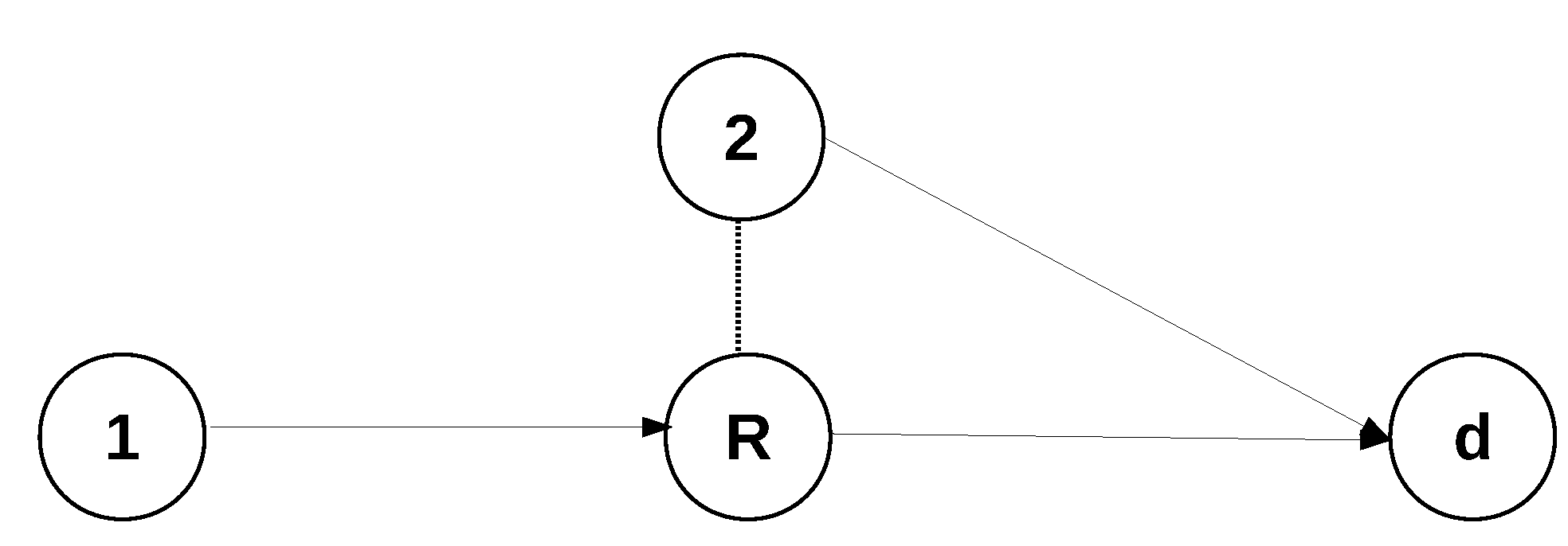
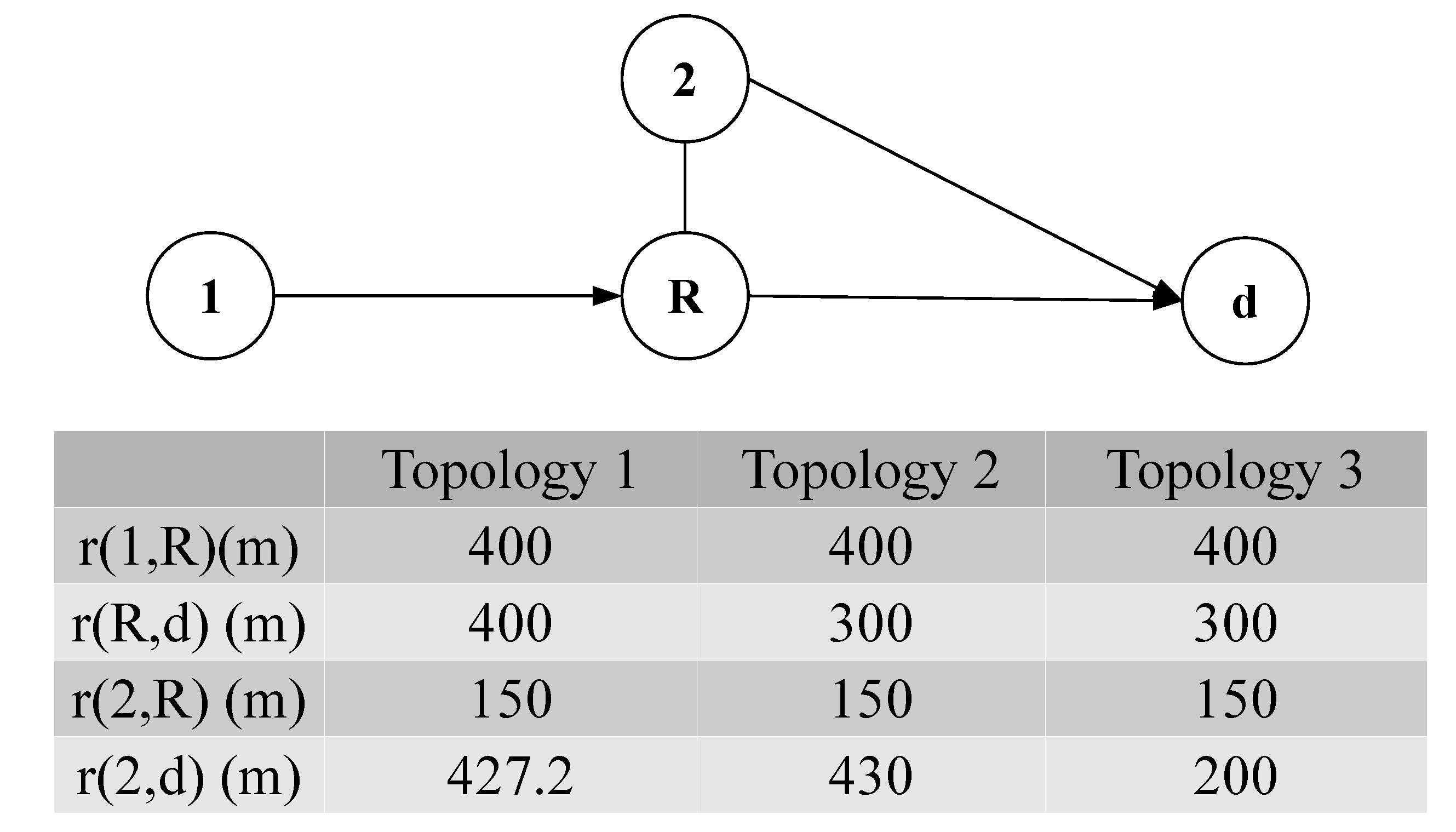
19]. For that reason, three different topologies are explored, based on the one presented in Figure 2. Different topology instances are derived by fixing the distances between pairs of nodes. The corresponding distance values employed are summarized in the table incorporated in the same figure. For all three topologies, two unicast flows are assumed, sourced at nodes, 1 and 2, respectively. Flow f 1 , is forwarded to d, through path 1 R d , while flow f 2 , through 2 d . Assuming such a traffic scenario, in topology 1 presented in Figure 2, transmissions along link ( 1 , R ) experience interference from node 2. If similar SINR threshold ( γ ) values, for all transmitters, are further assumed, then the received signal on R from 2, constituting the interference, is received with higher power compared to the signal received from 1. In a similar manner, in topologies 1 and 2, transmissions along link ( 2 , d ) experience interference from R. The signal constituting interference from R is received with higher power at d than the signal carrying data packets sent from 2.
Based on these remarks, for each topology in Figure 2, we consider different interference handling approaches. For topologies 1 and 2, three different approaches for handling interference are explored. In the first one, interference at nodes R, d is treated as noise. In the second approach, SIC is applied on R, as described in Section 3. In the third one, destination d, first tries to decode the message from R, remove its contribution (interference) to the received signal, and then decode the message from 2. Finally, as far as topology 3, depicted in Figure 2, is concerned, three approaches are also explored. The first two approaches are the same with topologies 1 and 2. In the third one, however, where the destination resides closer to transmitting node 2 instead of R, d first tries to decode the message received from 2 (interference), remove its contribution to the received signal, and then decode the message from node R. For the rest of the section, we will also use the term successive interference cancelation to describe how interference is handled at destination d. To distinguish among the different approaches discussed above for handling interference, they are labelled after: IAN, SIC(R), SIC(R,d), with SIC(R,d) denoting that SIC is applied at both R and d.
As far as allocation of flow (data rates) on different paths is concerned, three different schemes are explored. The first scheme is TOFRA (presented in Section 3). Full MultiPath (FMP) assigns one packet per slot on each path. Finally, the third scheme explored employs only a single path (best path) to forward traffic to the destination. Based on how best path is identified, we explore two variants: in the first one, denoted as BP e 2 e , best path is considered as the one exhibiting the highest end-to-end success probability, and is identified through: r ^ k : arg max r k ( i , j ) r k p i / i j . In the second variant, denoted as BP w b , best path is defined as the one that has the widest bottleneck link, which can be formulated as identifying path r ^ k : arg max k min ( i , j ) r k ) p i / i j . In the first two topologies explored, BP w b utilizes path 1 R d to the destination, while in the third one, 2 d . BP e 2 e on the other hand, deploys path 2 d , for all three topologies explored. Applying SIC for the cases of the best-path variants and the topologies presented in Figure 2 is meaningless since, when path 2 d is used, destination d receives no interference, while in the case of 1 R d , the interference received at d, from 1, is insignificant due to the large distance between them. For both aforementioned best-path variants, the flow assigned on the utilized single path is calculated by solving a single-path version of the optimization problem (P2), presented in Section 3, through the simulated annealing technique.
Different simulation scenarios are generated as follows: for each topology presented in Figure 2, one of the aforementioned flow allocation schemes is employed. For each flow allocation scheme, three variants are simulated based on how interference is handled at each receiving node. The variant denoted by FMP-IAN for example, assigns one packet per slot on each path, while interference is treated as noise at each receiver. For FMP-SIC(R), SIC is assumed at receiving node R. To capture the effect of interference on success probability, four different SINR threshold values are employed: 0.5 , 1.0 , 1.5 , and 2.0 . In each simulation scenario, flows carrying constant bit rate, UDP traffic, are generated while the simulation period is 20,000 slots. Queues for flow originators are kept backlogged for the whole simulation period. For the relay node present in Figure 2, the queue may become empty during a slot, i.e, queues for relay nodes are not assumed to be saturated in all the simulated scenarios.
In the first part of the evaluation process, we explore whether the proposed model accurately captures the average aggregate flow throughput (AAT) observed in the simulation results. Table 3, Table 4 and Table 5, summarize the flow rates assigned on each path, along with the corresponding value for AAT achieved by TOFRA, derived from both the numerical and the simulation results. Recall that flow rates assigned on each path are identified by sources, by solving a topology specific instance of the flow allocation optimization problem presented in Section 3. The path loss exponent assumed for deriving numerical results is 3.0 and link distances are those presented in Figure 2.
The average deviation between the AAT derived from the model described in Section 3 and the one observed in the simulated results, is 1.42 % , over all topologies, γ values, and TOFRA variants employed. There are several reasons for this deviation. The main one is related to the assumption of the model, for AAT, concerning saturated queues at the relay nodes. In our analysis, it is assumed that whenever a relay node attempts to transmit a packet, there is always one available in its queue. In the simulated scenarios, however, a relay node’s queue may be empty at a specific slot. In this way, the considered model for the AAT overestimates the interference experienced by any link in the simulated scenarios and thus, underestimates the average throughput achieved over that link. Due to the assumption concerning saturated queues at the relay nodes, it also overestimates the collision probability at each relay node, due to concurrent packet transmission and reception events. At the end of this section, we also discuss how this underestimation of a link’s average throughput may also affect queueing delay. Apart from that, in the analysis presented in Section 3, a packet is not assumed to be dropped after a larger number of failed retransmissions. In the simulation parameters presented in Table 6, however, a maximum retransmit threshold equal to 3 is adopted. This suggests that, after three failed transmissions, a specific packet is dropped. This may result in lower throughput for the link over which that packet is retransmitted, but will also result in reduced interference imposed on neighbouring links. Finally, in the analysis, we have assumed that whenever a packet is transmitted, it is a packet carrying data. In the simulated scenarios, however, all nodes either perform periodic emission of routing protocol’s control messages or forwarded specific topology control packets. This means that specific slots are spent carrying routing protocol’s control messages, instead of data packets, resulting in our analysis overestimating the AAT observed in the simulated results.
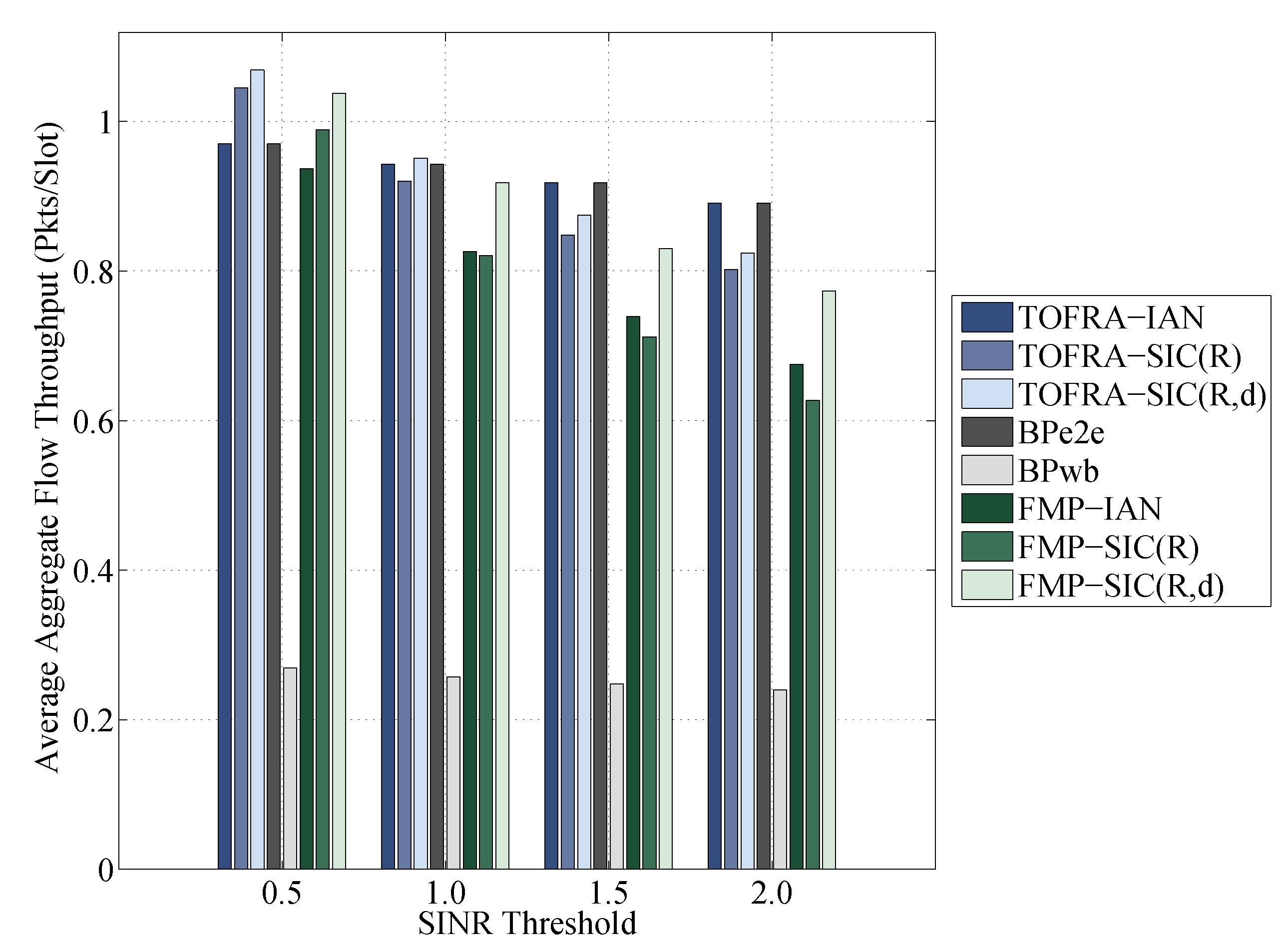
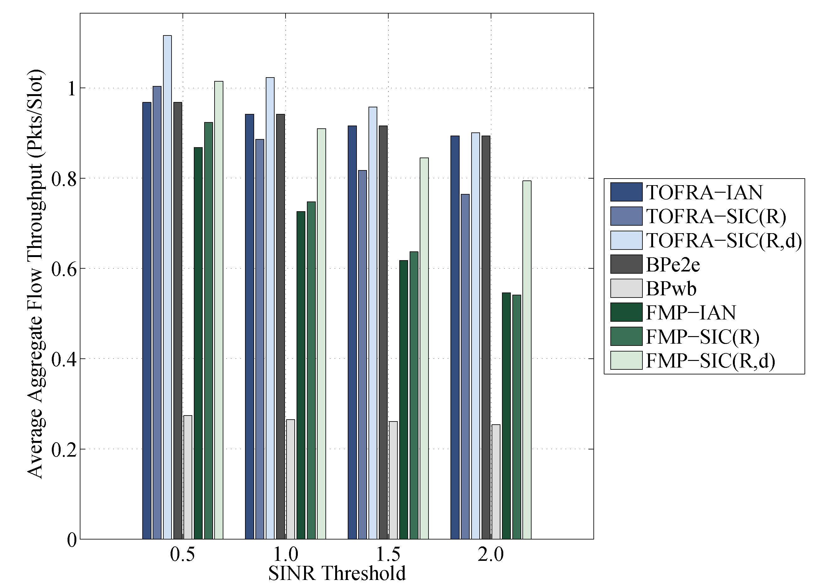
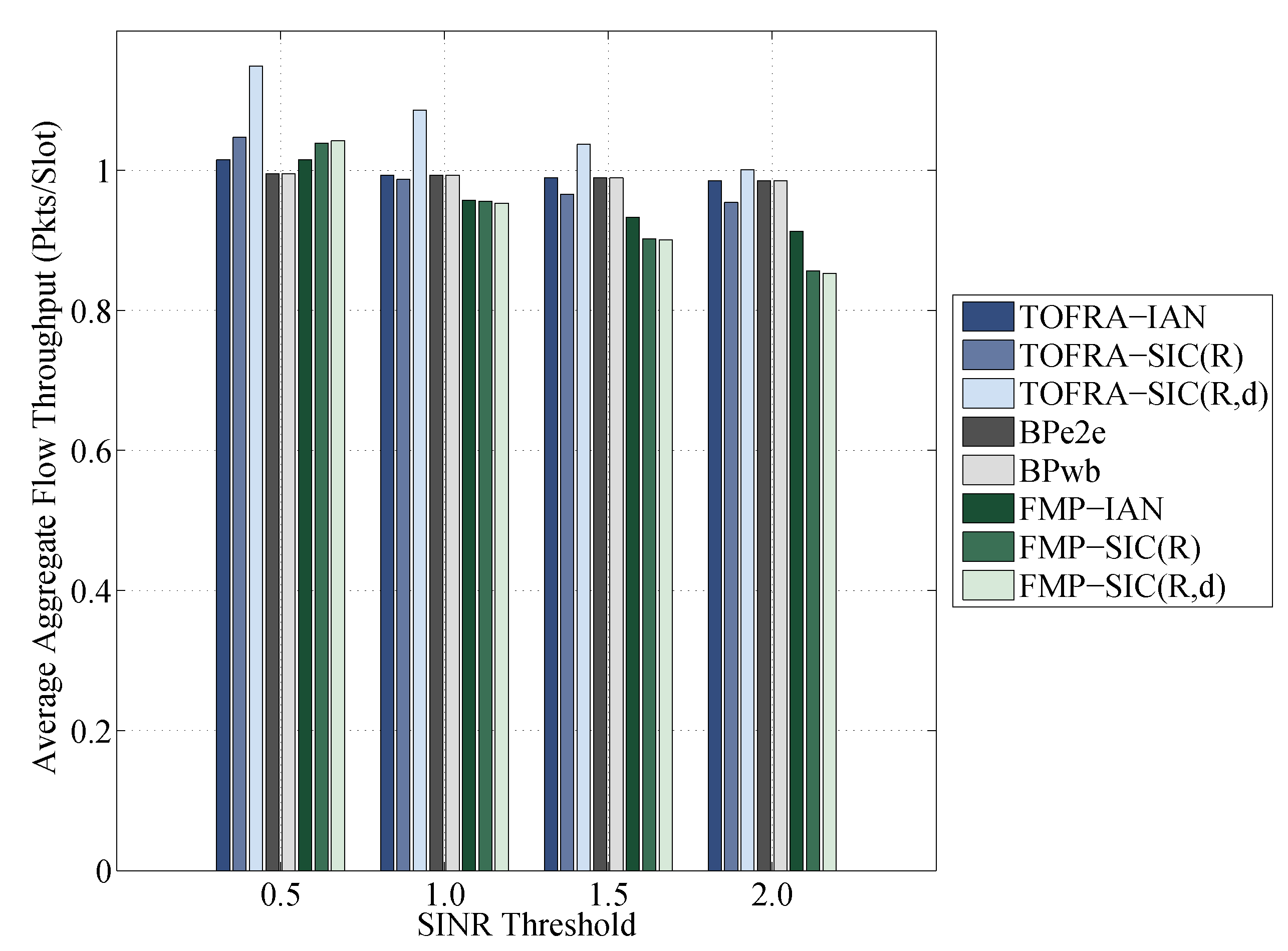
In the second part of the evaluation process, we explore the gain in terms of throughput that can be achieved by employing SIC, instead of treating interference as noise (IAN). More precisely, we explore the AAT achieved by the aforementioned flow allocation schemes, when different approaches for handling interference are followed (discussed above). Figure 3, Figure 4 and Figure 5 present the corresponding AAT values for the three topologies summarized in Figure 2.
Table 3, Table 4 and Table 5 show that applying SIC instead of IAN, at both receiving nodes R, d, proves gainful in terms of AAT, when γ = 0.5. For the case of the TOFRA flow allocation scheme, the gain is 10.2 % , 15.2 % , and 13.2 % , respectively, for the three topologies considered. It should also be noted that the gain in terms of throughput, for SIC, is less significant when it is applied only to receiver R. For γ = 0.5, employing SIC at R, instead of IAN, results in 7.7 % , 3.7 % , and 3.1 % higher AAT, for the three topologies explored. Applying SIC on R, increases the success probability on link ( 1 , R ) , from 9.3 % to 95.1 % , for γ = 0.5 and from 2.3 % to 81.5 % for γ = 2.0. Consequently, transmitter 1 will manage to deliver a larger portion of its traffic to R, when SIC is employed at R, instead of IAN, which will also result in an increased number of packets transmitted from R to d. This will have a negative effect on the average throughput of link ( 2 , d ) since it will experience increased interference. Focusing on the first topology presented in Figure 2, γ = 0.5 and the TOFRA flow allocation scheme we observe the following; when interference is treated as noise at all receivers, the fraction of data packets transmitted over ( 2 , d ) that are retransmitted due to noise, signal attenuation, interference, and fading, is 2.7 % . In the scenario where SIC is employed at R, the corresponding fraction of retransmitted packets increases to 14.1 % . This shows that improving the success probability at a relay node by applying SIC, will also increase the interference imposed on its next hop. Consequently, the number of packets that are retransmitted will increase, limiting the gain in terms of AAT. As Table 3, Table 4 and Table 5 also show, for higher γ values, applying SIC instead of IAN, for the case of TOFRA, either offers insignificant gain or results in lower average aggregate throughput. As already discussed, applying SIC at R significantly increases the success probability on link ( 1 , R ) , with TOFRA also increasing the amount of flow assigned on path 1 R d . However, if the increased interference on link ( 2 , d ) is not compensated by the gain of utilizing path 1 R d , the average aggregate flow throughput (AAT) observed, may be lower compared to the case where IAN is applied at each receiver.
As far as the relation between interfering links asymmetry and gain in terms of throughput of SIC over IAN is concerned, the following remark is also interesting. As already discussed above, the success probability of link ( 1 , R ) increases from 9.3 % to 95.1 % , for γ = 0.5, when SIC is employed at R, instead of IAN. Accordingly, in topology 1 for example, the success probability of link ( 2 , d ) increases from 60.4 % to 66.7 % for γ = 0.5, when SIC is employed at d, instead of IAN. This increase in the success probability is significantly lower than the corresponding one for link ( 1 , R ) . The reason for this is the different asymmetry between interfering links for the two receivers. As Figure 2 also shows, the distance of interfering node 2 from R is much smaller than the distance between 1 and R. The distances, however, of nodes 2 and R, from d, are very similar. A notable effect of combining SIC with the TOFRA flow allocation scheme is the utilization of paths that were assigned zero flow when IAN was applied at receiving nodes. As Table 3, Table 4 and Table 5 show, the utilization of path 1 R d becomes non-zero for all topologies and γ values considered when SIC is employed.
In the third part of the evaluation process, the proposed scheme is compared with FMP and best path-based flow allocation schemes, both in terms of throughput and delay. Variants of the TOFRA scheme achieve higher AAT than the corresponding full multipath (FMP) variants, for all topologies and γ values employed. The main reason for this is that FMP assigns one packet per slot on each path in an interference unaware manner, resulting in a higher fraction of data packets retransmitted due to interference. This performance gap becomes even more profound when large SINR threshold values are assumed where the success probability of all links is decreased. Considering topology 3, with γ = 0.5 for example, TOFRA-SIC( R , d ) achieves 10.2 % higher AAT than the corresponding FMP variant (FMP-SIC( R , d )). Compared to BP e 2 e , TOFRA-IAN achieves the same AAT, for almost all scenarios explored, since they both utilize at full rate path 2 d . The only exception to this is the scenario based on topology 3, where γ = 0.5. In this scenario, the corresponding TOFRA variant also utilizes path 1 R d . When TOFRA, however, is combined with SIC, at both R and d and a low γ is employed, it achieves higher AAT. In topology 3 for example, when a γ value equal to 0.5 is employed, TOFRA-SIC( R , d ) achieves 15.4 % higher AAT than BP e 2 e . It should be noted, however, that the prospect of higher throughput for TOFRA is limited by the number of paths available. In [24,26] where several paths are employed in parallel, TOFRA outperforms the corresponding best-path variant. Finally, the best-path variant, which selects the path with the widest bottleneck link, in terms of success probability (BP w b ), utilizes path 1 R d for topologies 1 and 2, and 2 d for topology 3. However, as Table 3, Table 4 and Table 5 show, TOFRA assigns zero flow on path 1 R d for most scenarios explored, when interference is treated as noise. This shows that utilizing this path in parallel with 2 d would result in lower AAT. As also shown in Figure 3, Figure 4 and Figure 5, BP w b achieves the lowest AAT among all schemes, for topologies 1 and 2, and performs the same with BP e 2 e for topology 3. To summarize, simulation results presented in Figure 3, Figure 4 and Figure 5 reveal that TOFRA, when combined with SIC at both the relay and the destination, achieves the highest AAT than all flow allocation schemes in almost all topologies and γ values considered. The only exception is the simulation scenarios derived from Topology 1 and γ values 1.5 and 2.0 . In these scenarios, the variant of TOFRA that treats interference as noise achieves the highest AAT along with B P e 2 e .
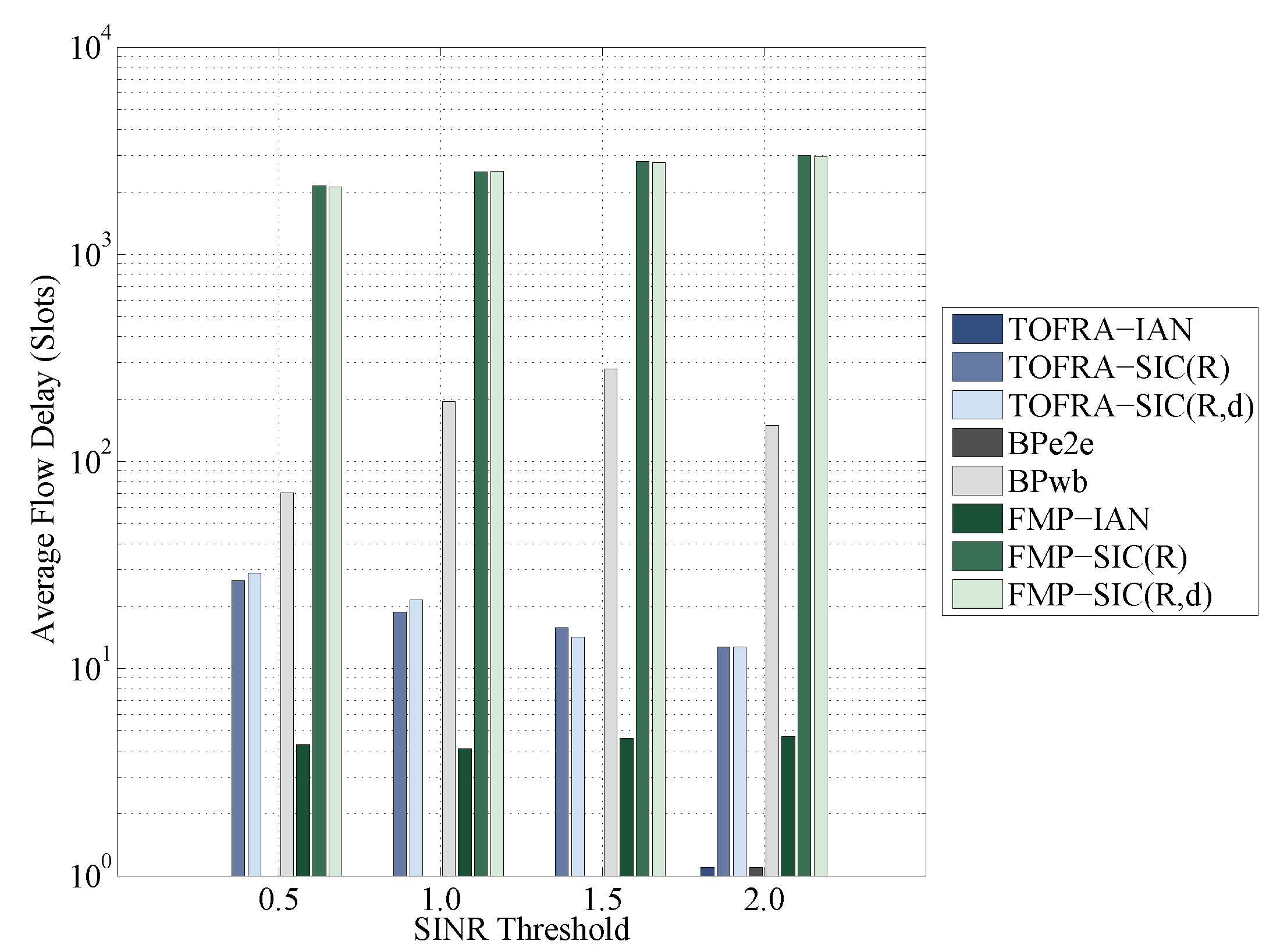
In this part of this section, the aforementioned flow allocation schemes are also compared in terms of delay. More precisely, the average flow delay, measured in slots, for each scheme is estimated. Before discussing simulation results, the following definitions are necessary: for each flow, end-to-end flow delay will be used to denote the average per-packet end-to-end delay, for all packets forwarded by that flow. End-to-end delay for a packet is the interval between that packet’s first transmission attempt at the source of the flow and the time when the packet is successfully received at the destination of the corresponding flow. For the rest of the section, average flow delay will be referred to as flow delay.
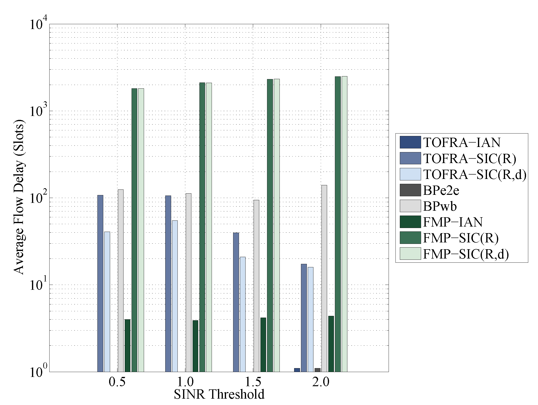
Figure 6, Figure 7 and Figure 8 present average flow delay for the three topologies described in Figure 2 and the four SINR threshold values considered. For the rest of the section, end-to-end flow delay will be referred to as flow delay.
As these figures show, for all three topologies explored, TOFRA-IAN achieves the same delay with BP e 2 e , for all γ values considered. The only exception to this is the simulated scenario based on topology 3, with γ = 0.5. In this scenario, TOFRA-IAN also assigns flow on path 1 R d . The flow assigned on path 1 R d is also increased in the case where TOFRA is combined with SIC. As Table 3 for example shows, for the second topology and γ = 0.5, TOFRA assigns 0.350 packets per slot on path 1 R d , when SIC is applied at both R and d. Consequently, a larger number of packets will experience queueing delay at R and also increased retransmissions due to inter-path interference. The effect of queueing delay on flow delay is extensively discussed in the rest of the section. This effect is also validated if BP w b is considered for topologies 1 and 2. In these topologies, BP w b forwards all packets through path 1 R d . Figure 6, Figure 7 and Figure 8 show that it experiences significantly higher flow delay than all other schemes with the exception of full multipath variants FMP-SIC(R), FIM-SIC( R , d ). The second reason behind the increased delay of TOFRA, when combined with SIC, is related to the accuracy with which the model presented in Section 3 captures the average throughput of a link and is discussed in the next paragraph.
To validate the effect of queueing delay on flow delay, the throughput ratio for a relay, along with average queue length are employed. For the case of relay node R, in Figure 2 for example, throughput ratio is defined as: T ¯ ( 1 , R ) / T ¯ ( R , d ) . A value for that ratio larger than one would suggest queueing at the relay, since packets arrive at a rate faster than the rate with which they can be serviced (delivered to d). This results in an unstable queue at the relay node and consequently in packets experiencing unbounded delay. A value for that ratio that is one, would imply a sub-stable queue at R. In this case, packets may experience an increased queueing delay. Additionally, the average queue length for each node, especially for the relays, is calculated from simulated results.
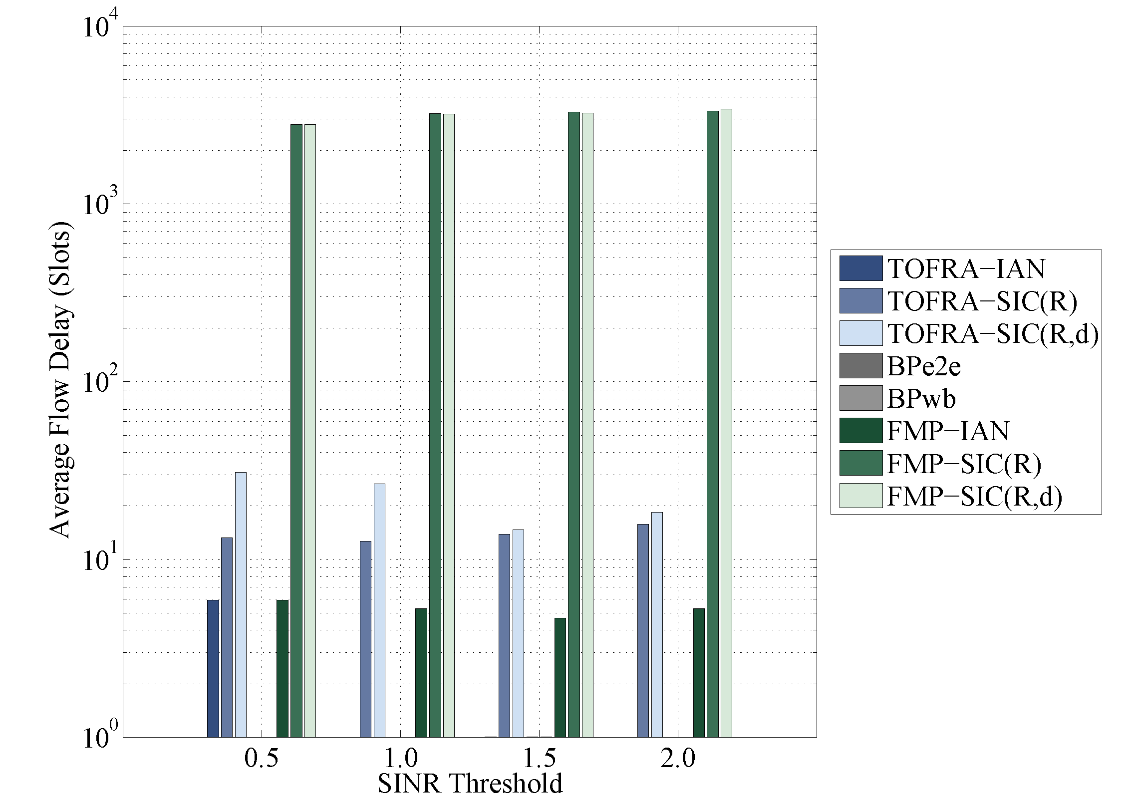
Figure 6, Figure 7 and Figure 8 also show that, for all topologies and γ values explored, FMP-IAN achieves significantly lower flow delay than TOFRA variants that employ SIC, although FMP is expected to experience more failed packets due to increased inter-path interference. In order to explore this delay gap between FMP and TOFRA variants, topology 2, with γ = 0.5, is used as an example. Moreover, we focus on FMP-IAN and TOFRA-SIC( R , d ) variants. As the simulation results show, FMP-IAN indeed experiences a larger number of failed transmission due to noise, signal attenuation, interference, and fading. For link ( 0 , 1 ) , this ratio is 81.0 % for FMP-IAN and 3.6 % for TOFRA-SIC( R , d ). As far as path 1 R d is concerned, it is also interesting to note that FMP-IAN manages to deliver to R, only 8.3 % of the packets sent over link ( 1 , R ) , while the corresponding value for TOFRA-SIC( R , d ) is 68.6 % . Taking into account these ratios, TOFRA-SIC( R , d ) is expected to experience higher queueing delay than FMP-IAN. Indeed, the average queue length for relay node 1 is 0.09 packets, for the case of FMP-IAN, and 17.0 packets when TOFRA-SIC( R , d ) is employed.
Comparing different TOFRA variants in terms of average flow delay shows that when SIC is applied, instead of IAN, average flow delay exhibits a significant increase. As Table 3, Table 4 and Table 5 show, when TOFRA is combined with SIC, maximum AAT is achieved by utilizing path 1 R d in parallel with 2 d , for all topologies explored. The gap in terms of delay may imply that TOFRA variants that employ SIC experience increased queueing delay. To validate this, the simulation scenario based on topology 2 with γ = 0.5, is used as an example. First, the throughput ratio for relay node R is estimated, for the two TOFRA variants that employ SIC, from simulation results. The value of this ratio is 1.02 , and 1.01 , respectively, for the two considered variants, suggesting that the queue at R becomes unstable. However, as already discussed in the first part of the evaluation process, the model employed for the average aggregate flow throughput, may underestimate the actual average throughput of a link observed in the simulation scenarios. In this way, the average throughput of a specific link may be higher than the average throughput of a subsequent link which results in an unstable queue at the relay. The second reason is that SIC improves the success probability of link ( 1 , R ) and, thus, increases the number of packets that are successfully delivered to R, when compared to TOFRA-IAN, resulting in a larger average queue size.
For all topologies and γ values explored, when full multipath (FMP) is combined with SIC, either at R, or both at R and d, it experiences by far higher average flow delay than all other flow allocation schemes discussed. For topology 1, in Figure 2 and γ = 0.5 for example, the flow delay observed in the simulation results, for FMP-SIC(R) and FMP-SIC( R , d ), is 2133.9 and 2111.3 slots, respectively. However, this is expected, since FMP assigns traffic on paths in an interference-unaware manner, experiencing a large number of failed packets due to increased interference. Secondly, it does not adjust the flow assigned on a path based on the one that can be serviced by its bottleneck link, resulting thus, in unstable queues at the relay nodes. For the case of topology 1 with γ = 0.5 mentioned above, the throughput ratio at R for FMP-SIC(R) and FMP-SIC( R , d ) is 3.680 and 3.658 , respectively.
As a brief overview of the results concerning flow delay, when TOFRA is combined with SIC, either at the relay or at both the relay and the destination, the delay achieved is significantly worse than TOFRA variant that treats interference as noise (TOFRA-IAN). The reason is that in all simulated scenarios, TOFRA-IAN forwards all traffic to the destination through a single hop path 2 d . Consequently, packets do not experience a queueing delay at relay node R as in the case of TOFRA-SIC(R) and TOFRA-SIC( R , d ).
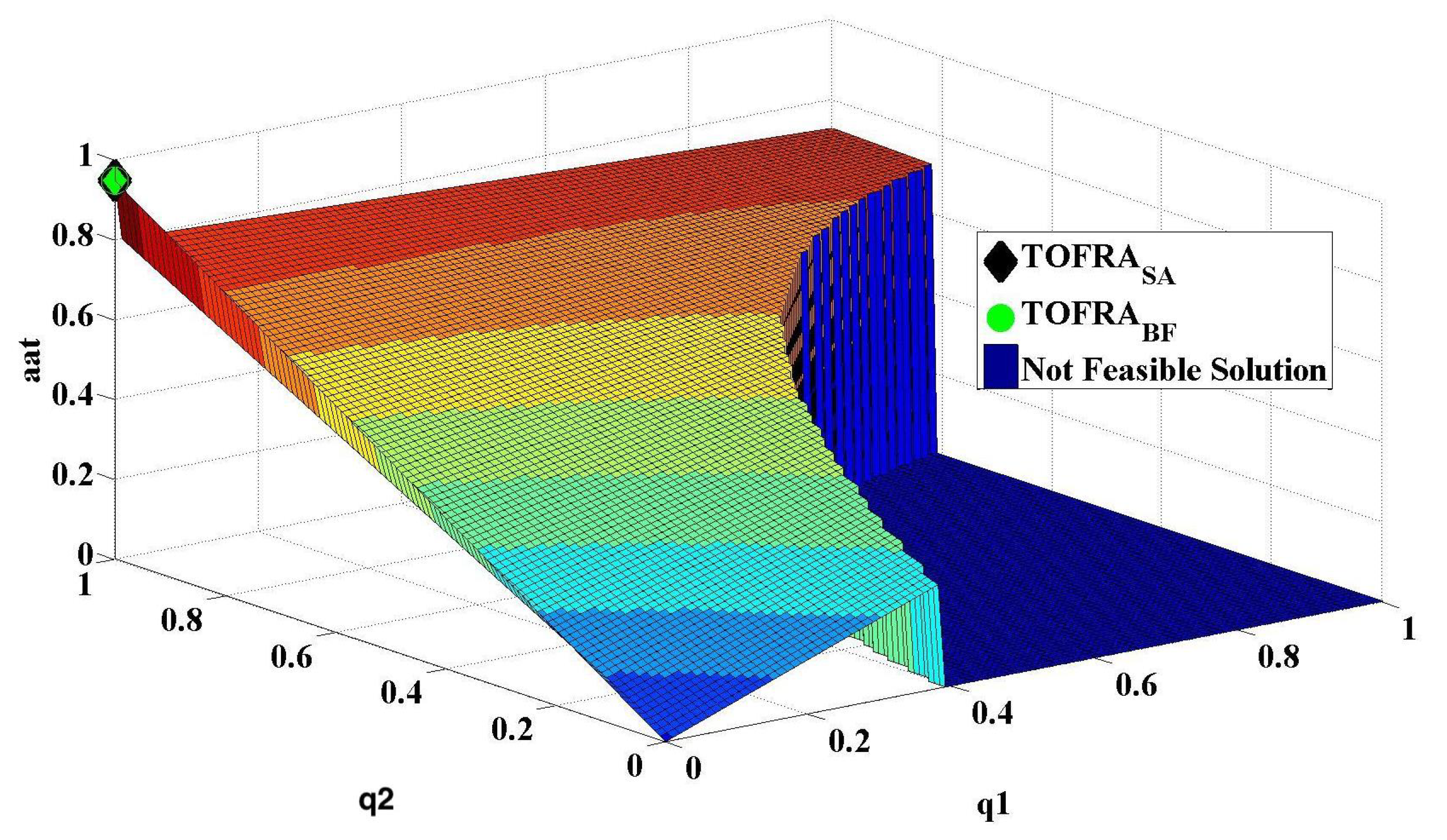
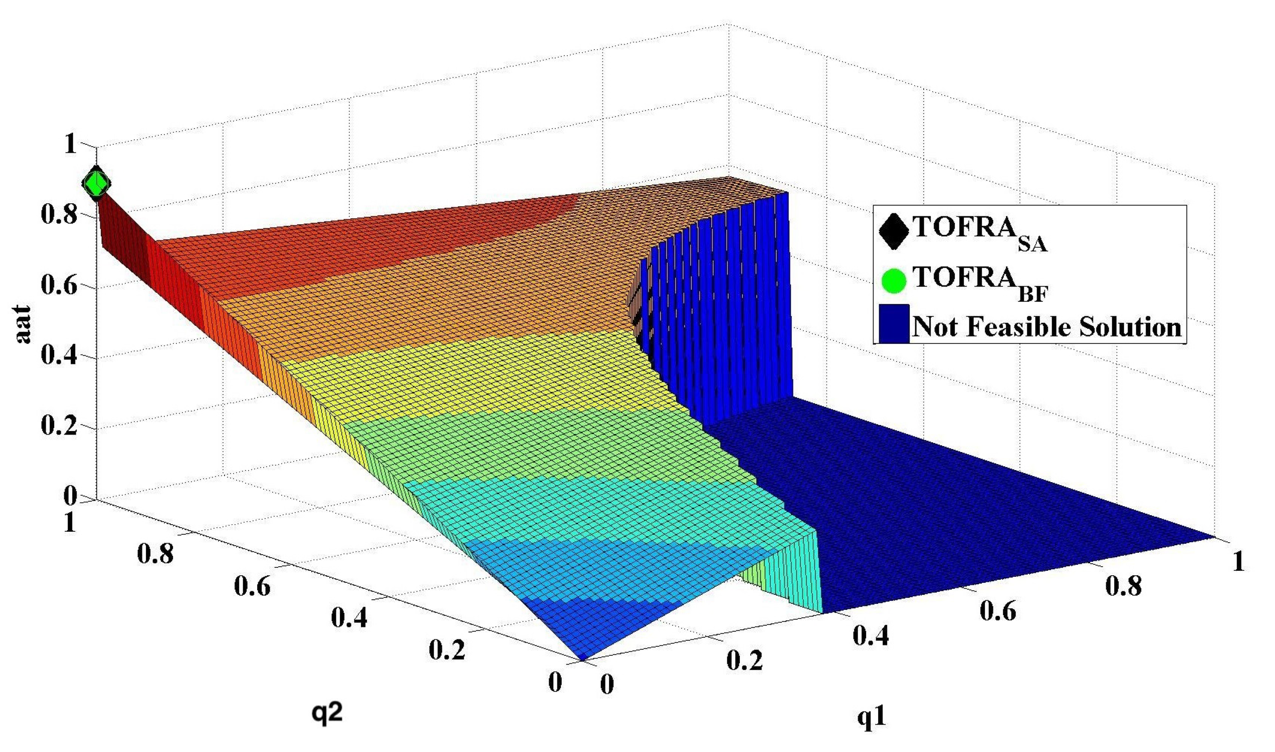
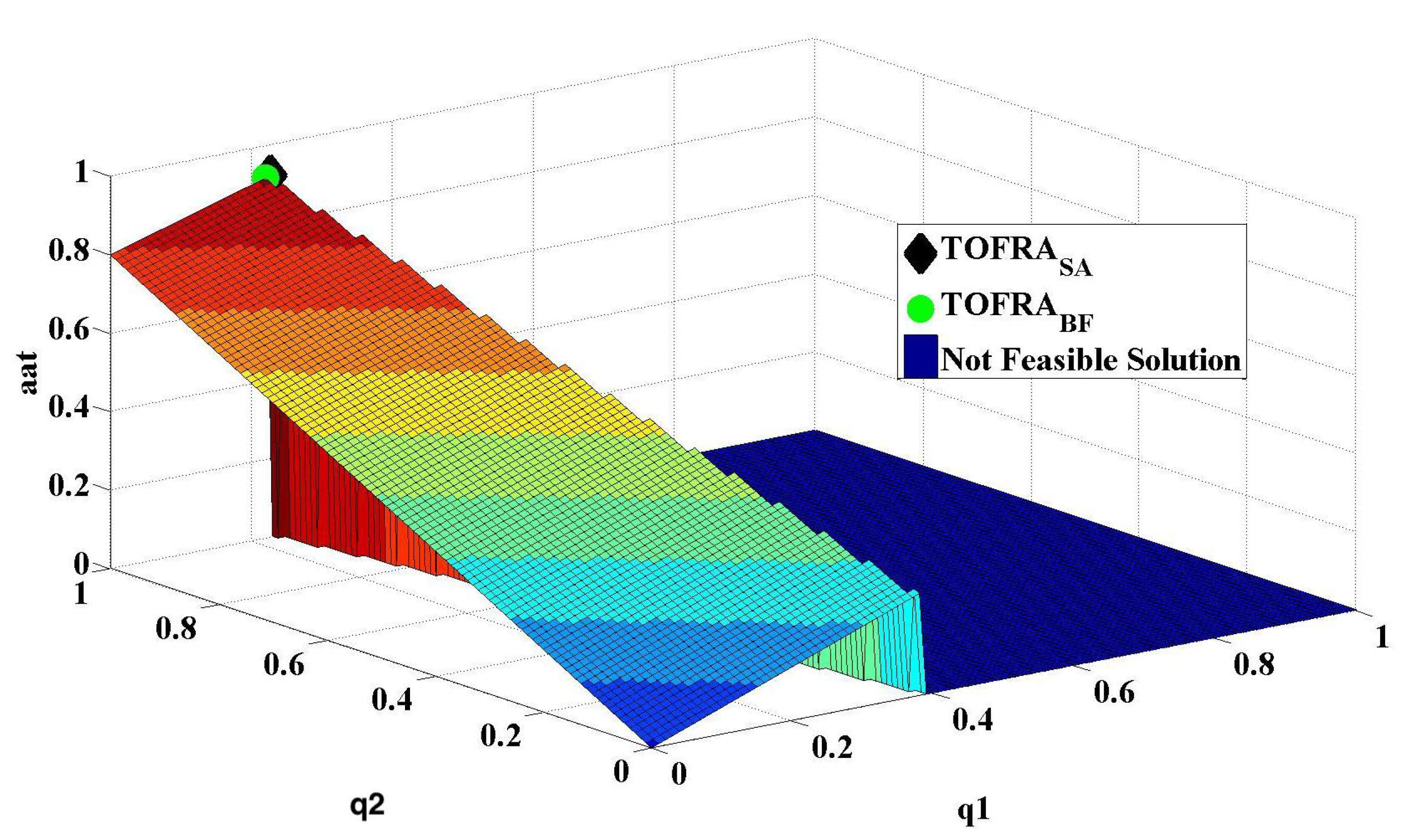
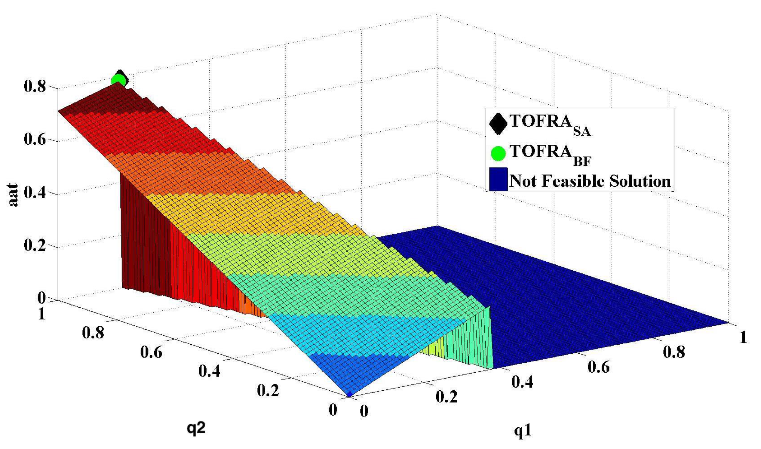
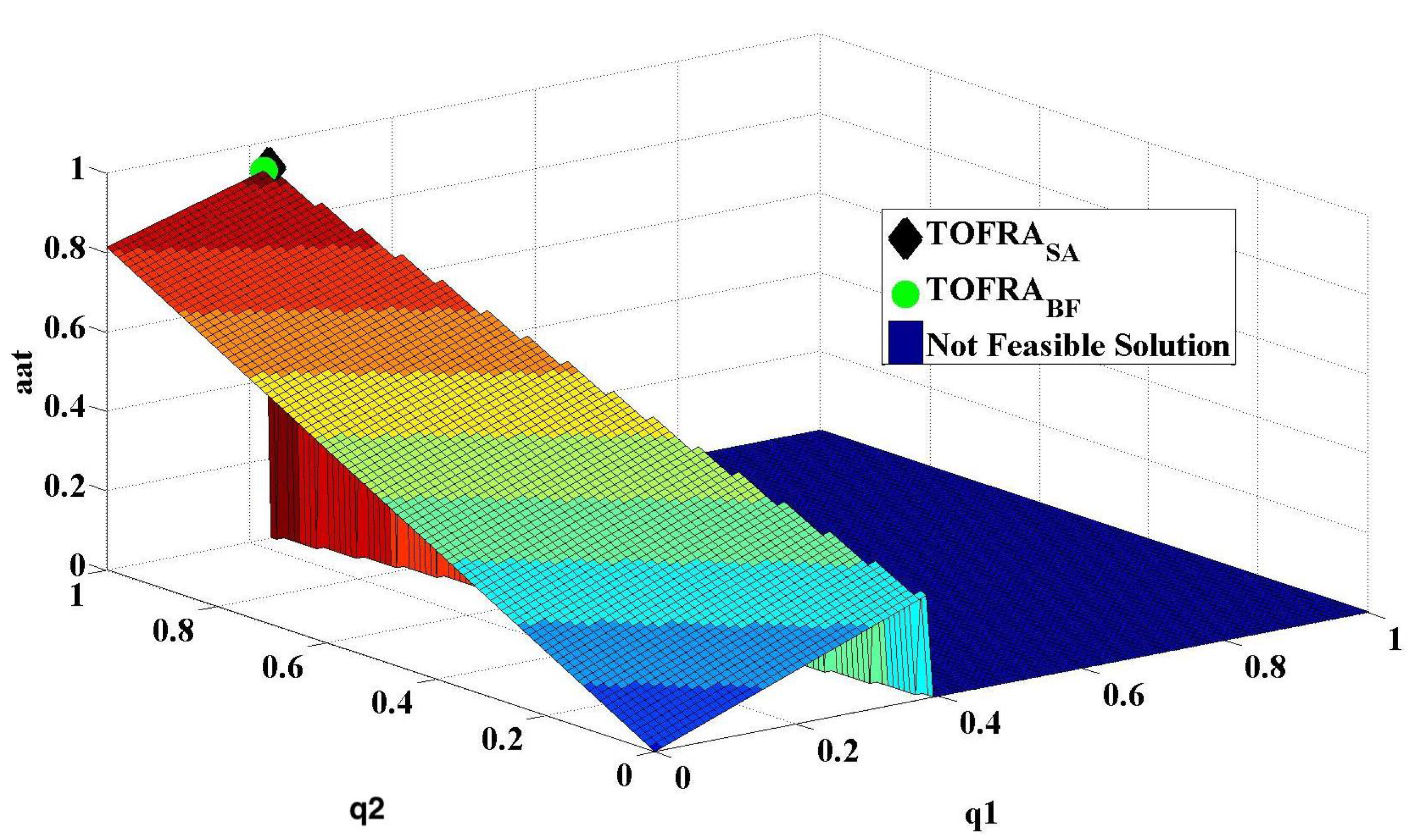
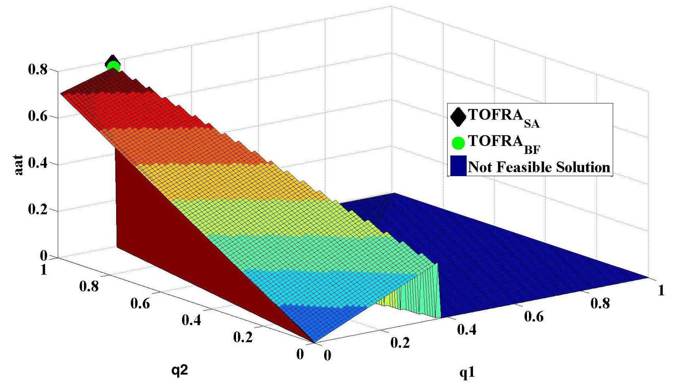
In the final part of the evaluation process, we explore the accuracy with which the simulated annealing method approaches the flow rates that achieve the globally maximum AAT. Towards this direction, a brute force search algorithm is implemented. The brute force algorithm explores all different combinations, of values for the optimization problem’s variables. Different values of a specific variable are generated using a specific step size with values for that variable ranging in [ 0 , 1 ] . Our goal is to compare the solution to the flow allocation problem identified by the simulated annealing and the brute force algorithm. An insignificant gap between the two solution points would suggest that simulated annealing has accurately managed to identify the flow rates that achieve the highest AAT among all feasible solution points. To assist visual inspection of the gap between the solution identified by the simulated annealing and brute force algorithms, we plot the corresponding solutions for a subset of the simulation scenarios explored in this section. More precisely, we focus on Topology 1 of Figure 2, SINR threshold values 1.0 , and 2.0 and all three TOFRA variants. Figure 9, Figure 10, Figure 11, Figure 12, Figure 13 and Figure 14 compare the average aggregate throughput (AAT) achieved by TOFRA when flow rates assigned on each path are estimated through simulated annealing (TOFRA S A ) or through the brute force search algorithm using a step of 0.01 (TOFRA B F ). The flow rates that need to be fixed so as to maximize AAT are q 1 and q 2 , respectively. Moreover, two different SINR threshold ( γ ) values are considered, 1.0 , and 2.0 . In the aforementioned figures, values for the AAT, measured in packets per slot, are presented on the vertical, z-axis. Values for the AAT that are equal to 0.0 correspond to a combination of flow rates that do not constitute a feasible solution to the flow allocation optimization problem. This suggests that the bounded delay constraint (also discussed in Section 3) is violated. As these figures show, the solution identified by simulated annealing lies very close to the pair of q 1 and q 2 values, that achieve the highest AAT according to the BF algorithm.

6. Conclusions and Future Extensions

In this work, we explore the gain that can be achieved by jointly allocating flow on multiple paths and employing successive interference cancelation (SIC) for random access wireless mesh networks. More precisely, we explore a distributed flow allocation scheme aimed at maximizing average aggregate flow throughput, while also providing bounded delay, when SIC is employed. The flow allocation scheme discussed achieves up to 15.2 % higher AAT when combined with SIC, instead of treating interference as noise (IAN), for an SINR threshold ( γ ) value equal to 0.5 . For larger γ values, this improvement either becomes negligible, or lower AAT is achieved for the topologies considered. This is because the increased interference caused by links whose success probability is significantly increased with SIC is not compensated by the gain in terms of throughput. Moreover, the improvement in terms of throughput by employing SIC instead of IAN increases with the asymmetry among interfering links.
Future extensions of this work will include the deployment of SIC jointly with TOFRA on larger topologies. The proposed framework can be applied in large topologies, as long as the link success probabilities can be calculated for different interference handling approaches, such as SIC. However, considering SIC in such topologies, when there is more than one interfering node to decode, has its challenges. Furthermore, it would be of interest to study the case where a receiver works in a hybrid manner by treating interference as noise or applying SIC based on the network conditions.

Author Contributions

The first and second author have contributed equally. The third author has proofread and supervised the work. All authors have read and agreed to the published version of the manuscript.

Funding

This research received no external funding.

Institutional Review Board Statement

Not applicable.

Informed Consent Statement

Not applicable.

Data Availability Statement

Not applicable.

Acknowledgments

The authors would like to thank the Editor Marios Gatzianas for improving the quality of this work with his suggestions.

Conflicts of Interest

The authors declare no conflict of interest.

References

  1. Le, L. Multipath Routing Design for Wireless Mesh Networks. In Proceedings of the Global Telecommunications Conference (GLOBECOM 2011), Houston, TX, USA, 5–9 December 2011; pp. 1–6. [Google Scholar] [CrossRef]
  2. Alicherry, M.; Bhatia, R.; Li, L.E. Joint Channel Assignment and Routing for Throughput Optimization in Multiradio Wireless Mesh Networks. Sel. Areas Commun. IEEE J. 2006, 24, 1960–1971. [Google Scholar] [CrossRef]
  3. Middleton, G.; Aazhang, B.; Lilleberg, J. Efficient Resource Allocation and Interference Management for Streaming Multiflow Wireless Networks. In Proceedings of the Communications (ICC), 2010 IEEE International Conference, Cape Town, South Africa, 23–27 May 2010; pp. 1–5. [Google Scholar] [CrossRef]
  4. Middleton, G.; Aazhang, B.; Lilleberg, J. A Flexible Framework for Polynomial-Time Resource Allocation in Streaming Multiflow Wireless Networks. Wirel. Commun. IEEE Trans. 2012, 11, 952–963. [Google Scholar] [CrossRef]
  5. Gao, Q.; Zhang, J.; Hanly, S. Cross-layer rate control in wireless networks with lossy links: Leaky-pipe flow, effective network utility maximization and hop-by-hop algorithms. Wirel. Commun. IEEE Trans. 2009, 8, 3068–3076. [Google Scholar] [CrossRef]
  6. Lin, X.; Shroff, N. Joint rate control and scheduling in multihop wireless networks. In Proceedings of the 2004 43rd IEEE Conference on Decision and Control (CDC) (IEEE Cat. No.04CH37601), Nassau, Bahamas, 14–17 December 2004; Volume 2, pp. 1484–1489. [Google Scholar] [CrossRef]
  7. Akyol, U.; Andrews, M.; Gupta, P.; Hobby, J.; Saniee, I.; Stolyar, A. Joint Scheduling and Congestion Control in Mobile Ad-Hoc Networks. In Proceedings of the INFOCOM 2008, the 27th Conference on Computer Communications, Phoenix, AZ, USA, 13–18 April 2008; pp. 619–627. [Google Scholar] [CrossRef]
  8. Chen, L.; Low, S.; Chiang, M.; Doyle, J. Cross-Layer Congestion Control, Routing and Scheduling Design in Ad Hoc Wireless Networks. In Proceedings of the INFOCOM 2006, 25th IEEE International Conference on Computer Communications, Barcelona, Spain, 23–29 April 2006; pp. 1–13. [Google Scholar] [CrossRef] [Green Version]
  9. Yu, Y.; Giannakis, G. Cross-layer congestion and contention control for wireless ad hoc networks. Wirel. Commun. IEEE Trans. 2008, 7, 37–42. [Google Scholar] [CrossRef] [Green Version]
  10. Wang, X.; Kar, K. Cross-layer rate optimization for proportional fairness in multihop wireless networks with random access. Sel. Areas Commun. IEEE J. 2006, 24, 1548–1559. [Google Scholar] [CrossRef] [Green Version]
  11. Uddin, M.; Rosenberg, C.; Zhuang, W.; Girard, A. Joint Configuration of Routing and Medium Access Parameters in Wireless Networks. In Proceedings of the Global Telecommunications Conference, 2009, GLOBECOM 2009, Honolulu, HI, USA, 30 November–4 December 2009; pp. 1–8. [Google Scholar] [CrossRef]
  12. Weber, S.P.; Andrews, J.; Yang, X.; de Veciana, G. Transmission Capacity of Wireless Ad Hoc Networks With Successive Interference Cancellation. Inf. Theory IEEE Trans. 2007, 53, 2799–2814. [Google Scholar] [CrossRef]
  13. Verdu, S. Multiuser Detection, 1st ed.; Cambridge University Press: New York, NY, USA, 1998. [Google Scholar]
  14. Toumpis, S.; Goldsmith, A. Capacity regions for wireless ad hoc networks. Wirel. Commun. IEEE Trans. 2003, 2, 736–748. [Google Scholar] [CrossRef]
  15. Yuan, D.; Angelakis, V.; Chen, L.; Karipidis, E.; Larsson, E. On Optimal Link Activation With Interference Cancelation in Wireless Networking. Veh. Technol. IEEE Trans. 2013, 62, 939–945. [Google Scholar] [CrossRef] [Green Version]
  16. Mitran, P.; Rosenberg, C.; Shabdanov, S. Throughput optimization in wireless multihop networks with Successive Interference Cancellation. In Proceedings of the Wireless Telecommunications Symposium (WTS), 2011, New York, NY, USA, 13–15 April 2011; pp. 1–7. [Google Scholar] [CrossRef] [Green Version]
  17. Zhang, X.; Haenggi, M. The Performance of Successive Interference Cancellation in Random Wireless Networks. IEEE Trans. Inf. Theory 2014, 60, 6368–6388. [Google Scholar] [CrossRef] [Green Version]
  18. Miridakis, N.; Vergados, D. A Survey on the Successive Interference Cancellation Performance for Single-Antenna and Multiple-Antenna OFDM Systems. IEEE Commun. Surv. Tutorials 2013, 15, 312–335. [Google Scholar] [CrossRef]
  19. Sen, S.; Santhapuri, N.; Choudhury, R.; Nelakuditi, S. Successive Interference Cancellation: Carving Out MAC Layer Opportunities. IEEE Trans. Mob. Comput. 2013, 12, 346–357. [Google Scholar] [CrossRef]
  20. Pappas, N.; Kountouris, M.; Ephremides, A. The stability region of the two-user interference channel. In Proceedings of the 2013 IEEE Information Theory Workshop (ITW), Seville, Spain, 9–13 September 2013; pp. 1–5. [Google Scholar] [CrossRef] [Green Version]
  21. Pappas, N.; Kountouris, M. Stable Throughput Region of the Two-User Interference Channel. Ad Hoc Netw. 2019, 85, 19–31. [Google Scholar] [CrossRef]
  22. Ploumidis, M.; Pappas, N.; Traganitis, A. Performance of Flow Allocation with Successive Interference Cancelation for Random Access WMNs. In Proceedings of the 2015 IEEE Globecom Workshops (GC Wkshps), San Diego, CA, USA, 6–10 December 2015; pp. 1–7. [Google Scholar] [CrossRef]
  23. Tse, D.; Viswanath, P. Fundamentals of Wireless Communication; Cambridge University Press: New York, NY, USA, 2005. [Google Scholar]
  24. Ploumidis, M.; Pappas, N.; Traganitis, A. Flow Allocation for Maximum Throughput and Bounded Delay on Multiple Disjoint Paths for Random Access Wireless Multihop Networks. IEEE Trans. Veh. Technol. 2017, 66, 720–733. [Google Scholar] [CrossRef]
  25. The Network Simulator NS-2. Available online: http://www.isi.edu/nsnam/ns/ (accessed on 7 March 2022).
  26. Ploumidis, M.; Pappas, N.; Traganitis, A. Throughput optimal flow allocation on multiple paths for random access wireless multi-hop networks. In Proceedings of the 2013 IEEE Globecom Workshops (GC Wkshps), Atlanta, GA, USA, 9–13 December 2013; pp. 263–268. [Google Scholar] [CrossRef] [Green Version]
Figure 1. An indicative topology of the considered system.
Applsci 12 02866 g001
Figure 2. A summary of the considered wireless network topologies.
Applsci 12 02866 g002
Figure 3. Topology 1: AAT per flow allocation variant.
Applsci 12 02866 g003
Figure 4. Topology 2: AAT per flow allocation variant.
Applsci 12 02866 g004
Figure 5. Topology 3: AAT per flow allocation variant.
Applsci 12 02866 g005
Figure 6. Topology 1: flow delay per flow allocation variant.
Applsci 12 02866 g006
Figure 7. Topology 2: flow delay per flow allocation variant.
Applsci 12 02866 g007
Figure 8. Topology 3: flow delay per flow allocation variant.
Applsci 12 02866 g008
Figure 9. Simulated annealing vs. brute force, test case 1: Topology = 1, γ = 1.0 , Interference handling: IAN.
Applsci 12 02866 g009
Figure 10. Simulated annealing vs. brute force, test case 2: Topology = 1, γ = 2.0 , Interference handling: IAN.
Applsci 12 02866 g010
Figure 11. Simulated annealing vs. brute force, test case 3: Topology = 1, γ = 1.0 , Interference handling: SIC(R).
Applsci 12 02866 g011
Figure 12. Simulated annealing vs. brute force, test case 4: Topology = 1, γ = 2.0 , Interference handling: SIC(R).
Applsci 12 02866 g012
Figure 13. Simulated annealing vs. brute force, test case 5: Topology = 1, γ = 1.0 , Interference handling: SIC(R,D).
Applsci 12 02866 g013
Figure 14. Simulated annealing vs. brute force, test case 6: Topology = 1, γ = 2.0 , Interference handling: SIC(R,D).
Applsci 12 02866 g014
Table 1. Notations.
Table 1. Notations.
NotationDefinition
V Set of node, | V | = N
q i Transmission probability for node i given there is a packet available for transmission
f 1 , f 2 , . . . , f m m flows
r i Path i is employed by flow f i
K = { r 1 , r 2 , . . . , r m } Set of node-disjoint paths
| r i | Number of links in path r i
I i , j Interfering nodes for link ( i , j )
I i , j [ n ] Id of n t h interfering node for link ( i , j )
L i , j = | I i , j | Number of nodes that interfere with transmissions on ( i , j )
S r c ( r k ) Source node of the k t h flow
q S r c ( r k ) Transmission probability of the originator of the k t h flow
T ¯ i , j Average throughput for ( i , j ) (Packets/slot)
T ¯ r k Average throughput for k t h flow (Packets/slot)
T ¯ a g g r Average throughput aggregate flow
throughput (Packets/slot)
Table 2. Parameters used in the simulations.
ParameterValue
Max Retransmit Threshold3
Contention Window5
Path Loss Exponent3.0
Packet size1500 bytes
Simulation duration20,000 slots
Transmission power0.1 W
Noise power 7 × 10 11 W
Table 3. Simulation vs. numerical results for the AAT achieved by each TOFRA variant. Topology 1.
Topology γ Flow Allocation
Scheme
q 1 q 2 AAT num
Pkts/Slot
AAT sim
Pkts/Slot
10.5TOFRA-IAN0.01.00.9730.970
10.5TOFRA-SIC(R)0.2871.01.0451.045
10.5TOFRA-SIC( R , d )0.2871.01.0571.069
11.0TOFRA-IAN0.01.00.9460.943
11.0TOFRA-SIC(R)0.2271.00.9200.920
11.0TOFRA-SIC( R , d )0.2271.00.9310.951
11.5TOFRA-IAN0.01.00.9210.918
11.5TOFRA-SIC(R)0.1891.00.8400.848
11.5TOFRA-SIC( R , d )0.1891.00.8460.875
12.0TOFRA-IAN0.01.00.8960.891
12.0TOFRA-SIC(R)0.1641.00.7830.802
12.0TOFRA-SIC( R , d )0.1641.00.7830.802
Table 4. Simulation vs. numerical results for the AAT achieved by each TOFRA variant. Topology 2.
Topology γ Flow Allocation
Scheme
q 1 q 2 AAT num
Pkts/Slot
AAT sim
Pkts/Slot
20.5TOFRA-IAN0.01.00.9720.968
20.5TOFRA-SIC(R) 1.01.0051.004
20.5TOFRA-SIC( R , d )0.3501.01.0841.116
21.0TOFRA-IAN0.01.00.9450.942
21.0TOFRA-SIC(R)0.3150.00.8890.886
21.0TOFRA-SIC( R , d )0.3150.00.9751.023
21.5TOFRA-IAN0.01.00.9190.916
21.5TOFRA-SIC(R)0.2881.00.8150.817
21.5TOFRA-SIC( R , d )0.2881.00.8960.958
22.0TOFRA-IAN0.01.00.8940.894
22.0TOFRA-SIC(R)0.2671.00.7600.764
22.0TOFRA-SIC( R , d )0.2681.00.8330.901
Table 5. Simulation vs. numerical results for the AAT achieved by each TOFRA variant. Topology 3.
Topology γ Flow Allocation
Scheme
q 1 q 2 AAT num
Pkts/Slot
AAT sim
Pkts/Slot
30.5TOFRA-IAN1.01.01.0111.015
30.5TOFRA-SIC(R)0.1531.01.0621.047
30.5TOFRA-SIC( R , d )0.2971.01.1581.149
31.0TOFRA-IAN0.01.00.9940.993
31.0TOFRA-SIC(R)0.0981.00.9900.987
31.0TOFRA-SIC( R , d )0.2671.01.0931.086
31.5TOFRA-IAN0.01.00.9910.989
31.5TOFRA-SIC(R)0.0741.00.9460.966
31.5TOFRA-SIC( R , d )0.2471.01.0451.037
32.0TOFRA-IAN0.01.00.9880.985
32.0TOFRA-SIC(R)0.0601.00.9150.954
32.0TOFRA-SIC( R , d )0.2321.01.0061.001
Table 6. Values for the network parameters that are used in the numerical and simulation results.
ParameterValue
Max Retransmit Threshold3
Contention Window5
Path Loss Exponent3.0
Packet size1500 bytes
Simulation duration20,000 slots
Transmission power0.1 W
Noise power 7 × 10 11 W
Publisher’s Note: MDPI stays neutral with regard to jurisdictional claims in published maps and institutional affiliations.

