
Prospects of Geoinformatics in Analyzing Spatial Heterogeneities of Microstructural Properties of a Tectonic Fault

 ,
,  ,
,
Abstract
:1. Introduction
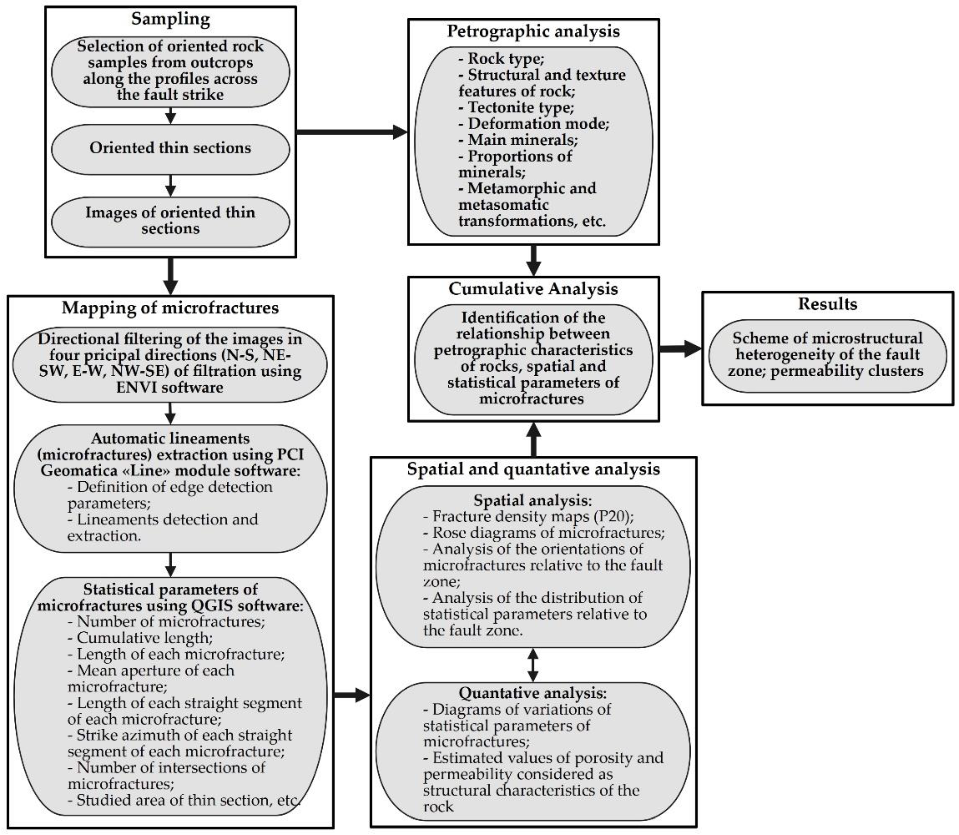
2. Materials and Methods
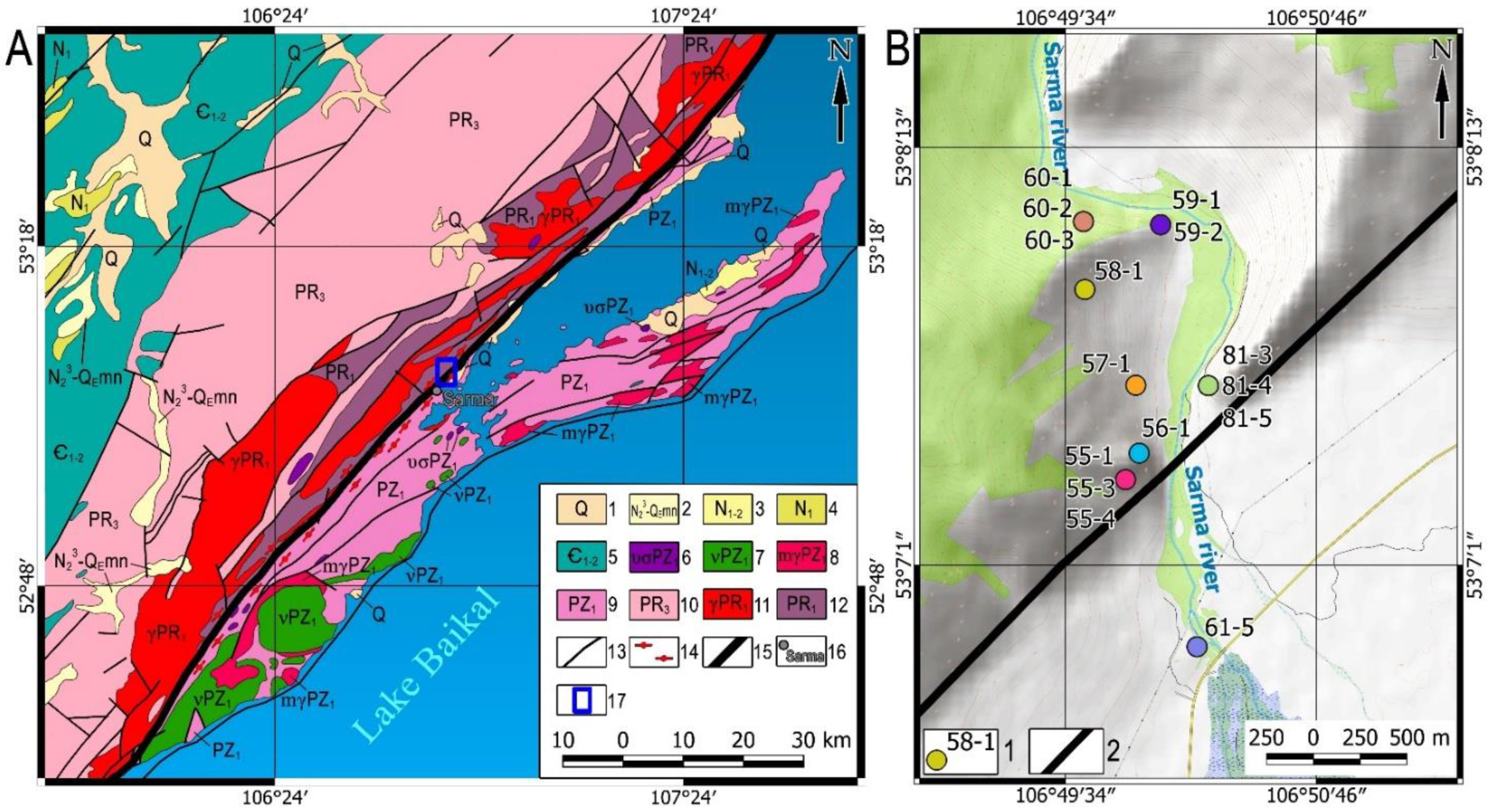
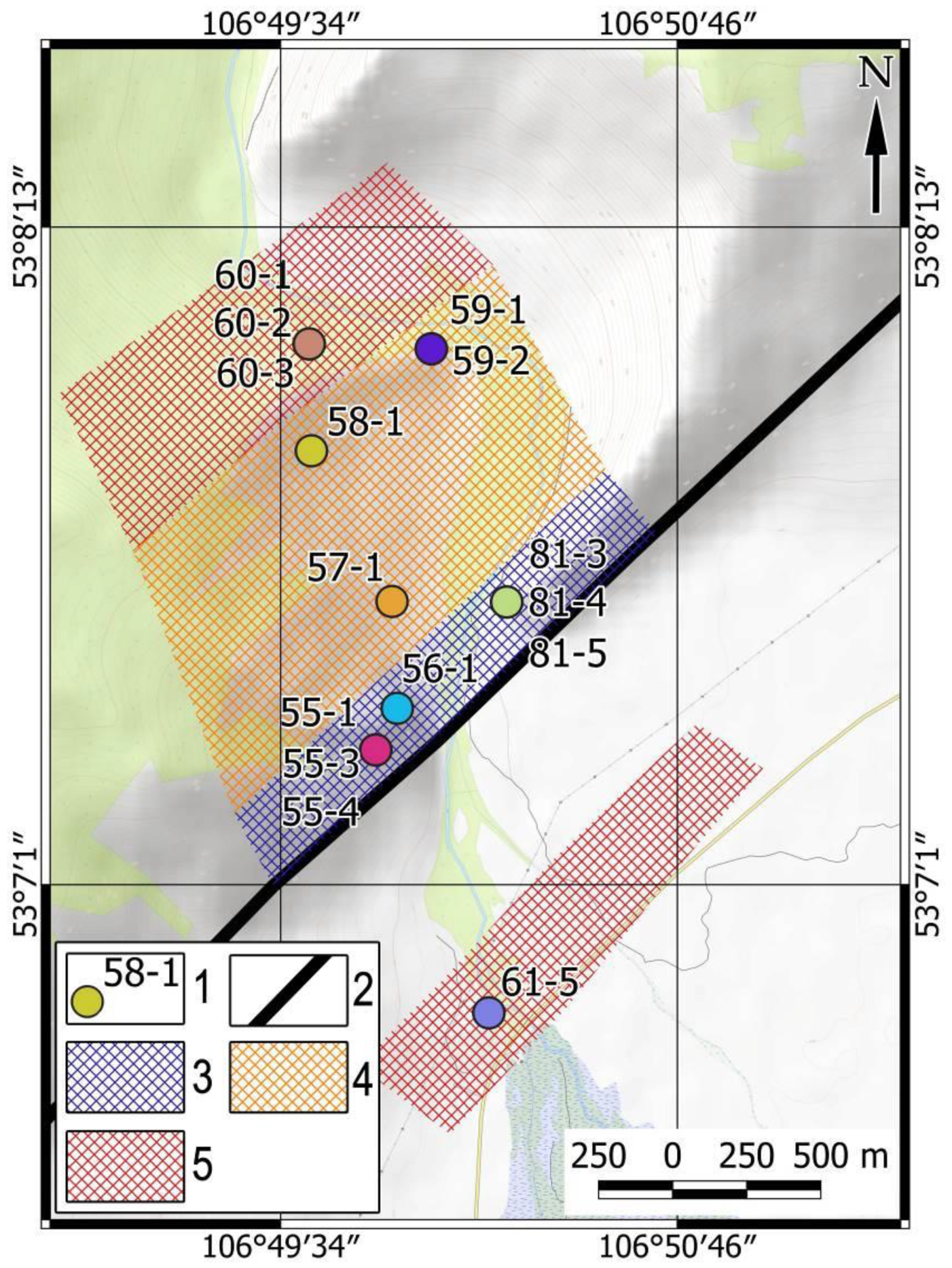
2.1. Area of Study
2.2. Collection of Rock Samples and Petrographic Analysis
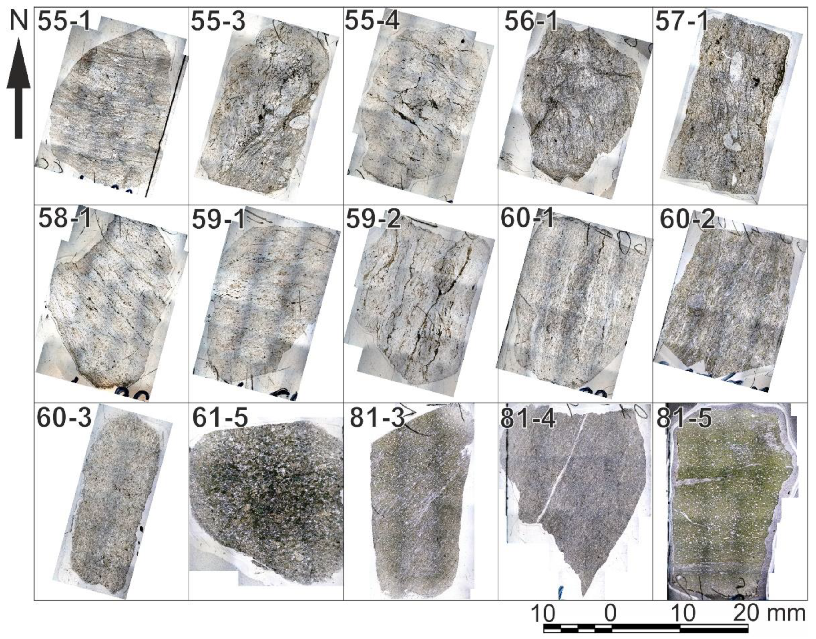
2.3. Fotos of Thin Sections
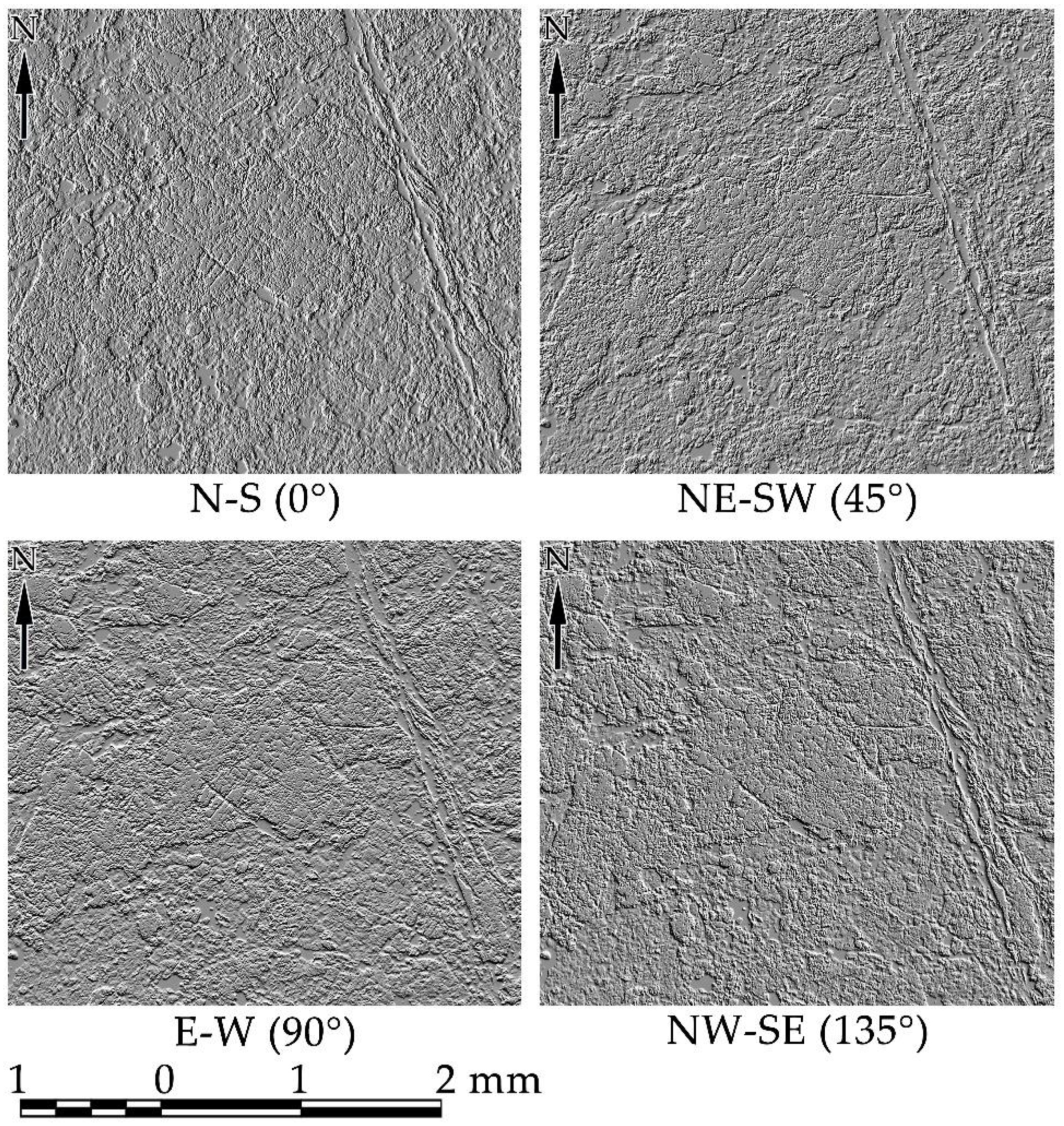
2.4. Special Technique of Microstructural Analysis (STMA)
- Implementation of binding the rasters (images) of individual parts of a thin section, as well as their filling and docking in a single coordinate system;
- Determination of relative coordinates X and Y of any point in a thin section;
- Marking all microstructures within the thin section;
- Automatic determination and measurement of geometrical parameters of microstructures (strike azimuth, length and aperture);
- Identification of various ensembles and microstructure generations depending on the values of azimuth and their separate marking;
- Possibility of marking objects over type (microcracks filled with secondary fluid inclusions (FIPs), open or partially mineralized microcracks and microcracks filled with ore material);
- Calculation of porosity and permeability in paleo and modern conditions at various stages of deformation of geological bodies;
- Determination of quantitative and percent ratios of different types of microstructures and presentation of the results in the form of diagrams (graphs, rose-diagrams and histograms).
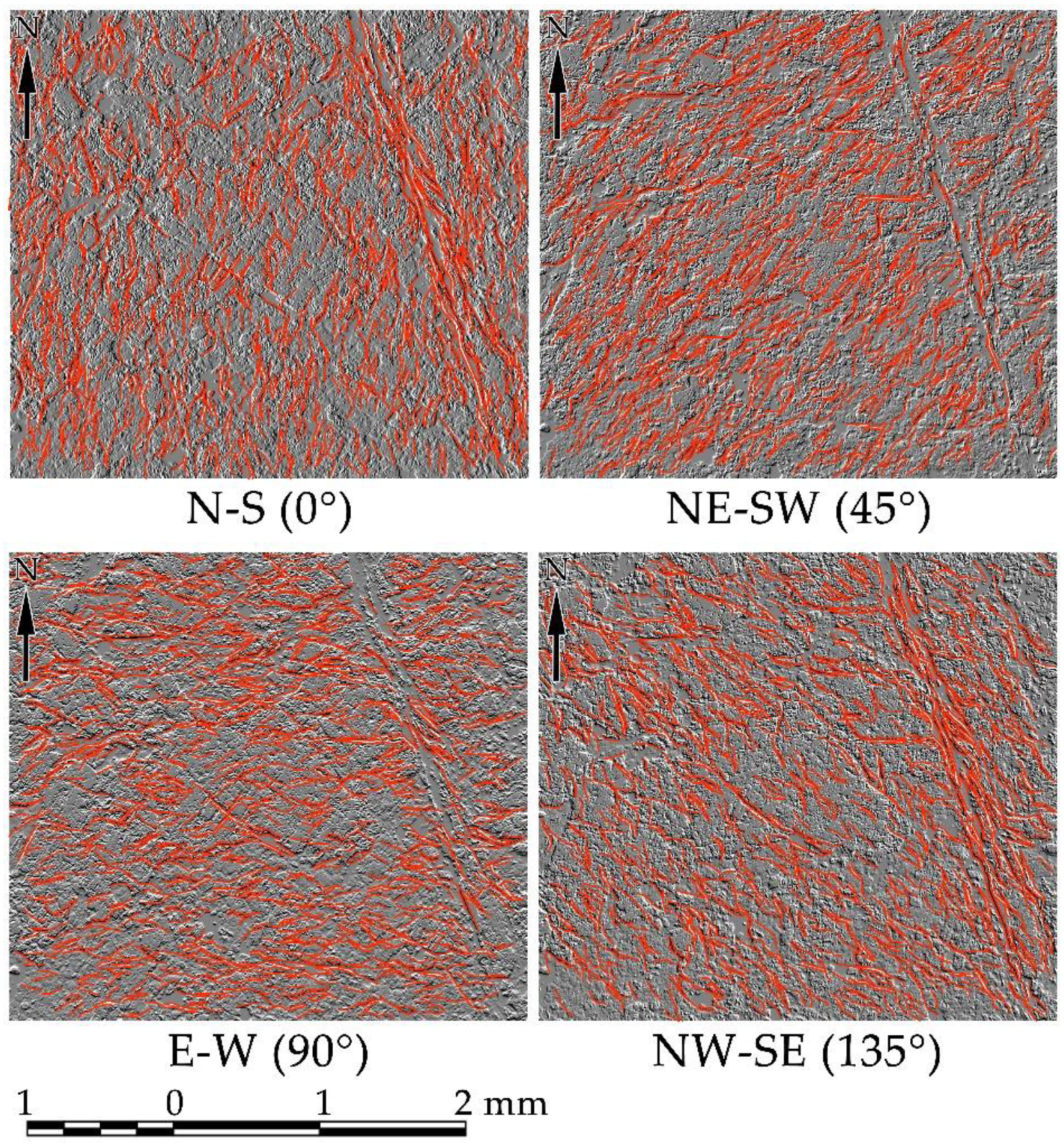
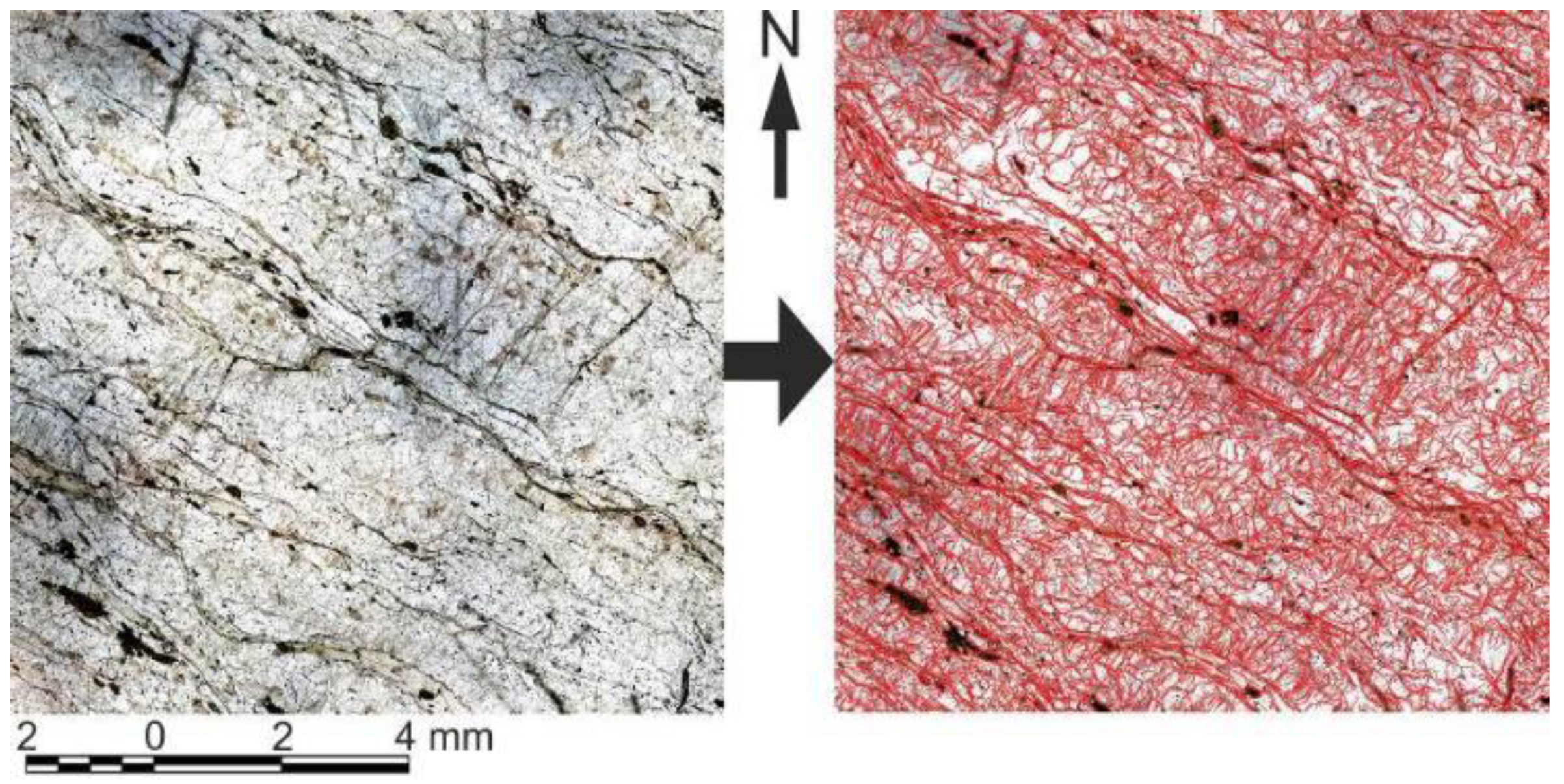
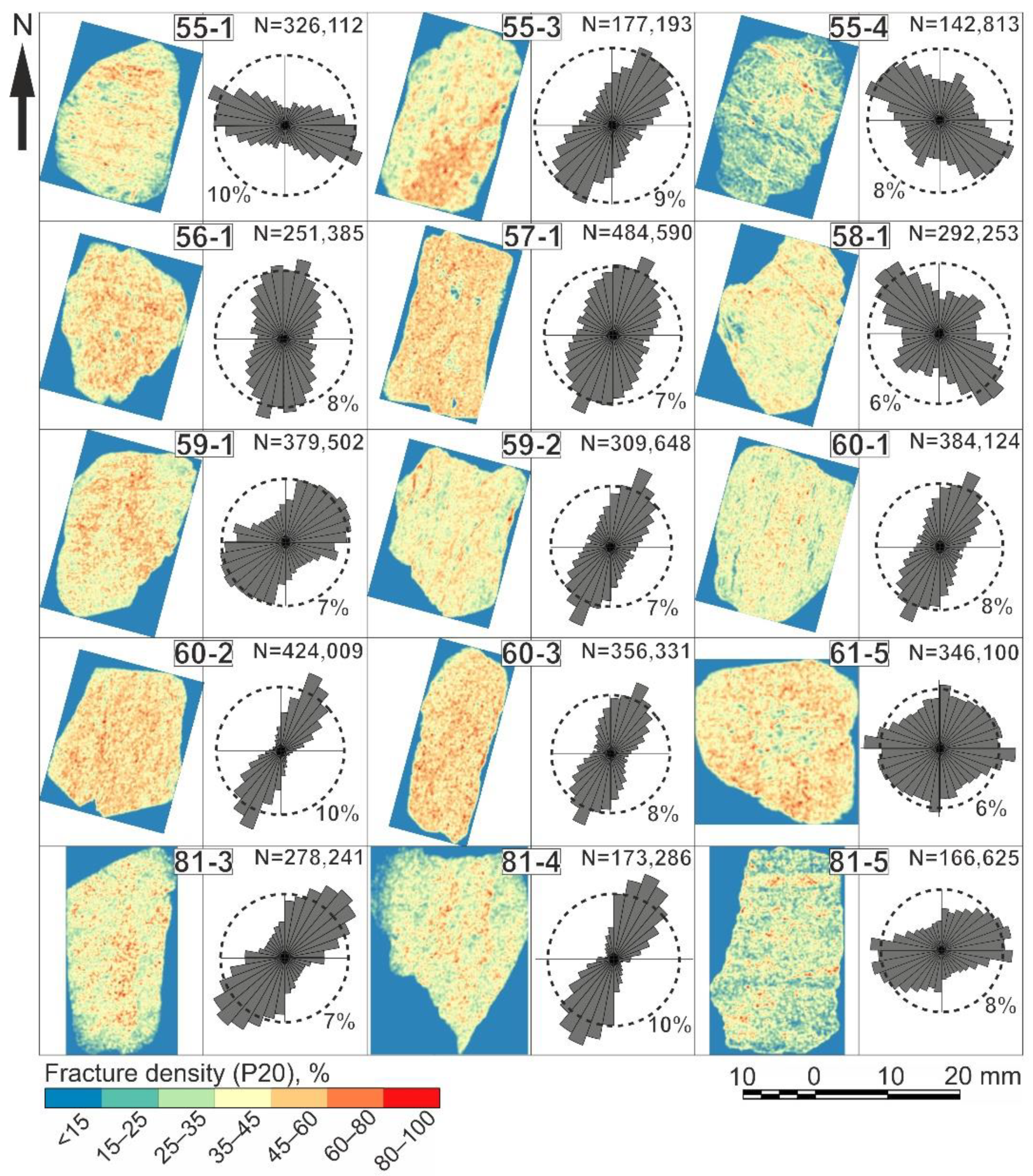
2.4.1. Automatic Mapping of Microfractures
2.4.2. Microfracture Characteristics
- Number of objects (microfractures);
- X and Y coordinates of the ends;
- Cumulative length;
- Length of each microfracture;
- Mean aperture of each microfracture;
- Length of each straight segment of each microfracture;
- Strike azimuth of each straight segment of each microfracture;
- Number of intersections of microfractures;
- Studied area of thin section, etc.
2.4.3. Determination of Porosity and Permeability
3. Results
4. Discussion
5. Conclusions
Author Contributions
Funding
Institutional Review Board Statement
Informed Consent Statement
Data Availability Statement
Acknowledgments
Conflicts of Interest
References
- Stephens, T.L.; Walker, R.J.; Healy, D.; Bubeck, A.; England, R.W. Mechanical models to estimate the paleostress state from igneous intrusions. Solid Earth 2018, 9, 847–858. [Google Scholar] [CrossRef] [Green Version]
- Yamaji, A.; Sato, K. Clustering of fracture orientations using a mixed Bing ham distribution and its application to paleostress analysis from dike or vein orientations. J. Struct. Geol. 2011, 33, 1148–1157. [Google Scholar] [CrossRef] [Green Version]
- De Guidi, G.; Caputo, R.; Scudero, S. Regional and local stress field orientation inferred from quantitative analyses of extension joints: Case study from southern Italy. Tectonics 2013, 32, 239–251. [Google Scholar] [CrossRef] [Green Version]
- Saintot, A.; Angelier, J. Tectonic paleostress fields and structural evolution of the NW-Caucasus fold-and-thrust belt from Late Cretaceous to Quaternary. Tectonophysics 2002, 357, 1–31. [Google Scholar] [CrossRef] [Green Version]
- Sim, L.A. Some methodological aspects of tectonic stress reconstruction based on geological indicators. Comptes Rendus Geosci. 2012, 344, 174–180. [Google Scholar] [CrossRef] [Green Version]
- Bott, M.H.P. The mechanics of obique slip faulting. Geol. Mag. 1959, 96, 109–117. [Google Scholar] [CrossRef]
- Gushchenko, O.I. The method of kinematic analysis of destruction structures in reconstruction of tectonic stress fields. In Fields of Stress and Strain in the Lithosphere; Grigoriev, A.S., Osokina, D.N., Eds.; Nauka: Moscow, Russia, 1979; pp. 7–25. (In Russian) [Google Scholar]
- Rebetskii, Y.L.; Marinin, A.V. Stressed state of the Earth’s crust in the western region of the Sunda subduction zone before the Sumatra-Andaman earthquake on December 26, 2004. Dokl. Earth Sci. 2006, 407, 321–325. [Google Scholar] [CrossRef]
- Gzovsky, M.V. Fundamentals of Tectonophysics; Nauka: Moscow, Russia, 1975; p. 536. (In Russian) [Google Scholar]
- Nikolaev, P.N. Methodology of Tectonodynamic Analysis; Nedra: Moscow, Russia, 1992; p. 295. (In Russian) [Google Scholar]
- Angelier, J. Fault slip analysis and paleostress reconstruction. In Continental Deformation; Hancock, P.L., Ed.; Pergamon Press: Oxford, UK, 1994; pp. 53–100. [Google Scholar]
- Lacombe, O. Do fault slip data inversions actually yield “paleostresses” that can be compared with contemporary stresses? A critical discussion. Comptes Rendus Geosci. 2012, 344, 159–173. [Google Scholar] [CrossRef]
- Heap, M.J.; Kushnir, A.R.L.; Gilg, H.A. Microstructural and petrophysical properties of the Permo-Triassic sandstones (Buntsandstein) from the Soultz-sous-Forêts geothermal site (France). Geotherm. Energy 2017, 5, 26. [Google Scholar] [CrossRef] [Green Version]
- Yang, G.; Leung, A.K.; Xu, N.; Zhang, K.; Gao, K. Three-dimensional physical and numerical modelling of fracturing and deformation behaviour of mining-induced rock slopes. Appl. Sci. 2019, 9, 1360. [Google Scholar] [CrossRef] [Green Version]
- Unver, B.; Yasitli, N. Modelling of strata movement with a special reference to caving mechanism in thick seam coal mining. Int. J. Coal Geol. 2016, 66, 227–252. [Google Scholar] [CrossRef]
- Petrov, V.A.; Poluektov, V.V.; Ustinov, S.A.; Minaev, V.A.; Lespinasse, M. Rescaling of fluid-conducting fault structures. Dokl. Earth Sci. 2017, 472, 130–133. [Google Scholar] [CrossRef]
- Petrov, V.A.; Poluektov, V.V.; Ustinov, S.A.; Minaev, V.A.; Lespinasse, M. Scale effect in a fluid-conducting fault network. Geol. Ore Depos. 2019, 61, 293–305. [Google Scholar] [CrossRef]
- Ben-Zion, Y.; Sammis, C.G. Characterization of fault zones. Pure Appl. Geophys. 2003, 160, 677–715. [Google Scholar] [CrossRef] [Green Version]
- Faulkner, D.R.; Lewis, A.C.; Rutter, E.H. On the internal structure and mechanics of large strike-slip fault zones: Field observations of the Carboneras fault in southeastem Spain. Tectonophysics 2003, 367, 235–251. [Google Scholar] [CrossRef]
- Wibberley, C.A.J.; Shimamoto, T. Internal structure and permeability of major strike-slip fault zones: The Median Tectonic Line in Mie Prefecture, southwest Japan. J. Struct. Geol. 2003, 25, 59–78. [Google Scholar] [CrossRef]
- Mitchell, T.M.; Faulkner, D.R. The nature and origin of off-fault damage surrounding strike-slip fault zones with a wide range of displacements: A field study from the Atacama fault system, northern Chile. J. Struct. Geol. 2009, 31, 802–816. [Google Scholar] [CrossRef]
- Lespinasse, M.; Pecher, A. Microfracturing and regional stress field: A study of the preferred orientation of fluid-inclusion planes in a granite from the Massif Central, France. J. Struct. Geol. 1986, 8, 169–180. [Google Scholar] [CrossRef]
- Boullier, A.-M. Fluid inclusions: Tectonic indicators. J. Struct. Geol. 1999, 21, 1229–1235. [Google Scholar] [CrossRef]
- Wilson, J.E.; Chester, J.S.; Chester, F.M. Microfracture analysis of fault growth and wear processes, Punchbowl Fault, San Andreas system, California. J. Struct. Geol. 2003, 25, 1855–1873. [Google Scholar] [CrossRef]
- Wise, D.U. Microjointing in basement, middle Rocky Mountains of Montana and Wyoming. Geol. Soc. Am. Bull. 1964, 75, 287–306. [Google Scholar] [CrossRef]
- Hoxha, D.; Homand, F. Microstructural approach in damage modeling. Mech. Mater. 2000, 32, 377–387. [Google Scholar] [CrossRef]
- Lespinasse, M.; Désindes, L.; Fratczak, P.; Petrov, V. Microfissural mapping of natural cracks in rocks: Implications for fluid transfers quantification in the crust. Chem. Geol. 2005, 223, 170–178. [Google Scholar] [CrossRef]
- Duarte, M.T.; Liu, H.Y.; Kou, S.Q.; Lindqvist, P.A.; Miskovsky, K. Microstructural modeling approach applied to rock material. J. Mater. Eng. Perform. 2005, 14, 104–111. [Google Scholar] [CrossRef]
- Lukin, L.I.; Chernyshev, V.F.; Kushnarev, I.P. Microstructural Analysis; Nauka: Moscow, Russia, 1965; p. 124. (In Russian) [Google Scholar]
- Costin, L.S. A microcrack model for the deformation and failure of brittle rock. J. Geophys. Res. 1983, 88, 9485–9492. [Google Scholar] [CrossRef]
- Kranz, R.L. Microcracks in rocks: A review. Tectonophysics 1983, 100, 449–480. [Google Scholar] [CrossRef]
- Lawn, B. Fracture of brittle solids. In Cambridge Solid State Science Series, 2nd ed.; Cambridge University Press: Cambridge, UK, 1993; p. 378. [Google Scholar]
- Brandes, C.; Tanner, D.C. Chapter 2—Fault mechanics and earthquakes. In Understanding Faults; Tanner, D., Brandes, C., Eds.; Elsevier: Amsterdam, The Netherlands, 2020; pp. 11–80. [Google Scholar] [CrossRef]
- Jaeger, J.C.; Cook, N.G.W. Fundamentals of Rock Mechanics, 3rd ed.; Chapman and Hall: London, UK, 1979; p. 593. [Google Scholar]
- Buck, W.R. The Dynamics of Continental Breakup and Extensio. In Treatise on Geophysics, 2nd ed.; Schubert, G., Ed.; Elsevier: Amsterdam, The Netherlands, 2015; pp. 325–379. [Google Scholar] [CrossRef]
- Tamanyu, S.; Fujimoto, K. On the models for the deep-seated geothermal system in the Kakkonda field. Rept. Geol. Surv. Jpn. 2000, 284, 133–164. [Google Scholar]
- Fournier, R.O. Hydrothermal processes related to movement of fluid from plastic into brittle rock in the magmatic-epithermal environment. Econ. Geol. 1999, 94, 1193–1211. [Google Scholar] [CrossRef]
- Harvey, P.K.; Brewer, T.S.; Pezard, P.A.; Petrov, V.A. Petrophysical Propoerties of Cristalline Rocks; The Geological Society: London, UK, 2005; p. 345. [Google Scholar]
- Nelson, R.A. Geological Analysis of Naturally Fractured Reservoirs, 2nd ed.; Gulf Professional Publishing: Boston, MA, USA, 2001. [Google Scholar]
- Snow, D.T. Anisotropie permeability of fractured media. Water Resour. Res. 1969, 5, 1273–1289. [Google Scholar] [CrossRef]
- Moench, A.F. Double-porosity models for a fissured groundwater reservoir with fracture skin. Water Resour. Res. 1984, 20, 831–846. [Google Scholar] [CrossRef]
- Ababou, R. Approaches to Large Scale Unsaturated Flow in Heterogeneous Stratified and Fractured Geologic Media; US Nuclear Regulatory Commission: Washington, DC, USA, 1991. [Google Scholar]
- Long, J.C.S.; Gilmour, P.; Whiterspoon, P.A. A model for steady fluid flow in random three-dimensional networks of diskshaped fractures. Water Resour. Res. 1985, 21, 105–115. [Google Scholar] [CrossRef] [Green Version]
- Gueguen, Y.; Dienes, J. Transport properties of rocks from statistics and percolation. Math. Geol. 1989, 21, 1–13. [Google Scholar] [CrossRef]
- Canals, M.; Ayt Ougougdal, M. Percolation on anisotropic media, the Bethe lattice revisited. Application to fracture networks. Nonlinear Processes Geophys. 1997, 4, 11–18. [Google Scholar] [CrossRef] [Green Version]
- Stauffer, D. Introduction to Percolation Theory; Taylor and Francis: London, UK, 1985; p. 124. [Google Scholar]
- Homand, F.; Hoxha, D.; Belem, T.; Pons, M.N.; Hoteit, N. Geometric analysis of damaged microcracking in granites. Mech. Mater. 2000, 32, 361–376. [Google Scholar] [CrossRef]
- Lespinasse, M.; Sausse, J. Quantification of fluid flow: Hydromechanical behaviour of different natural rough fractures. J. Geochem. Explor. 2000, 69–70, 483–486. [Google Scholar] [CrossRef]
- Sausse, J.; Jacquot, E.; Fritz, B.; Leroy, J.; Lespinasse, M. Evolution of crack permeability during fluid-rock interaction. Example of the Brézouard granite (Vosges, France). Tectonophysics 2001, 336, 199–214. [Google Scholar] [CrossRef]
- Sausse, J. Hydromechanical properties and alteration of natural fracture surfaces in the Soultz granite (Bas-Rhin, France). Tectonophysics 2002, 348, 169–185. [Google Scholar] [CrossRef]
- Zhang, L.; Einstein, H.H. Estimating the intensity of rock discontinuities. Int. J. Rock Mech. Min. Sci. 2000, 37, 819–837. [Google Scholar] [CrossRef]
- Zhang, L.; Einstein, H.H. Estimating the mean trace length of rock discontinuities. Rock Mech. Rock Eng. 1998, 31, 217–235. [Google Scholar] [CrossRef]
- Riley, M.S. Fracture trace length and number distributions from fracture mapping. J. Geophys. Res. 2005, 110, B08414. [Google Scholar] [CrossRef]
- Zeeb, C.; Gomez-Rivas, E.; Bons, P.D.; Blum, P. Evaluation of sampling methods for fracture network characterization using outcrops. AAPG Bull. 2013, 97, 1545–1566. [Google Scholar] [CrossRef]
- Hirono, T.; Takahashi, M.; Nakashima, S. In situ visualization of fluid flow image within deformed rock by X-ray CT. Eng. Geol. 2003, 70, 37–46. [Google Scholar] [CrossRef]
- Menendez, B.; David, D.; Martı’nez Nistal, A. Confocal scanning laser microscopy applied to the study of pore and crack networks in rocks. Comput. Geosci. 2001, 27, 1101–1109. [Google Scholar] [CrossRef]
- Geraud, Y.; Caron, J.M.; Faure, P. Porosity network of a ductile shear zone. J. Struct. Geol. 1995, 17, 1757–1769. [Google Scholar] [CrossRef]
- Passchier, C.W.; Trouw, R.A.J. Microtectonics, 2nd ed.; Springer: Berlin, Germany, 2005; p. 366. [Google Scholar]
- Ustinov, S.; Petrov, V.; Poluektov, V.; Minaev, V. Calculation of filtration properties of the Antey uranium deposit rock massif at the deformation phases: Microstructural approach. In Trigger Effects in Geosystems; Kocharyan, G., Lyakhov, A., Eds.; Springer Nature: Cham, Switzerland, 2019; pp. 179–186. [Google Scholar]
- Xu, J.; Zhao, X.; Liu, B. Digital image analysis of fluid inclusions. Int. J. Rock Mech. Min. Sci. 2007, 44, 942–947. [Google Scholar] [CrossRef]
- Healy, D.; Rizzo, R.E.; Cornwell, D.G.; Farrell, N.J.C.; Watkins, H.; Timms, N.E.; Gomez-Rivas, E.; Smith, M. FracPaQ: A MATLAB™ toolbox for the quantification of fracture patterns. J. Struct. Geol. 2017, 95, 1–16. [Google Scholar] [CrossRef] [Green Version]
- Zeeb, C.; Gomez-Rivas, E.; Bons, P.D.; Virgo, S.; Blum, P. Fracture network evaluation program (FraNEP): A software for analyzing 2D fracture trace-line maps. Comput. Geosci. 2013, 60, 11–22. [Google Scholar] [CrossRef]
- Xu, C.; Dowd, P. A new computer code for discrete fracture network modelling. Comput. Geosci. 2010, 36, 292–301. [Google Scholar] [CrossRef]
- Saha, K.; Frøyen, Y.K. Learning GIS Using Open Source Software, 1st ed.; Taylor and Francis Group: London, UK, 2021; p. 240. [Google Scholar] [CrossRef]
- Longley, P.A.; Goodchild, M.F.; Maguire, D.J.; Rhind, D.W. Geographic Information Systems and Science, 2nd ed.; John Wiley and Sons: Chichester, UK, 2005. [Google Scholar]
- Chang, K. Introduction to Geographic Information System, 4th ed.; McGraw-Hill Education: New York, NY, USA, 2016; p. 249. [Google Scholar]
- Best, M.G. Igneous and Metamorphic Petrology, 2nd ed.; Blackwell Publishing Company: Oxford, UK, 2003; p. 752. [Google Scholar]
- Letnikov, F.A.; Balyshev, S.O. Petrophysics and Geoenergetics of Tectonites; Nauka: Novosibirsk, Russia, 1991; p. 148. (In Russian) [Google Scholar]
- Sherman, S.I. Physics of Crustal Faulting; Nauka: Novosibirsk, Russia, 1977; p. 102. (In Russian) [Google Scholar]
- Mats, V.D. The Cenozoic History and Structure of the Baikal Rift Basin; GEO: Novosibirsk, Russia, 2001; p. 252. (In Russian) [Google Scholar]
- Lunina, O.V.; Gladkov, A.S.; Cheremnykh, A.V. Fracturing in the Primorsky fault zone (Baikal Rift system). Russ. Geol. Geophys. 2002, 43, 446–455. [Google Scholar]
- Mats, V.D.; Lobatskaya, R.M.; Khlystov, O.M. Evolution of faults in continental rifts: Morphotectonic evidence from the south-western termination of the North Baikal basin. Earth Sci. Front. 2007, 14, 207–219. [Google Scholar] [CrossRef]
- Cheremnykh, A.V. Stress fields in the Primorsky normal fault zone (Baikal rift). Lithosfera 2011, 1, 135–142. [Google Scholar]
- Cheremnykh, A.V.; Cheremnykh, A.S.; Bobrov, A.A. Faults in the Baikal region: Morphostructural and structure-genetic features (case study of the Buguldeika fault junction). Russ. Geol. Geophys. 2018, 59, 1100–1108. [Google Scholar] [CrossRef]
- Cheremnykh, A.V.; Burzunova, Y.P.; Dekabryov, I.K. Hierarchic features of stress field in the Baikal region: Case study of the Buguldeika Fault Junction. J. Geodyn. 2020, 141–142, 101797. [Google Scholar] [CrossRef]
- Seminskii, K.Z.; Kozhevnikov, N.O.; Cheremnykh, A.V.; Pospeeva, E.V.; Bobrov, A.A.; Olenchenko, V.V.; Tugarina, M.A.; Potapov, V.V.; Burzunova, Y.P. Interblock zones of the northwestern Baikal rift: Results of geological and geophysical studies along the Bayandai Village—cape Krestovskii profile. Russ. Geol. Geophys. 2012, 53, 194–208. [Google Scholar] [CrossRef]
- Lamakin, V.V. Neotectonics of the Baikal Basin; Nauka: Moscow, Russia, 1968; p. 247. (In Russian) [Google Scholar]
- Aleksandrov, V.K. Thrusts in the Baikal Region; Nauka: Novosibirsk, Russia, 1990; p. 102. (In Russian) [Google Scholar]
- Delvaux, D.; Moeys, R.; Stapel, G.; Melnikov, A.; Ermikov, V. Paleostress reconstructions and geodynamics of the Baikal region, Central Asia. Part I: Palaeozoic and Mesozoic pre-rift evolution. Tectonophysics 1995, 252, 61–101. [Google Scholar] [CrossRef]
- Delvaux, D.; Moyes, R.; Stapel, G.; Petit, C.; Levi, K.; Miroshnitchenko, A.; Ruzhich, V.; San’kov, V. Paleostress reconstruction and geodynamics of the Baikal region, Central Asia. Part II: Cenozoic rifting. Tectonophysics 1997, 282, 1–38. [Google Scholar] [CrossRef]
- Gladkochub, D.P.; Donskaya, T.V.; Wingate, M.T.D.; Poller, U.; Kr¨oner, A.; Fedorovsky, V.S.; Mazukabzov, A.M.; Todt, W.; Pisarevsky, S.A. Petrology, geochronology, and tectonic implications of ca. 500 Ma metamorphic and igneous rocks along the northern margin of the Central-Asian Orogen (Olkhon terrane, Lake Baikal, Siberia). J. Geol. Soc. Lond. 2008, 165, 235–246. [Google Scholar] [CrossRef]
- Gladkochub, D.P.; Donskaya, T.V.; Mazukabzov, A.M.; Sklyarov, E.V.; Fedorovskii, V.S.; Lavrenchuk, A.V.; Lepekhina, E.N. Fragment of the Early Paleozoic (~500 Ma) island arc in the structure of the Olkhon terrane, Central Asian fold belt. Dokl. Earth Sci. 2014, 457, 905–909. [Google Scholar] [CrossRef]
- Donskaya, T.V.; Gladkochub, D.P.; Mazukabzov, A.M.; Fedorovsky, V.S.; Cho, M.; Cheong, W.; Kim, J. Synmetamorphic granitoids (~490 Ma) as accretion indicators in the evolution of the Olkhon terrane (Western Cisbaikalia). Russ. Geol. Geophys. 2013, 54, 1205–1218. [Google Scholar] [CrossRef]
- Donskaya, T.V.; Gladkochub, D.P.; Fedorovsky, V.S.; Sklyarov, E.V.; Cho, M.; Sergeev, S.A.; Demonterova, E.I.; Mazukabzov, A.M.; Lepekhina, E.N.; Cheong, W.; et al. Pre-collisional (& 0.5 Ga) complexes of the Olkhon terrane (southern Siberia) as an echo of events in the Central Asian Orogenic Belt. Gondwana Res. 2017, 42, 243–263. [Google Scholar] [CrossRef]
- Mats, V.D.; Perepelova, T.I. A new perspective on evolution of the Baikal Rift. Geosci. Front. 2011, 2, 349–365. [Google Scholar] [CrossRef] [Green Version]
- Ruzhich, V.V.; Kocharyan, G.G.; Savelieva, V.B.; Travin, A.V. On the structure and formation of earthquake sources in the faults located in the subsurface and deep levels of the crust. Part II. Deep level. Geodyn. Tectonophys. 2018, 9, 1039–1061. [Google Scholar] [CrossRef]
- Lauf, G.B. The Transverse Mercator projection. S. Afr. Geogr. J. 2012, 57, 118–125. [Google Scholar] [CrossRef]
- Suzen, M.L.; Toprak, V. Filtering of Satellite Images in Geological Lineament Analyses: An Application to a Fault Zone in Central Turkey. Int. J. Remote Sens. 1998, 19, 1101–1114. [Google Scholar] [CrossRef]
- Gloaguen, R.; Marpu, P.R.; Niemeyer, I. Automatic extraction of faults and fractal analysis from remote sensing data. Nonlinear Process. Geophys. 2007, 14, 131–138. [Google Scholar] [CrossRef]
- Sedrette, S.; Rebai, N. Assessment Approach for the Automatic Lineaments Extraction Results Using Multisource Data and GIS Environment: Case Study in Nefza Region in North-West of Tunisia. In Mapping and Spatial Analysis of Socio-Economic and Environmental Indicators for Sustainable Development. Advances in Science, Technology & Innovation (IEREK Interdisciplinary Series for Sustainable Development; Rebai, N., Mastere, M., Eds.; Springer: Berlin, Germany, 2019; pp. 63–69. [Google Scholar] [CrossRef]
- Enoh, M.A.; Okeke, F.I.; Okeke, U.C. Automatic lineaments mapping and extraction in relationship to natural hydrocarbon seepage in Ugwueme, South-Eastern Nigeria. Geod. Cartogr. 2021, 47, 34–44. [Google Scholar] [CrossRef]
- Paplinski, A. Directional filtering in edge detection. IEEE Trans. Image Processing 1998, 7, 611–615. [Google Scholar] [CrossRef] [Green Version]
- Salui, C.L. Methodological validation for automated lineament extraction by LINE method in PCI Geomatica and MATLAB based Hough transformation. J. Geol. Soc. India 2018, 92, 321–328. [Google Scholar] [CrossRef]
- QGIS User Guide—QGIS Documentation. Available online: https://docs.qgis.org/3.16/en/docs/user_manual/index.html (accessed on 21 January 2022).
- Underwood, E.E. Quantitative Microscopy; DeHoff, R.T., Rhines, F.N., Eds.; McGraw-Hill Book Co.: New York, NY, USA, 1968; p. 149. [Google Scholar]
- Brace, W.F. Permeability of crystalline rocks: New in situ measurements. J. Geophys. Res. 1984, 89, 4327–4330. [Google Scholar] [CrossRef]
- Gueguen, Y.; Shubnel, Y. Elastic wave velocities and permeability of cracked rocks. Tectonophysics 2003, 370, 163–176. [Google Scholar] [CrossRef]
- Shmonov, V.M.; Vitovtova, V.M.; Zharikov, A.V. Fluid permeability of Rocks of the Earth’s Crust; Scientific World: Moscow, Russia, 2002; p. 216. (In Russian) [Google Scholar]
- Ortega, O.J.; Marrett, R.A.; Laubach, S.E. A scale-independent approach to fracture intensity and average spacing measurement. AAPG Bull. 2006, 90, 193–208. [Google Scholar] [CrossRef]
- Bisdom, K.; Gauthier, B.D.M.; Bertotti, G.; Hardebol, N.J. Calibrating discrete fracture-network models with a carbonate three-dimensional outcrop fracture network: Implications for naturally fractured reservoir modeling. AAPG Bull. 2014, 98, 1351–1376. [Google Scholar] [CrossRef]
- Rebetsky, Y.L.; Sim, L.A.; Marinin, A.V. From Slickensides to Tectonic Stresses. Methods and Algorithms; GEOS Publishing House: Moscow, Russia, 2017; p. 234. (In Russian) [Google Scholar]
- Petrov, V.A.; Sim, L.A.; Nasimov, R.M.; Shchukin, S.I. Fault tectonics, neotectonic stresses, and hidden uranium mineralization in the area adjacent to the Strel’tsovka Caldera. Geol. Ore Depos. 2010, 52, 279–288. [Google Scholar] [CrossRef]


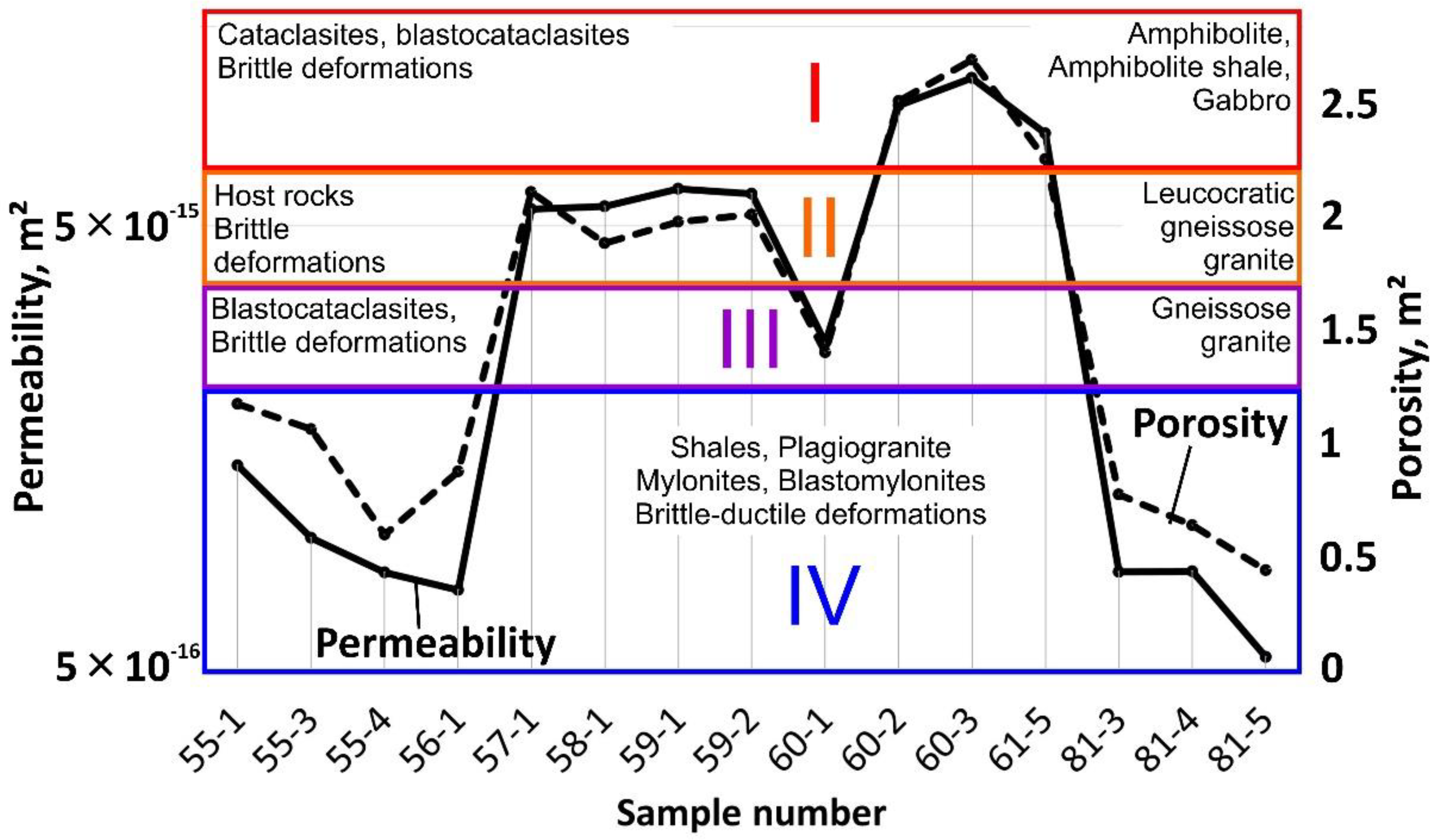
| Sample Number | Petrographic Type | Tectonite Type | Deformation Mode | Main Minerals * and Proportions (%) | Metamorphic and Metasomatic Transformations |
|---|---|---|---|---|---|
| 55-1 | Quartz-Sericite-Chlorite shale | Blastomylonite | Brittle | Q(60), Fsp(20), Src(10), Cl(5) | Complete recrystallization of quartz; sericite is formed by plagioclase; actinolite is chloritized |
| 55-3 | Contact rock: Quartz-Actinolite-Chlorite shale–Plagiogranite | Blastomylonite | Brittle and ductile | Fsp(60), Q(30), Cl(5), Ac(3) | Partial recrystallization of quartz; sericite is formed by plagioclase; actinolite is chloritized |
| 55-4 | Plagiogranite | Mylonite | Brittle | Q(60), Fsp(30), Ac(5), Cl(3), Src(2) | Partial recrystallization of quartz; sericite is formed by plagioclase |
| 56-1 | Plagioamphibo-lite shale | Mylonite | Brittle | Q(50), Fsp(40), Src(5), Cl(3), Ac(2) | Partial recrystallization of quartz; sericite is formed by plagioclase; actinolite is chloritized |
| 57-1 | Chlorite-Sericite-Plagioquartzite shale | Blastocataclasite | Brittle | Q(50), Fsp(30), Src(15), Cl(5), Ac(<1) | Partial recrystallization of quartz; sericite is formed by plagioclase; actinolite is chloritized |
| 58-1 | Leucocratic gneissose granite | Host rock | Brittle | Q(55), Fsp(35), Mu(2), Bt(2) Am(1) | Quartz is slightly granular |
| 59-1 | Leucocratic gneissose granite | Host rock | Brittle | Q(50), Fsp(35), Mu(5), Bt(4) Am(1) | Quartz is slightly granular |
| 59-2 | Leucocratic gneissose granite | Host rock | Brittle | Q(50), Fsp(35), Mu(7), Bt(5) Am(3) | Quartz is slightly granulated; about 10% potassium feldspar saussuritized |
| 60-1 | Gneissose granite | Host rock | Brittle | Q(55), Fsp(30), Bt(10) | Saussurite developed according to potassium feldspar; quartz is slightly granulated |
| 60-2 | Amphibolite | Cataclasite | Ductile | Am(55), Ep(25) Q(15), Fsp(5) | Recrystallization of quartz by schistosity |
| 60-3 | Amphibolite shale | Cataclasite | Ductile | Bt(50), Am(40), Q(5), Fsp(5) | Recrystallization of quartz by schistosity; amphibole is replaced by biotite |
| 61-5 | Gabbro | Blastocataclasite | Brittle | Am(35), Fsp(30), Px(25), Bt(5), Q(5) | Amphibole is substituted with biotite; quartz is recrystallized and switched into the matrix |
| 81-3 | Epidote shale | Blastomylonite | Brittle and ductile | Ep(60), Cl(30), Q(5), | Zone of stress metamorphism; a matrix of ground material of hydromicas formed over amphiboles; quartz is granulated |
| 81-4 | Amphibolite shale | Mylonite | Brittle and ductile | Cl(40), Fsp(20), Am(10), Ep(20), Q(10) | Zone of stress metamorphism; amphibole is replaced by chlorite and stretched into ribbons; Matrix–ground materials of potassium feldspar, chlorite, iron hydroxide |
| 81-5 | Epidote shale | Blastomylonite | Brittle and ductile | Ep(35), Q(15), Cl(40), Ca(10) | Zone of stress metamorphism; a matrix of ground material of hydromicas formed over amphiboles; quartz is granulated |
| Z1 | Z2 | Z3 |
| Z4 | Z5 | Z6 |
| Z7 | Z8 | Z9 |
| N-S (0°) | NE-SW (45°) | E-W (90°) | NW-SE (135°) | ||||||||
|---|---|---|---|---|---|---|---|---|---|---|---|
| −1 | 0 | 1 | −2 | −1 | 0 | −1 | −2 | −1 | 0 | 1 | 2 |
| −2 | 0 | 2 | −1 | 0 | 1 | 0 | 0 | 0 | −1 | 0 | 1 |
| −1 | 0 | 1 | 0 | 1 | 2 | 1 | 2 | 1 | −2 | −1 | 0 |
| Parameter | Description | Range and Unit |
|---|---|---|
| Edge Detection | ||
| RADI | Filter radius. It specifies the radius of the edge detection filter (Filter de Canny). | 0–8192 (pixel) |
| GTHR | Gradient threshold. It specifies the threshold for the minimum gradient level for an edge pixel to obtain a binary image (Filter de Canny). | 0–255 |
| Curve extraction | ||
| LTHR | Length threshold: It specifies the minimum length of curve to be considered as lineament | 0–8192 (pixel) |
| FTHR | Line fitting error threshold: It specifies the maximum error (in pixels) allowed in fitting a polyline to a pixel curve. | 0–8192 (pixel) |
| ATHR | Angular difference threshold: It is the maximum angle between two vectors for them to be linked. | 0–90 (degrees) |
| DTHR | Linking distance threshold: It specifies the minimum distance between the end points of two vectors for them to be linked. | 0–8192 (pixel) |
| Thresholds and Units | Default Value | Verified Value |
|---|---|---|
| RADI (pixels) | 10 | 10 |
| GTHR | 100 | 35 |
| LTHR (pixels) | 30 | 60 |
| FTHR (pixels) | 3 | 5 |
| ATHR (degrees) | 30 | 45 |
| DTHR (pixels) | 20 | 20 |
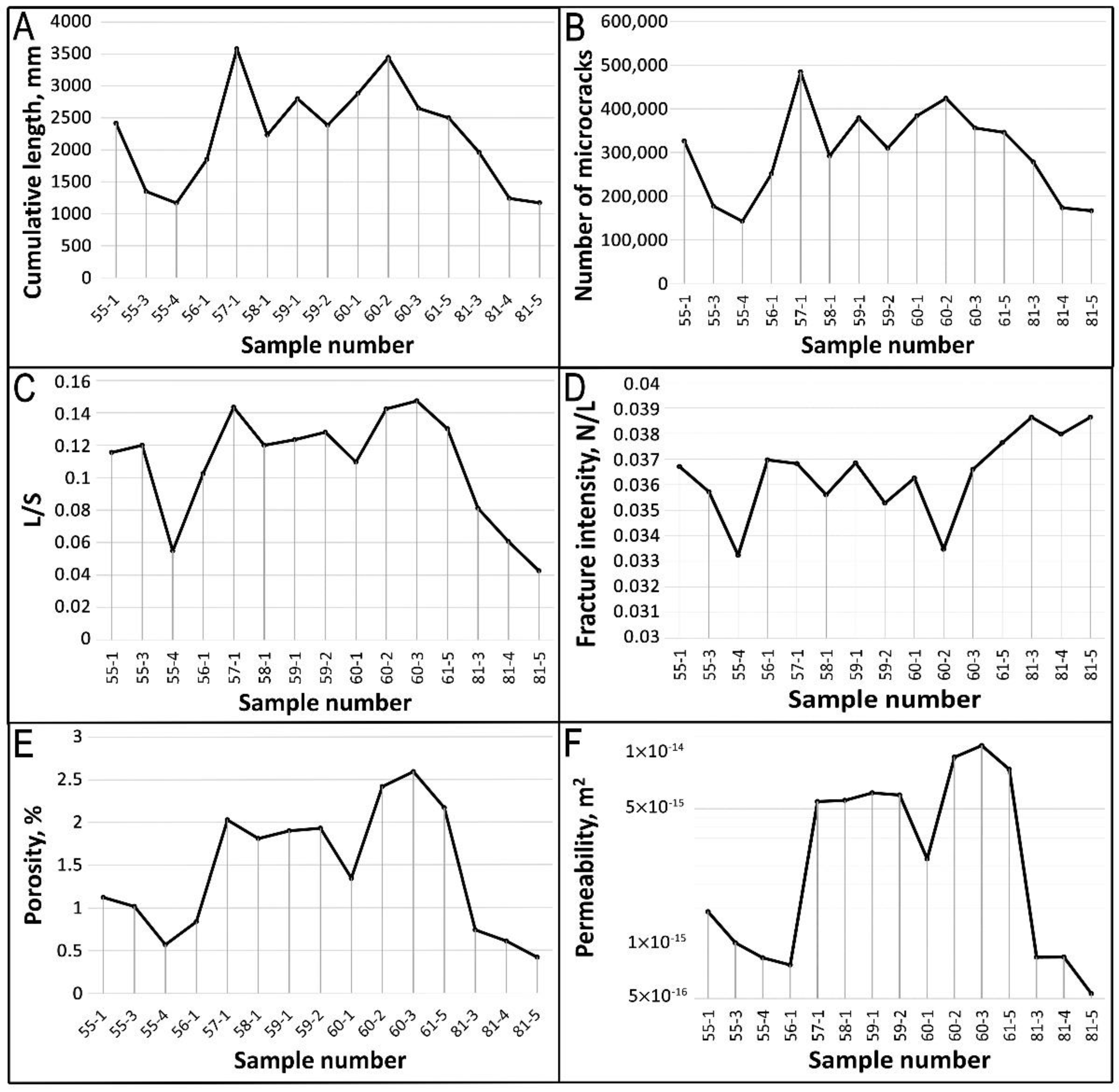
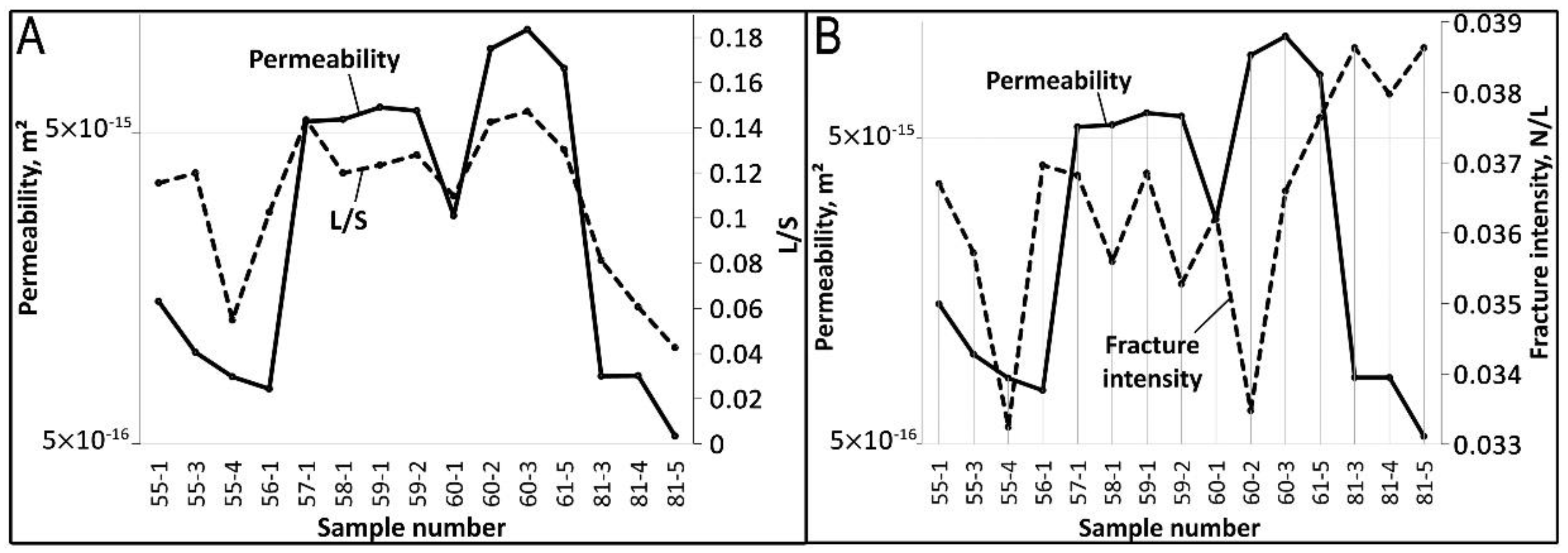
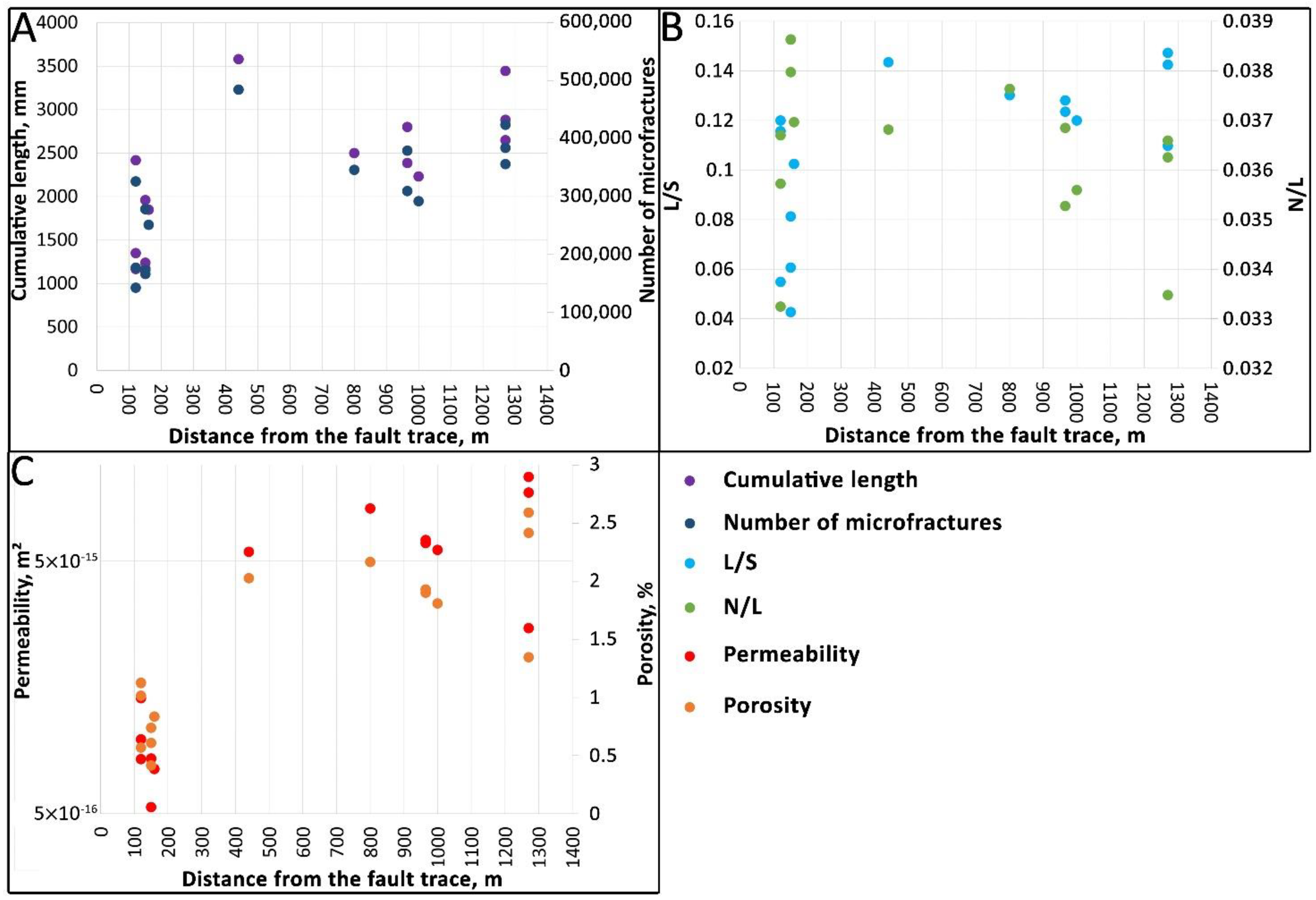
| Sample Number | Cumulative Length, mm (L) | Mean Aperture, Microns (e) | Number of Objects (N) | Studied Area, mm2 (S) | Fracture Intensity F = N/L | L/S | Porosity, % | Permeability, m2 |
|---|---|---|---|---|---|---|---|---|
| 55-1 | 2416.76 | 3.1 | 326,112 | 282.52 | 0.0367 | 0.1156 | 1.13 | 1.44 × 10⁻¹⁵ |
| 55-3 | 1349.20 | 2.7 | 177,193 | 151.99 | 0.0357 | 0.1200 | 1.02 | 9.84 × 10⁻¹⁶ |
| 55-4 | 1168.48 | 3.3 | 142,813 | 287.83 | 0.0332 | 0.0549 | 0.57 | 8.22 × 10⁻¹⁶ |
| 56-1 | 1849.79 | 2.6 | 251,385 | 243.86 | 0.0369 | 0.1025 | 0.84 | 7.52 × 10⁻¹⁶ |
| 57-1 | 3579.96 | 4.5 | 484,590 | 337.23 | 0.0368 | 0.1435 | 2.03 | 5.45 × 10⁻¹⁵ |
| 58-1 | 2233.05 | 4.8 | 292,253 | 251.44 | 0.0356 | 0.1200 | 1.81 | 5.53 × 10⁻¹⁵ |
| 59-1 | 2801.10 | 4.9 | 379,502 | 306.55 | 0.0369 | 0.1235 | 1.90 | 6.05 × 10⁻¹⁵ |
| 59-2 | 2387.49 | 4.8 | 309,648 | 251.95 | 0.0353 | 0.1281 | 1.93 | 5.90 × 10⁻¹⁵ |
| 60-1 | 2881.68 | 3.9 | 384,124 | 354.89 | 0.0363 | 0.1098 | 1.34 | 2.71 × 10⁻¹⁵ |
| 60-2 | 3444.97 | 5.4 | 424,009 | 326.80 | 0.0335 | 0.1425 | 2.42 | 9.35 × 10⁻¹⁵ |
| 60-3 | 2648.34 | 5.6 | 356,331 | 242.95 | 0.0366 | 0.1473 | 2.59 | 1.08 × 10⁻¹⁴ |
| 61-5 | 2501.05 | 5.3 | 346,100 | 259.61 | 0.0376 | 0.1302 | 2.17 | 8.08 × 10⁻¹⁵ |
| 81-3 | 1958.90 | 2.9 | 278,241 | 325.88 | 0.0386 | 0.0812 | 0.74 | 8.26 × 10⁻¹⁶ |
| 81-4 | 1241.22 | 3.2 | 173,286 | 276.85 | 0.0380 | 0.0606 | 0.61 | 8.27 × 10⁻¹⁶ |
| 81-5 | 1173.13 | 3.1 | 166,625 | 371.26 | 0.0386 | 0.0427 | 0.42 | 5.30 × 10⁻¹⁶ |
Publisher’s Note: MDPI stays neutral with regard to jurisdictional claims in published maps and institutional affiliations. |
© 2022 by the authors. Licensee MDPI, Basel, Switzerland. This article is an open access article distributed under the terms and conditions of the Creative Commons Attribution (CC BY) license (https://creativecommons.org/licenses/by/4.0/).
Share and Cite
Ustinov, S.; Ostapchuk, A.; Svecherevskiy, A.; Usachev, A.; Gridin, G.; Grigor’eva, A.; Nafigin, I. Prospects of Geoinformatics in Analyzing Spatial Heterogeneities of Microstructural Properties of a Tectonic Fault. Appl. Sci. 2022, 12, 2864. https://doi.org/10.3390/app12062864
Ustinov S, Ostapchuk A, Svecherevskiy A, Usachev A, Gridin G, Grigor’eva A, Nafigin I. Prospects of Geoinformatics in Analyzing Spatial Heterogeneities of Microstructural Properties of a Tectonic Fault. Applied Sciences. 2022; 12(6):2864. https://doi.org/10.3390/app12062864
Chicago/Turabian StyleUstinov, Stepan, Alexey Ostapchuk, Alexey Svecherevskiy, Alexey Usachev, Grigorii Gridin, Antonina Grigor’eva, and Igor Nafigin. 2022. "Prospects of Geoinformatics in Analyzing Spatial Heterogeneities of Microstructural Properties of a Tectonic Fault" Applied Sciences 12, no. 6: 2864. https://doi.org/10.3390/app12062864