No-Reference Image Quality Assessment Based on Image Multi-Scale Contour Prediction

Abstract

Accurately assessing image quality is a challenging task, especially without a reference image. Currently, most of the no-reference image quality assessment methods still require reference images in the training stage, but reference images are usually not available in real scenes. In this paper, we proposed a model named MSIQA inspired by biological vision and a convolution neural network (CNN), which does not require reference images in the training and testing phases. The model contains two modules, a multi-scale contour prediction network that simulates the contour response of the human optic nerve to images at different distances, and a central attention peripheral inhibition module inspired by the receptive field mechanism of retinal ganglion cells. There are two steps in the training stage. In the first step, the multi-scale contour prediction network learns to predict the contour features of images in different scales, and in the second step, the model combines the central attention peripheral inhibition module to learn to predict the quality score of the image. In the experiments, our method has achieved excellent performance. The Pearson linear correlation coefficient of the MSIQA model test on the LIVE database reached 0.988.

1. Introduction

Image is an important source of information for human perception and machine recognition [1,2,3]. In order for machines to have visual perception, not only does the equipment need to be capable of predictive maintenance [4], but it also needs to capture high-quality images. Image quality plays a decisive role in the sufficiency and accuracy of the acquired information. However, the image is inevitably distorted in the process of acquisition, compression, processing, transmission, and display. How to measure the quality of the image and evaluate whether the image meets a specific requirement becomes a problem. To solve this problem, it is necessary to establish an effective image quality assessment (IQA) system. At present, IQA methods can be divided into subjective evaluation methods and objective evaluation methods. The former relies on the subjective perception of experimenters to evaluate the quality of the object. The latter simulates the perception mechanism of the human visual system based on the quantitative indicators given by the model. According to the classification of images, IQA can be divided into facial image quality [5,6], synthetic image quality, and so on. Below, we introduce the perspective of model improvement.

Objective image quality assessments are quite meaningful. They can provide feedback and optimization for denoising algorithms, provide early evaluation and preprocessing of image data for computer vision tasks, and even indirectly reflect the quality of the shooting equipment. According to whether a reference image is needed, the objective image quality assessment is divided into full-reference image quality assessment (FR-IQA), reduced reference image quality assessment (RR-IQA) and no-reference image quality assessment (NR-IQA). The FR-IQA [7,8,9,10] method requires a distortion-free reference image and compares the information or feature similarity of two images to obtain the evaluation result of the distorted image. The RR-IQA [11,12,13] method is based on part of the characteristic information of the reference image. The NR-IQA method directly evaluates the quality of distorted images. Despite some NR-IQA methods not needing reference images in the testing phase, they still need reference images in the training phase [14,15]. According to the type of distortion, the method is divided into specific types of distortion and general image quality assessment. Classical methods are based on natural scene statistics (NSS) [10,16,17,18,19], transform domain [9,20], gradient features [17] and unsupervised learning [21,22], etc.

Since 2014, most of the NR-IQA methods have adopted CNN-based models, and researchers have constantly changed and deepened the model structure. CNN is a simulation of the biological visual system. With research on the physiology and anatomy of the biological optic nerve, an increasing number of scholars have begun to use mathematical models to reveal the processing mechanism of visual information. Inspired by the biological vision, we simulated the mechanism of the biological optic nerve and receptive field, and proposed a two-stage training method that does not require reference images. This was tested on the LIVE [23] data set and TID2013 [24] data set. The innovations of this article are as follows:

(1)

Using multi-scale contour features as the one-stage regression target to solve the problem of too few data sets.

(2)

Designing the different learning labels of different layers of the model to simulate the evaluation of human eyes on images at different distances.

(3)

Designing a central attention peripheral inhibition module to simulate the mechanism of the receptive field of retinal ganglion cells.

The following sections of the paper are organized as follows. Section 2 introduces the current status of the CNN-based NR-IQA. Section 3 details the framework of the model proposed in this paper. Section 4 presents the test results of the model. Section 5 concludes the paper.

2. Related Work

The current NR-IQA methods based on convolutional neural network (CNN) are divided into image-based and patch-based according to the input image [25]. In the early years, in order to increase training data, most of the methods were based on patch-based methods.

In 2014, Kang et al. [26] used CNN for the NR-IQA for the first time. The author first normalized the image, and then divided it into 32 · 32 non-overlapping image patches, used the CNN network to estimate the quality score of each image patch, and the final image quality score was the average score of all image patches. The CNN network used in this method has one convolutional layer with max and min pooling, two fully connected layers and an output node. Although this method has better results than traditional manual feature extraction methods, it has the following shortcomings when the distortion types are complex and diverse: (1) It is unreasonable to use the average of the quality scores of all image patches as a quality score for the entire image. (2) It is unreasonable to use the global subjective score as the image local quality score for training.

In order to solve the problem 1, Bosse et al. [27] proposed a method including a weight estimation module. During the training stage, a sub-network is used to train the weights of image patches. The method proposed by [27] used a deeper and more complex neural network structure than the method of Kang et al. [26] Therefore, the network learned more image features, and its performance was improved. However, as the network deepens, the problem of too few training data sets becomes more serious. As in the previous method, with the aim of increasing the training data, the network input was the 32 · 32 image patch, and the quality score of the image patch was still the quality score of the entire image.

For the purpose of solving problem 2, many researchers have proposed a method of first generating the local quality score of the distorted image as the one-stage regression target. In 2017, Kim proposed a two-stage method (BIECON) [14]. The first step is to use the FR-IQA method to obtain the local quality score and use the local quality score as the target label of the CNN model to predict the quality score of image patches. In the second step, the subjective quality score of the distorted image was used as the target label, and all model parameters were optimized at the same time. In spite of the fact that the BIECON method solved the unreasonable problem of using the subjective score of the entire image as the quality score label of the image patch, the local quality score of the distorted image generated by the FR-IQA method has an error in itself, and this method must use the reference image.

The root cause of the patch-based method is that there are too few data sets. Therefore, many researchers have proposed methods of pre-training CNN networks using data sets in other fields. For example, DeepBIQ [28] proposed by Simone Bianco et al. In addition to the pre-training method, Liu et al. proposed the RankIQA [29] method based on the idea of ranking learning. Although it is difficult to directly estimate the quality score of a distorted image, it is relatively easy to compare the relative quality of different degrees of distortion. In 2019, the author of the BIECON method proposed the DIQA [15] method. This method is still a two-stage method, but no longer uses the subjective quality score as the regression target, instead, using the objective error map as the intermediate CNN learning target.

In addition to the aforementioned method of predicting image quality scores, Hossein et al. proposed the NIMA [30] method. This method no longer trains the network to predict the quality score of the image but predicts the distribution of human quality scores of the image.

In short, due to the lack of IQA data sets, which seriously affects the structural design of the CNN network, this paper proposes a two-stage method to solve this problem.

3. Approach

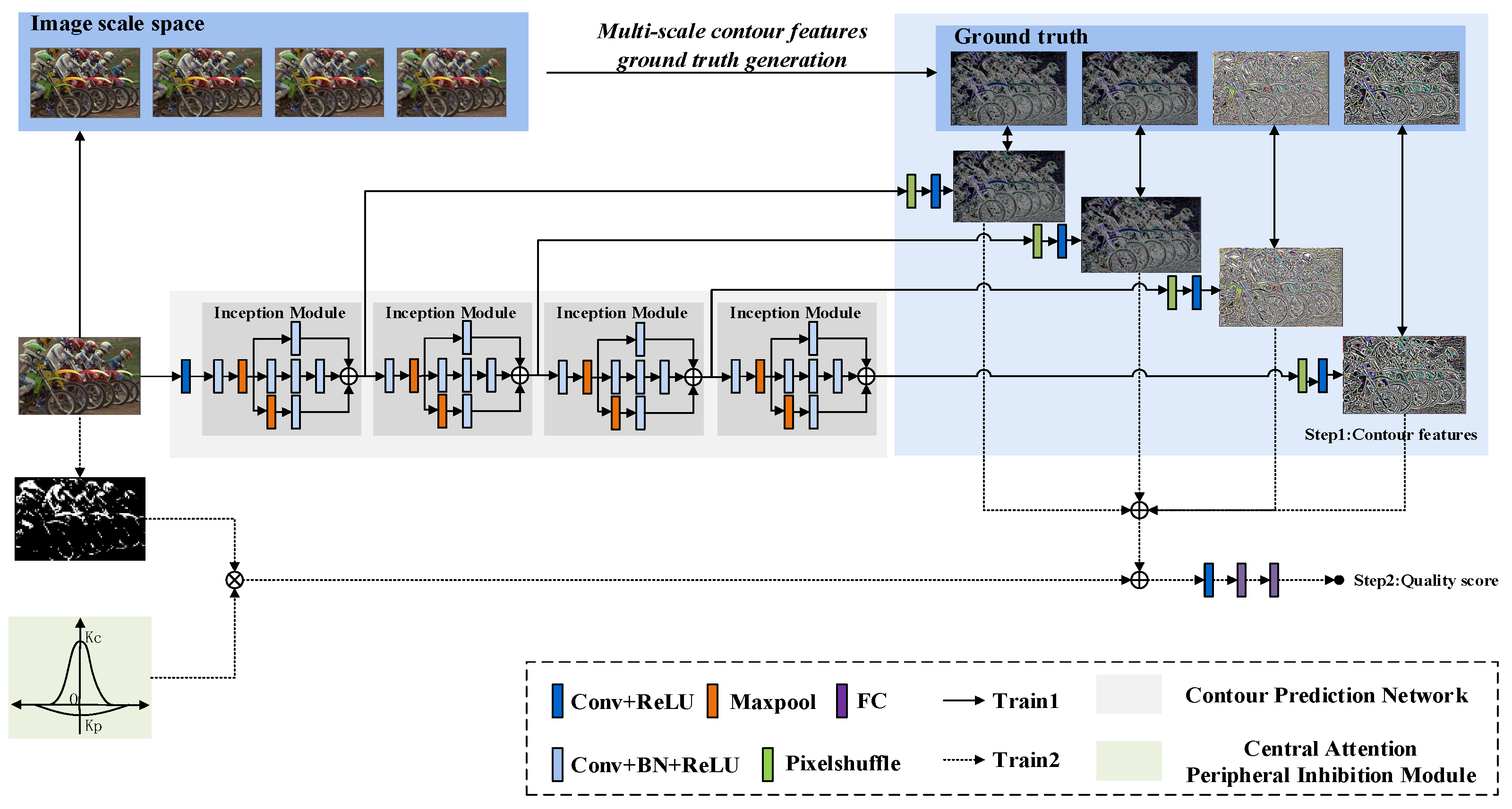
The overall framework of the MSIQA is shown in Figure 1. In the first stage of training, the multi-scale contour prediction network is trained to predict the contour features of diverse scale pictures in scale-spaces. In the second stage of training, the MSIQA model combines the central attention peripheral inhibition module to learn to predict the quality score of the image.

3.1. Model Architecture

The MSIQA model consists of two main modules: (1) a multi-scale contour prediction network to simulate the response of human eyes on an image’s contours at different distances, and (2) a central attention peripheral inhibition module to simulate the mechanism of the receptive field of retinal ganglion cells. We use four inception [31,32,33] modules with the same structure to build the contour prediction network. Each layer has a batch normalization (BN) [34] and a rectified linear unit (ReLU) [35]. After the inception module, the PixelShuffle [36] method is used to upscale the input feature to the same size as the input image. In the second stage of training, the outputs of different inception modules are first fused and combined with the central attention peripheral inhibition module, then fed into the convolutional layer and two fully connected layers.

3.2. Multi-Scale Contour Features

We believe that the sharpness of the edge contour of the image is an important feature that affects the image quality. At the same time, the same distortion type of the distorted images have different degrees of distortion, and the contour features of all images in the image scale space can simulate images with different degrees of distortion. Multi-scale features are used to simulate the contour response of the retina to images at different distances, so we train the model in the first stage to predict the contour features of images at different scales.

The scale-space of an image is the convolution of the image and the Gaussian function of the variable scale. The two-dimensional Gaussian function is:

$$G(x,y,\sigma )=\frac{1}{2\pi {\sigma }^2}\exp \left[-\frac{(x^2+y^2)}{2{\sigma }^2}\right]$$

(1)

The scale-space of an image $I(x,y)$ is:

$$L(x,y,{\sigma }_i)=\left\{I_0(x,y),I_1(x,y),\dots ,I_i(x,y)\right\}$$

(2)

where

$$I_i(x,y)=\{\begin{array}{c}I(x,y),i=0\\ G(x,y,{\sigma }_i)\ast I(x,y),i\ne 0\end{array}$$

(3)

The image subtraction of adjacent scales obtains the multi-scale contour features. Therefore, the contour feature ground truth is defined as:

$$\begin{array}{l}{D}_i(x,y)=I_i(x,y)-I_{i+1}(x,y)\\ =G(x,y,{\sigma }_i)\ast I(x,y)-G(x,y,{\sigma }_{i+1})\ast I(x,y)\\ =\left[G(x,y,{\sigma }_i)-G(x,y,{\sigma }_{i+1})\right]\ast I(x,y)\end{array}$$

(4)

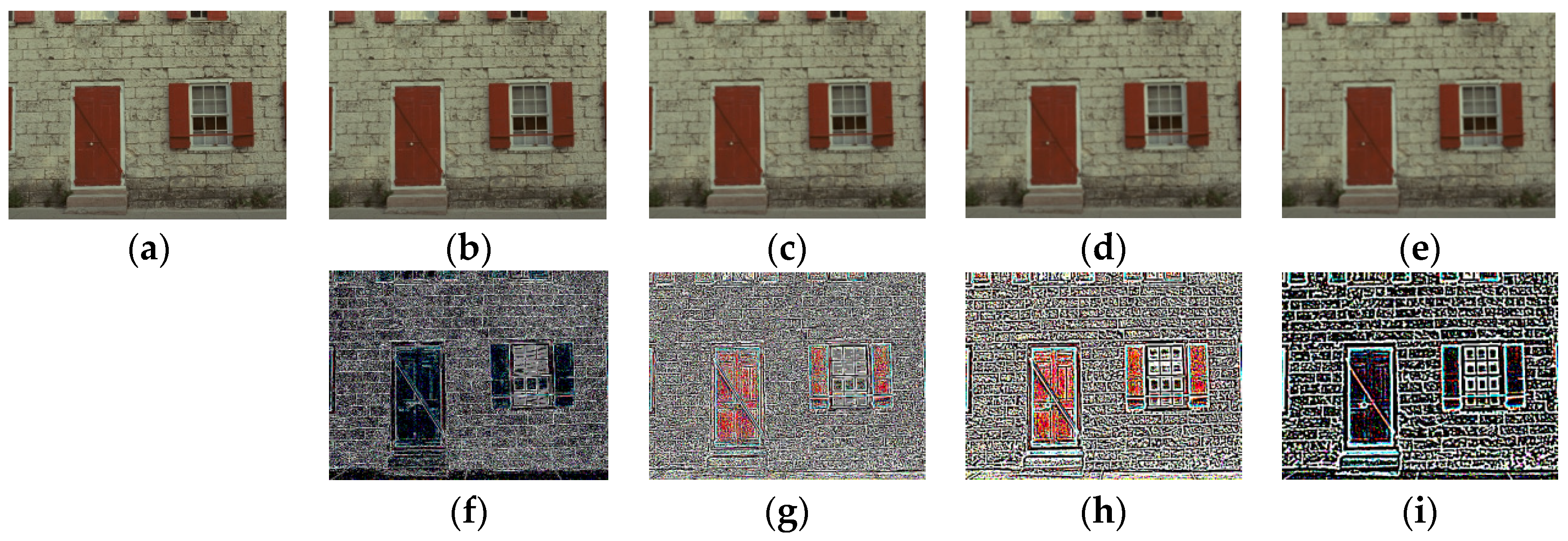
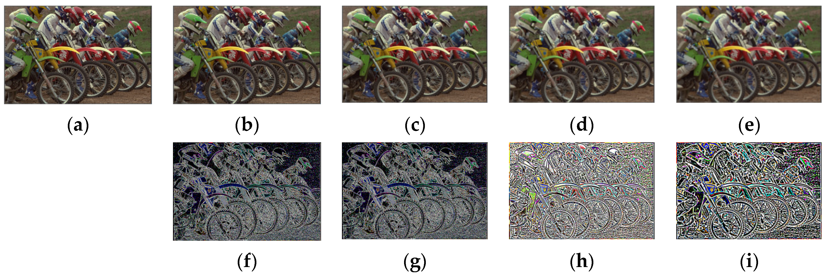
Figure 2 shows the generation of the multi-scale contour features ground truth. The images shown in Figure 3a–e are an image scale space of Figure 3a. The images shown in Figure 3f–i are contour features of different scales of the image in Figure 3a. Figure 4 is the same as Figure 3.

In the first stage of training, the contour prediction network learns to predict contour features, and the loss function is defined by the mean square error between the predicted value and the ground-truth:

$$L1=\frac{1}{N}{\displaystyle \sum _{i=1}^N{(D_i^m-h_{\theta }(I_i))}^2}$$

(5)

where $h_{\theta }(I_i)$ is the contour feature of the image $I_i$ predicted by the model, $\theta$ is the parameters of the contour prediction network, and $m$ is the exponent number. In our experiment, we choose $m=0.5$.

3.3. Quality Score Prediction

In the second step of training, the central attention peripheral inhibition module combines the brightness information of the image to weigh the multi-scale contour features learned in the first stage. The central attention peripheral inhibition module adopts a double Gaussian difference model, which is composed of two parts: the center position of the image has strong attention and the edge position is weakened, which simulates the different attention and different residence times of humans in different areas of the image. The distribution is:

$$S(x,y)=k_c\frac{1}{2\pi {\sigma }_c{}^2}\exp \left[-\frac{(x^2+y^2)}{2{\sigma }_c{}^2}\right]-k_p\frac{1}{2\pi {\sigma }_p{}^2}\exp \left[-\frac{(x^2+y^2)}{2{\sigma }_p{}^2}\right]$$

(6)

where $k_c$ is the central attention enhancement coefficient, $k_p$ is the peripheral inhibition coefficient.

Because the optic nerve has different sensitivity to images of different brightness, it is necessary to add brightness information of the image while considering the attention of different areas of the image. We normalized the overall image brightness and increased the quality score weight of image blocks with strong brightness.

The MSIQA model learns to predict image quality score. The loss function is defined as:

$$L2=\frac{1}{N}{\displaystyle \sum _{i=1}^N(S(I_i)-{h^{\prime }}_{\theta }(I_i))}$$

(7)

where ${h^{\prime }}_{\theta }(I_i)$ is the image quality score of the image $I_i$ predicted by the model, $\theta$ is the parameters of the CNN network, $S$ is the ground truth subjective score of the input image $I_i$.

3.4. Training

Because there are fully connected layers in the MSIQA model, the input size of the network must be unified. We have tested the effect of different sizes on the performance of the model, and the results are given in Section 4.

In the first stage of training, 80% of the images in the data set are randomly selected for training. First, the image is cropped into image patches of uniform size, and then the four-scale space images of each image patch are fed to the network for training. In the second stage of training, 80% of the images are randomly selected for training, and the image patches are directly fed to the network for training.

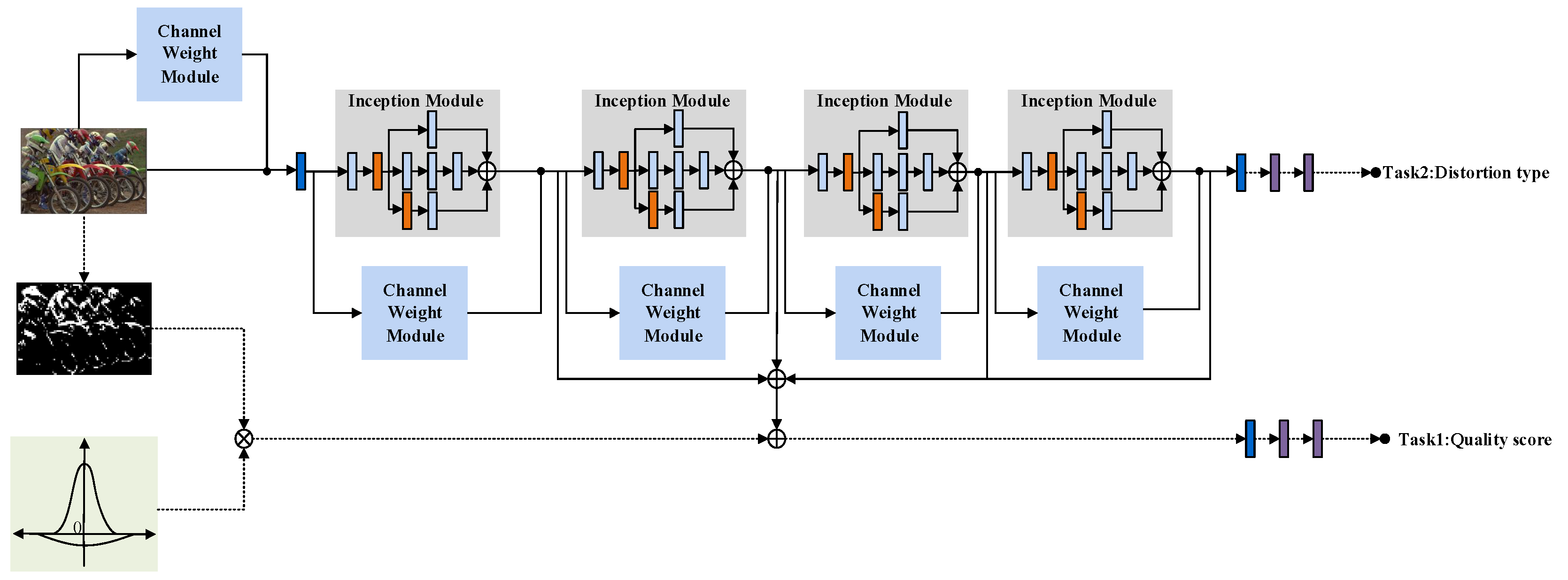
3.5. Multi-Task Model

Humans have various intuitive perceptions of different types of distortions. The types of distortions affect humans’ evaluation of image quality to a certain extent. Therefore, from the point of view of IQA, the detection of the distortion type is also of certain significance. At the same time, additional feature information of the distortion type is added to more strongly constrain the model and reduce the risk of overfitting.

The multi-task learning model adopts the hard parameter sharing method and adopts the basic structure of the MSIQA model proposed in 3.1. Task one is IQA, and task two is a classification of image distortion types. The overall framework of the model is shown in Figure 5.

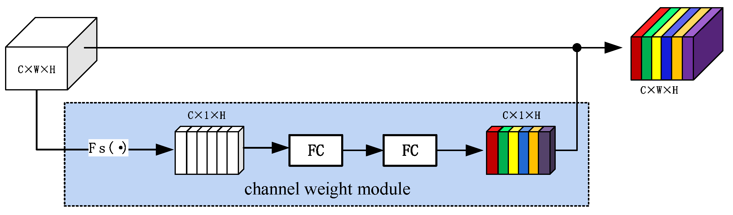
The image convolution operation can only obtain the relationship between local channels, and the network should learn important feature information from different feature channels. Referring to the idea proposed by Hu et al. [37], a feature channel weight module is added to the model, and the framework is shown in Figure 6.

First compress the input from size $C\times W\times H$ to $C\times 1\times H$:

$$Fs(x)=\frac{1}{W}{\displaystyle \sum _{i=1}^{W}x(i)}$$

(8)

where x is the input and W is the width of the input. After size compression, through two convolutional layers, the input channel weight is finally obtained, and then dot-multiply with input.

The loss weight of the two tasks adopts a dynamic weighting method. The loss function is defined as:

$$LOSS={\displaystyle \sum _{i=1}^2{\omega }_i(t)\ast L_i}$$

(9)

where $\omega$ is the weight of loss defined as:

$${\omega }_i(t)=\frac{2\exp (r_i(t)/T)}{{\displaystyle {\sum }_i\exp (r_i(t)/T)}},r_i(t)=\frac{L_i(t)}{L_i(t-1)}$$

(10)

where $L_i(t)$ is the loss of task $i$ in step $t$, $T$ is a constant.

4. Experiments and Analysis

4.1. Database and Evaluation Metrics

TID2013 and LIVE are the current mainstream databases for image quality evaluation. These databases provide the subjective score for each distorted image. The LIVE [23] database images are color images of different sizes, with 29 reference images, including five common types of distortion: additive white Gaussian noise (WN), Gaussian blur (GB), JPEG compression and JPEG2000 compression (JP2K) and fast-fading (FF). The image size of the TID2013 [24] database is 512 · 384, including 24 distortion types, each of which has five different degrees. The summary of each database is tabulated in

Table 1. Image distortion type.

TID2013	LIVE	Distortion Types
√	√	Additive Gaussian noise
√		Additive noise in color components
√		Spatially correlated noise
√		Masked noise
√		High-frequency noise
√		Impulse noise
√		Quantization noise
√	√	Gaussian blur
√		Image denoising
√	√	JPEG compression
√	√	JPEG2000 compression
√		JPEG transmission errors
√		JPEG2000 transmission errors
√		Non- eccentricity pattern noise
√		Local block-wise distortions of different intensity
√		Mean shift (intensity shift)
√		Contrast change
√		Change of color saturation
√		Multiplicative Gaussian noise
√		Comfort noise
√		Lossy compression of noisy images
√		Image color quantization with dither
√		Chromatic aberrations
√		Sparse sampling and reconstruction
	√	Fast-fading

[23,24].

The IQA algorithm performance depends on the correlation between the subjective score and the prediction score. If their correlation is high, it means that the performance of the algorithm is better. We used two standard measures, i.e., Spearman rank-order correlation coefficient (SRCC) and Pearson linear correlation coefficient (PLCC). The SRCC is defined as:

$$\mathrm{SRCC}=1-\frac{6{\displaystyle \sum _{i=1}^N{d}_i^2}}{N(N^2-1)}$$

(11)

where $d_i$ is the difference between the predicted score and ground-truth score of the $i\mathrm{th}$ image, and $N$ is the number of images. The PLCC is defined as:

$$\mathrm{PLCC}=\frac{{\displaystyle \sum _{\mathrm{i}=1}^N(p_i-\overline{p})(s_i-\overline{s})}}{\sqrt{{\displaystyle \sum _{\mathrm{i}=1}^N{(p_i-\overline{p})}^2}}\sqrt{{\displaystyle \sum _{\mathrm{i}=1}^N{(s_i-\overline{s})}^2}}}$$

(12)

where $p_i$ is the predicted score of the $i\mathrm{th}$ image, and $s_i$ is the ground-truth score of the $i\mathrm{th}$ image, $\overline{p}$ and $\overline{s}$ are the average of each.

4.2. Convergence Test

To validate the effect of the number of epochs in Step 1 on the performance in Step 2, we compared different training epochs in Step 1 (5, 10, 15 and 20) in the LIVE database shown in

Table 2. Comparison of the performance of step 2 with different training epochs in step 1.

Epoch Numbers in Step 1		5	10	15	20
Performance in step 2	SRCC	0.980	0.983	0.982	0.979
	PLCC	0.985	0.988	0.986	0.982

. For each test, the best is shown in bold. Therefore, 10 epochs were selected for Step 1.

4.3. Effect of Patch Size

In order to investigate the effect of patch size on the final prediction accuracy, we used four different patch sizes (64, 112, 224, and 384). As shown in

Table 3. Comparison of the SRCC and PLCC with different patch size.

Patch Size	64	112	224	384
SRCC	0.983	0.983	0.979	0.963
PLCC	0.988	0.988	0.985	0.968

, the patch size of 64 and 112 shows better performance in SRCC and PLCC. For each test, the best is shown in bold. Taking into account that when the patch size is too small, it is not conducive to the quality assessment of large-size images. Thus, a patch size of 112 was used in the following experiments.

4.4. Performances Comparison

We compared MSIQA with three FR-IQA methods (PSNR, SSIM [7], FSIMc [8]) and ten NR-IQA methods (BLINDS-II [9], BRISQUE [10], CORNIA [22], Kang [26], BIECON [14], Bosse [27], DeepBIQ [28], DIQA [15], Hallucinated [38], QualNet [39]). The test results of the MSIQA model on the LIVE data set and TID2013 data set are shown in

Table 4. Comparison of the SRCC and PLCC with different methods on LIVE and TID2013 database.

	Database	LIVE		TID2013
	Metrics	SRCC	PLCC	SRCC	PLCC
FR	PSNR	0.876	0.872	0.687	0.706
	SSIM	0.948	0.945	0.775	0.790
	FSIMc	0.963	0.960	0.851	0.877
NR	BLINDS-II	0.912	0.916	0.536	0.628
	BRISQUE	0.939	0.942	0.573	0.651
	CORNIA	0.942	0.943	0.549	0.613
	Kang	0.956	0.953	-	-
	BIECON	0.961	0.962	-	-
	Bosse	0.960	0.972	0.835	0.855
	DIQA	0.975	0.977	0.825	0.850
	Hallucinated	0.982	0.982	0.879	0.880
	QualNet	0.980	0.984	0.890	0.901
	MSIQA	0.983	0.988	0.877	0.880

. The test results of the MSIQA model for different distortion types in the LIVE data set are shown in

Table 5. Comparison of the SRCC with different methods on LIVE for different distortion types.

Type	PSNR	SSIM	FSIM	BRISQUE	CORNIA	BIECON	DIQA	MSIQA
JP2K	0.895	0.961	0.972	0.914	0.921	0.965	0.961	0.983
JPEG	0.881	0.972	0.979	0.965	0.938	0.987	0.976	0.984
WN	0.985	0.969	0.971	0.977	0.957	0.970	0.988	0.998
GB	0.782	0.952	0.968	0.951	0.957	0.945	0.962	0.980
FF	0.891	0.956	0.950	0.877	0.906	0931	0.912	0.972

. For each test, the best two models are shown in bold.

It can be seen from the results that our method performs very well on the LIVE dataset. The performance on the TID2013 dataset is not very good. We analyzed some images with large prediction errors and found that there are two reasons for this: (1) the TID2013 dataset contains non-real synthetic images, and the model is not designed with the images which synthetic and semantic information lacking. (2) Some of the distortion types in the TID2013 dataset are performed by changing the color of the image. Our model believes that in the case of no distortion of image details, such distortion types have little impact on the quality of the image, but have a greater impact on the aesthetic quality of the image. But the dataset is manually annotated, and humans give lower scores to images with unreasonable colors.

4.5. Multi-Task Model Test

We tested the IQA and distortion type classification of the multi-task model proposed by Section 3.5. Based on the MSIQA model, we trained the multi-task model. The test results in the case of very few training epochs (1–3) are shown in

Table 6. SRCC and PLCC and classification accuracy on LIVE and TID2013 databases.

Database	LIVE			TID2013
	SRCC	PLCC	Accuracy	SRCC	PLCC	Accuracy
MSIQA	0.983	0.988	-	0.877	0.880	-
MSIQA (multi-task)	0.988	0.996	0.846	0.879	0.881	0.811

. The joint tasks complement each other by sharing information, and even improve the performance of IQA. At the same time, we have made statistics on the classification accuracy of each distortion type, as shown in

Table 7. Distortion type classification accuracy on LIVE and TID2013 databases.

Database	JP2K	JPEG	WN	GB	FF
LIVE	0.987	0.760	0.833	0.846	0.836
TID2013	0.887	0.701	0.812	0.801	-

.

5. Conclusions

In this paper, we propose a biological vision-based multi-scale fusion NR-IQA model named MSIQA, which simulated the mechanism of the biological optic nerve and receptive field and adopts a two-stage training method. The MSIQA model fully combines the image contour feature, brightness and receptive field attention mechanism, and does not require reference images in the training and testing stages. As a result, the SRCC of the MSIQA model test on the LIVE database reached 0.983. On this basis, we propose a multi-task model that can classify distortion types at the same time. In the future, we will compress the model and increase the detection speed.

References

1. Zheng, H.; Sherazi, S.W.A.; Son, S.H.; Lee, J.Y. A Deep Convolutional Neural Network-Based Multi-Class Image Classification for Automatic Wafer Map Failure Recognition in Semiconductor Manufacturing. Appl. Sci. 2021, 11, 9769. [Google Scholar] [CrossRef]
2. Wang, F.; Ai, Y.; Zhang, W. Detection of Early Dangerous State in Deep Water of Indoor Swimming Pool Based on Surveillance Video. Signal Image Video Process. 2021, 16, 29–37. [Google Scholar] [CrossRef]
3. Chen, J.; Wang, F.; Li, C.; Zhang, Y.; Ai, Y.; Zhang, W. Online Multiple Object Tracking Using a Novel Discriminative Module for Autonomous Driving. Electronics 2021, 10, 2479. [Google Scholar] [CrossRef]
4. Jimenez, V.J.; Bouhmala, N.; Gausdal, A.H. Developing a Predictive Maintenance Model for Vessel Machinery. J. Ocean Eng. Sci. 2020, 5, 358–386. [Google Scholar] [CrossRef]
5. Zhou, T.; Wang, W.; Liang, Z.; Shen, J. Face Forensics in the Wild. In Proceedings of the 2021 IEEE/CVF Conference on Computer Vision and Pattern Recognition (CVPR), Nashville, TN, USA, 19–25 June 2021; pp. 5774–5784. [Google Scholar]
6. Adebayo, A.-A.; Atinuke, O.; Onashoga, S.; Misra, S.; Arogundade, O.; Abayomi-Alli, O. Facial Image Quality Assessment Using an Ensemble of Pre-Trained Deep Learning Models (EFQnet). In Proceedings of the 2020 20th International Conference on Computational Science and Its Applications (ICCSA), Cagliari, Italy, 1–4 July 2020; pp. 1–8. [Google Scholar]
7. Wang, Z.; Bovik, A.C.; Sheikh, H.R.; Simoncelli, E.P. Image Quality Assessment: From Error Visibility to Structural Similarity. IEEE Trans. Image Process. 2004, 13, 600–612. [Google Scholar] [CrossRef] [Green Version]
8. Lin, Z.; Lei, Z.; Mou, X.; Zhang, D. FSIM: A Feature Similarity Index for Image Quality Assessment. IEEE Trans. Image Process. 2011, 20, 2378–2386. [Google Scholar]
9. Saad, M.A.; Bovik, A.C.; Charrier, C. Blind Image Quality Assessment: A Natural Scene Statistics Approach in the DCT Domain. IEEE Trans. Image Process. 2012, 21, 3339–3352. [Google Scholar] [CrossRef] [PubMed]
10. Mittal, A.; Moorthy, A.K.; Bovik, A.C. No-Reference Image Quality Assessment in the Spatial Domain. IEEE Trans. Image Process. 2012, 21, 4695–4708. [Google Scholar] [CrossRef] [PubMed]
11. Wang, Z.; Simoncelli, E. Reduce-Reference Image Quality Assessment Using a Wavelet-Domain Natural Image Statistic Model. In Proceedings of the SPIE Elecronic Imaging Conference, San Jose, CA, USA, 16–20 January 2005; Volume 5666. [Google Scholar] [CrossRef] [Green Version]
12. Soundararajan, R.; Bovik, A.C. RRED Indices: Reduced Reference Entropic Differencing for Image Quality Assessment. IEEE Trans. Image Process. 2012, 21, 517–526. [Google Scholar] [CrossRef] [Green Version]
13. Wei, L.; Zhao, L.; Peng, J. Reduced Reference Quality Assessment for Image Retargeting by Earth Mover’s Distance. Appl. Sci. 2021, 11, 9776. [Google Scholar] [CrossRef]
14. Kim, J.; Lee, S. Fully Deep Blind Image Quality Predictor. IEEE J. Sel. Top. Signal Process. 2017, 11, 206–220. [Google Scholar] [CrossRef]
15. Kim, J.; Nguyen, A.-D.; Lee, S. Deep CNN-Based Blind Image Quality Predictor. IEEE Trans. Neural Netw. Learn. Syst. 2019, 30, 11–24. [Google Scholar] [CrossRef] [PubMed]
16. Moorthy, A.K.; Bovik, A.C. A Two-Step Framework for Constructing Blind Image Quality Indices. IEEE Signal Process. Lett. 2010, 17, 513–516. [Google Scholar] [CrossRef]
17. Xue, W.; Mou, X.; Zhang, L.; Bovik, A.C.; Feng, X. Blind Image Quality Assessment Using Joint Statistics of Gradient Magnitude and Laplacian Features. IEEE Trans. Image Process. 2014, 23, 4850–4862. [Google Scholar] [CrossRef]
18. Zhang, L.; Zhang, L.; Bovik, A.C. A Feature-Enriched Completely Blind Image Quality Evaluator. IEEE Trans. Image Process. 2015, 24, 2579–2591. [Google Scholar] [CrossRef] [Green Version]
19. Wu, Q.; Wang, Z.; Li, H. A Highly Efficient Method for Blind Image Quality Assessment. In Proceedings of the 2015 IEEE International Conference on Image Processing (ICIP), Quebec, QC, Canada, 27–30 September 2015; pp. 339–343. [Google Scholar]
20. Wu, Q.; Li, H.; Meng, F.; Ngan, K.N.; Luo, B.; Huang, C.; Zeng, B. Blind Image Quality Assessment Based on Multichannel Feature Fusion and Label Transfer. IEEE Trans. Circuits Syst. Video Technol. 2016, 26, 425–440. [Google Scholar] [CrossRef]
21. Mittal, A.; Soundararajan, R.; Bovik, A.C. Making a “Completely Blind” Image Quality Analyzer. IEEE Signal Process. Lett. 2013, 20, 209–212. [Google Scholar] [CrossRef]
22. Ye, P.; Kumar, J.; Kang, L.; Doermann, D. Unsupervised Feature Learning Framework for No-Reference Image Quality Assessment. In Proceedings of the 2012 IEEE Conference on Computer Vision and Pattern Recognition, Providence, RI, USA, 16–21 June 2012; pp. 1098–1105. [Google Scholar]
23. Sheikh, H.R. LIVE Image Quality Assessment Database. 2003. Available online: http://live.ece.utexas.edu/research/quality (accessed on 4 April 2021).
24. Ponomarenko, N.; Jin, L.; Ieremeiev, O.; Lukin, V.; Egiazarian, K.; Astola, J.; Vozel, B.; Chehdi, K.; Carli, M.; Battisti, F.; et al. Image Database TID2013: Peculiarities, Results and Perspectives. Signal Process. Image Commun. 2015, 30, 57–77. [Google Scholar] [CrossRef] [Green Version]
25. Kim, J.; Zeng, H.; Ghadiyaram, D.; Lee, S.; Zhang, L.; Bovik, A.C. Deep Convolutional Neural Models for Picture-Quality Prediction: Challenges and Solutions to Data-Driven Image Quality Assessment. IEEE Signal Process. Mag. 2017, 34, 130–141. [Google Scholar] [CrossRef]
26. Le, K.; Peng, Y.; Yi, L.; Doermann, D. Convolutional Neural Networks for No-Reference Image Quality Assessment. In Proceedings of the 2014 IEEE Conference on Computer Vision and Pattern Recognition, Columbus, OH, USA, 23–28 June 2014; pp. 1733–1740. [Google Scholar]
27. Bosse, S.; Maniry, D.; Muller, K.-R.; Wiegand, T.; Samek, W. Deep Neural Networks for No-Reference and Full-Reference. IEEE Trans. Image Process. 2018, 27, 206–219. [Google Scholar] [CrossRef] [Green Version]
28. Bianco, S.; Celona, L.; Napoletano, P.; Schettini, R. On the Use of Deep Learning for Blind Image Quality Assessment. Signal Image Video Process. 2018, 12, 355–362. [Google Scholar] [CrossRef]
29. Liu, X.; Weijer, J.; Bagdanov, A.D. RankIQA: Learning from Rankings for No-Reference Image Quality Assessment. In Proceedings of the 2017 IEEE International Conference on Computer Vision (ICCV), Venice, Italy, 22–29 October 2017; pp. 1040–1049. [Google Scholar]
30. Talebi, H.; Milanfar, P. NIMA: Neural Image Assessment. IEEE Trans. Image Process. 2018, 27, 3998–4011. [Google Scholar] [CrossRef] [PubMed] [Green Version]
31. Szegedy, C.; Liu, W.; Jia, Y.; Sermanet, P.; Reed, S.; Anguelov, D.; Erhan, D.; Vanhoucke, V.; Rabinovich, A. Going Deeper with Convolutions. In Proceedings of the 2015 IEEE Conference on Computer Vision and Pattern Recognition (CVPR), Boston, MA, USA, 7–12 June 2015; pp. 1–9. [Google Scholar]
32. Szegedy, C.; Vanhoucke, V.; Ioffe, S.; Shlens, J.; Wojna, Z. Rethinking the Inception Architecture for Computer Vision. In Proceedings of the 2016 IEEE Conference on Computer Vision and Pattern Recognition (CVPR), Las Vegas, NV, USA, 17–30 June 2016; pp. 2818–2826. [Google Scholar]
33. Szegedy, C.; Ioffe, S.; Vanhoucke, V.; Alemi, A. Inception-v4, Inception-ResNet and the Impact of Residual Connections on Learning. arXiv 2016, arXiv:1602.07261. [Google Scholar]
34. Ioffe, S.; Szegedy, C. Batch Normalization: Accelerating Deep Network Training by Reducing Internal Covariate Shift. arXiv 2015, arXiv:1502.03167. [Google Scholar]
35. Nair, V.; Hinton, G.E. Rectified Linear Units Improve Restricted Boltzmann Machines. In Proceedings of the 27th International Conference on International Conference on Machine Learning, Haifa, Israel, 21–24 June 2010; pp. 807–814. [Google Scholar]
36. Shi, W.; Caballero, J.; Huszár, F.; Totz, J.; Aitken, A.P.; Bishop, R.; Rueckert, D.; Wang, Z. PixelShuffle: Real-Time Single Image and Video Super-Resolution Using an Efficient Sub-Pixel Convolutional Neural Network. In Proceedings of the IEEE Conference on Computer Vision and Pattern Recognition (CVPR), San Francisco, CA, USA, 18–20 June 2016; pp. 1874–1883. [Google Scholar]
37. Hu, J.; Shen, L.; Albanie, S.; Sun, G.; Wu, E. Squeeze-and-Excitation Networks. IEEE Trans. Pattern Anal. Mach. Intell. 2020, 42, 2011–2023. [Google Scholar] [CrossRef] [Green Version]
38. Lin, K.; Wang, G. Hallucinated-IQA: No-Reference Image Quality Assessment via Adversarial Learning. In Proceedings of the 2018 IEEE/CVF Conference on Computer Vision and Pattern Recognition, Salt Lake City, UT, USA, 18–23 June 2018; pp. 732–741. [Google Scholar]
39. Golestaneh, S.A.; Kitani, K. No-Reference Image Quality Assessment via Feature Fusion and Multi-Task Learning. arXiv 2020, arXiv:2006.03783. [Google Scholar]
Figure 1. Illustration of the MSIQA model. The model consists of a multi-scale Contour Prediction Network and a Central Attention Peripheral Inhibition Module. The solid line is the first step of training, and the dashed line is the second step of training.
Applsci 12 02833 g001
Figure 2. The generation of the multi-scale contour features.
Applsci 12 02833 g002
Figure 3. Examples of scale space and contour features of a image in the TID2013 database. (a)–(e) are an image scale space of (a). (f)–(i) are contour features of different scales of (a).
Applsci 12 02833 g003
Figure 4. Examples of scale space and contour features of a image in the LIVE database. (a)–(e) are an image scale space of (a). (f)–(i) are contour features of different scales of (a).
Applsci 12 02833 g004
Figure 5. The overall framework of the model.
Applsci 12 02833 g005
Figure 6. The framework of channel weight module.
Applsci 12 02833 g006