Article

Calculation of View Factors for Building Simulations with an Open-Source Raytracing Tool

1
Department of Civil Engineering, TU Kaiserslautern, 67663 Kaiserslautern, Germany
2
Department of Mechanical Engineering, Coimbatore Institute of Technology, Coimbatore 641014, India
3
Anyhere Software, Berkeley, CA 94708, USA
*
Author to whom correspondence should be addressed.
Appl. Sci. 2022, 12(6), 2768; https://doi.org/10.3390/app12062768
Submission received: 18 January 2022 / Revised: 24 February 2022 / Accepted: 4 March 2022 / Published: 8 March 2022
(This article belongs to the Special Issue Heat Transfer in Buildings)

Abstract

:
Longwave radiative heat transfer is a key determinant of energy consumption in buildings and view factor calculations are therefore required for the detailed simulation of heat transfer between buildings and their environment as well as for heat exchange within rooms. Typically, these calculations are either derived through analytical means or performed as a part of the simulation process. This paper describes the methodology for employing RADIANCE, a command-line open-source raytracing software, for performing view factor calculations. Since it was introduced in the late-1980s, RADIANCE has been almost exclusively employed as the back-end engine for lighting simulations. We discuss the theoretical basis for calculating view factors through Monte Carlo calculations with RADIANCE and propose a corresponding workflow. The results generated through RADIANCE are validated by comparing them with analytical solutions. The fundamental methodology proposed in this paper can be scaled up to calculate view factors for more complex, practical scenarios. Furthermore, the portability, multi-processing functionality and cross-platform compatibility offered by RADIANCE can also be employed in the calculation of view factors.

1. Introduction

Longwave radiative heat transfer is a key determinant of energy consumption in buildings. The radiative heat exchange between the outer surfaces of the building envelope and the surroundings account for a significant portion of the overall heat loss of a building, e.g., under clear sky conditions during night time. Additionally, the longwave radiative processes in rooms when, e.g., using radiant cooling or heating, influence the temperature distribution on floor, walls, and ceiling.
Radiant heat exchange between two surfaces is a function of their relative orientation and distance from one another, surface properties and absolute temperatures. The effect of relative orientation and spacing on radiant heat exchange between two surfaces can be quantified by a purely geometric parameter called view factor [1]. The knowledge of view factors is required whenever the longwave radiative heat transfer of building surfaces needs to be calculated in detail.
Analyses such as energy simulations, photovoltaic simulations, lighting simulations and thermal comfort simulations employ view factor calculations to assess the radiative exchange between surfaces of buildings, urban contexts, and the human body. Additionally, view factors are also required in the design of several engineering applications like satellite temperature control devices, solar collectors, advanced engines with high operating temperatures, and cryogenic fuel storage tanks [2].
View factor is independent of surface properties and temperatures, and is also referred to as shape factor, configuration factor, or angle factor. View factors calculated by assuming surfaces to be either diffuse emitters or diffuse reflectors are known as diffuse view factors. In this paper, the term view factor is intended to imply diffuse view factors. For two arbitrarily oriented surfaces A 1 and A 2 in space as shown in Figure 1, assuming the surfaces to be of equal radiance, the view factor F12 from A 1 to A 2 is the fraction of radiation leaving surface one that reaches surface two directly [1]. Likewise, the view factor F21 is the fraction of radiation leaving surface two that reaches surface one directly.
In this paper, the term “radiance” when used with proper capitalization (as “radiance” or “Radiance”), refers to the radiant flux per unit solid angle per unit projected area (W/(sr*m2)). In instances where the term is capitalized in uppercase as “RADIANCE”, it refers to the raytracing software that will be discussed in the subsequent sections.
A generalized expression for F12 can be derived by considering differential surface elements d A 1 and d A 2 on A 1 and A 2 respectively. For the two area elements, the view factor is:
F d A 1 d A 2 = cos θ 1 cos θ 2 π r 2 d A 2  
where r is the distance between dA1 and dA2, θ1 is the angle between the surface-normal of dA1 and the line connecting dA1 and dA2, and θ2 is the angle between the surface-normal of dA2 and the line connecting dA1 and dA2. The view factor between dA1 and the entire area A2 can be calculated as:
F d A 1 A 2 = A 2 cos θ 1 cos θ 2 π r 2 d A 2      
View factors between two finite areas A1 and A2 obey the following relation:
A 1 F 12 = A 1 A 2 cos θ 1 cos θ 2 π r 2 d A 2 d A 1 = A 2 F 21
Computational algorithms specifically addressed towards view factor calculations have existed for over seven decades [3]. Such algorithms employ either analytical or probabilistic techniques, broadly referred to as Radiosity and Monte Carlo methods, respectively [4]. Prominent radiosity-based methods include the hemisphere method [5], the hemicube method [6] and adaptive integration [7]. Different implementations of the Monte Carlo method have been proposed since the 1960s. One of earliest applications of Monte Carlo method to heat transfer was proposed by Howell in 1969 [8], wherein the possibility of applying this method to calculations with complex surfaces and simultaneous effects was discussed in the context of computing systems. In the subsequent years, several applications and optimizations around this method have been proposed by numerous studies. For example, a triangular subdivision approach to handle occluded surfaces was proposed by Hien and Chirarattananon in 2005 [9]. Vujicic et al. evaluated the impact of discretization of surfaces through meshing to improve the accuracy of simulations [10]. Recent studies also focus on the applicability of Monte Carlo method for specific use-cases, such as the one by Mirhosseini and Saboonchi (2011) to calculate the view factor between a 3D strip element to a circular cylinder [11]. Fei et al. (2018) discuss the effectiveness of the Monte Carlo method for calculating view factors for several complex surfaces such as torus, parallel cylinders and radiant tubes in annealing furnaces [12].
Several tools have been developed specifically for the purposes of calculating view factors. Among these View3D [7] and VISRAD [13] employ Radiosity-based approach and Mont3D [14] employs the Monte Carlo method. Presently, none of these tools are under active development and therefore have not been optimized to leverage the features such as multi-processing, cloud-computing and GPU-based calculations that are present in modern computing systems. Additionally, such tools are not particularly suited for calculations with complex shapes that involve multiple obstructions and curvatures [7]. Building simulation tools that perform view factor calculations, usually through the Radiosity approach, do so as a part of their overall workflow, and do not offer specific functionality to calculate view factors alone.
This paper introduces the application of RADIANCE, a raytracing tool used primarily for lighting simulations, to calculate view factors. RADIANCE differs from the previously mentioned view factor calculation tools in several aspects. It has been under continuous development for the past three decades and can leverage the advance features offered by modern computing systems. It also supports complex shapes and obstructions. In the following sections we introduce this tool and discuss its view factor calculation methodology.

2. RADIANCE: Theoretical Basis and General Calculation Methodology

2.1. Introduction and Background

RADIANCE is a collection of over a hundred independent command-line programs that are invoked in customized sequences to perform different types of lighting and daylighting simulations. It was developed in the mid-1980s at the Lawrence Berkeley National Laboratory by Greg Ward and has been under continued development since then. Detailed documentation about Radiance and its application for lighting and daylighting simulations can be found on https://www.radiance-online.org/ (accessed on 6 March 2022). The source code of Radiance and the compiled executables for different platforms are hosted at https://github.com/LBNL-ETA/Radiance (accessed on 6 March 2022). Initial research on RADIANCE focused on the development of its raytracing methodology [15] to simulate illuminated spaces [16]. The functionality of RADIANCE to accurately calculate photopic luminance [17] and a discussion on the underlying algorithms [18] can be found in the papers published by Ward in the late 1980s.The results for lighting and daylighting simulations generated through RADIANCE have been empirically validated by an extensive body of research in the past three decades. An empirical validation of RADIANCE for simulating artificially lit spaces was conducted by Grynberg in 1989 [19] and corresponding validation for daylit spaces was published by Mardaljevic in 1995 [20]. Validation studies undertaken in the past decade have involved the use of complex shading systems [21] and annual daylighting simulation methods [22].
A schematic diagram showing the standard inputs and workflow for RADIANCE is shown in Figure 2. As is evident from the figure, the simulation methodology features the invocation of multiple programs in a specific sequence [23].
The core application of RADIANCE relates to raytracing. The purpose of the raytracing is to recursively evaluate Equation (4) at every sampled surface point of the geometry.
L r θ r , φ r = L e θ e , φ e + φ = 0 2 π θ = 0 π / 2 L i θ i , φ i ρ b d θ i , φ i ; θ r , φ r   cos θ i sin θ i d θ i d φ i
where θ is the polar angle measured from the surface normal, φ is the azimuthal angle, Le(θe, φe) is the emitted radiance in W/(sr*m2), Lr(θr, φr) is the reflected radiance, Li(θi, φi) is the incident radiance and ρbd(θi, φi, θr, φr) is the bidirectional reflectance-transmittance distribution function in sr−1. As indicated by the terms Le, Lr, and Li in Equation (4), the raytracing process calculates radiant energy emitted, reflected, and incident (respectively) at every sampled surface point.
The raytracing algorithms are primarily accessed through three programs, namely: rtrace, rpict, and rcontrib. The surface-sampling methodology implemented in these programs is a combination of deterministic and stochastic sampling. In the context of lighting and daylighting simulations, deterministic sampling is used for calculating the radiant energy emitted by direct radiation sources like the sun or light fixtures. Stochastic sampling, which employs the Monte Carlo method, is used to calculate emitted or reflected radiation from diffuse sources like building surfaces. While rpict and rtrace incorporate additional techniques like ambient caching that are computationally efficient for lighting and daylighting applications, rcontrib employs a pure Monte Carlo approach. Rcontrib has so far been used, and validated, for calculating irradiance (W/m2) and radiance (W/(sr*m2)) values for annual daylighting simulations [24]. In the following section, we discuss the functionality, theoretical basis and syntax of rcontrib, and propose how it can be used to calculate view factors.

2.2. Calculating View Factors

As per its user-manual, rcontrib computes “contribution coefficients in a RADIANCE scene” [25]. The term “scene” collectively refers to the geometry and material properties of all the surfaces that are being considered in the calculation. Assuming every surface in the scene to be of equal radiance, at any point in the scene the “contribution coefficient” from a particular surface relates to the fraction of radiant energy received from it.
Rcontrib permits the calculation of both radiance and irradiance coefficients through different input parameters. As documented in [25], these coefficients typically relate to radiant flux transfer between sky and ground or optical systems such as light pipes and shading systems. The specificity of input parameters in each instance depends on the type of coefficient, material properties of the surfaces and the complexity of geometry.
To calculate view factors, a hitherto undocumented application, rcontrib needs to be invoked in the irradiance (-I) mode with a single ambient bounce (-ab 1). The resultant direct “contribution coefficient” of a finite distant surface A1 at a given differential surface dA1 is its view factor multiplied by π. This is syntactically expressed and illustrated in Figure 3.
As shown in Figure 3a, the differential surface dA1 is specified by the cartesian coordinates (x1, y1, z1) and direction vector (vx1, vy1, vz1). The green dots on the surface indicate Monte Carlo sampling which is controlled by the parameter N for ambient divisions (-ad) and limit weight (-lw) as shown in Figure 3b. The parameter for ambient bounces needs to be retained to its default value of one to ensure that no diffuse interreflection between surfaces is considered. For standard rcontrib simulations relating to electric lights and daylight, the ambient bounces are usually set to four and higher.
The syntax for the command is shown in Figure 3c. The process of calculating view factors can be explained in the following steps:
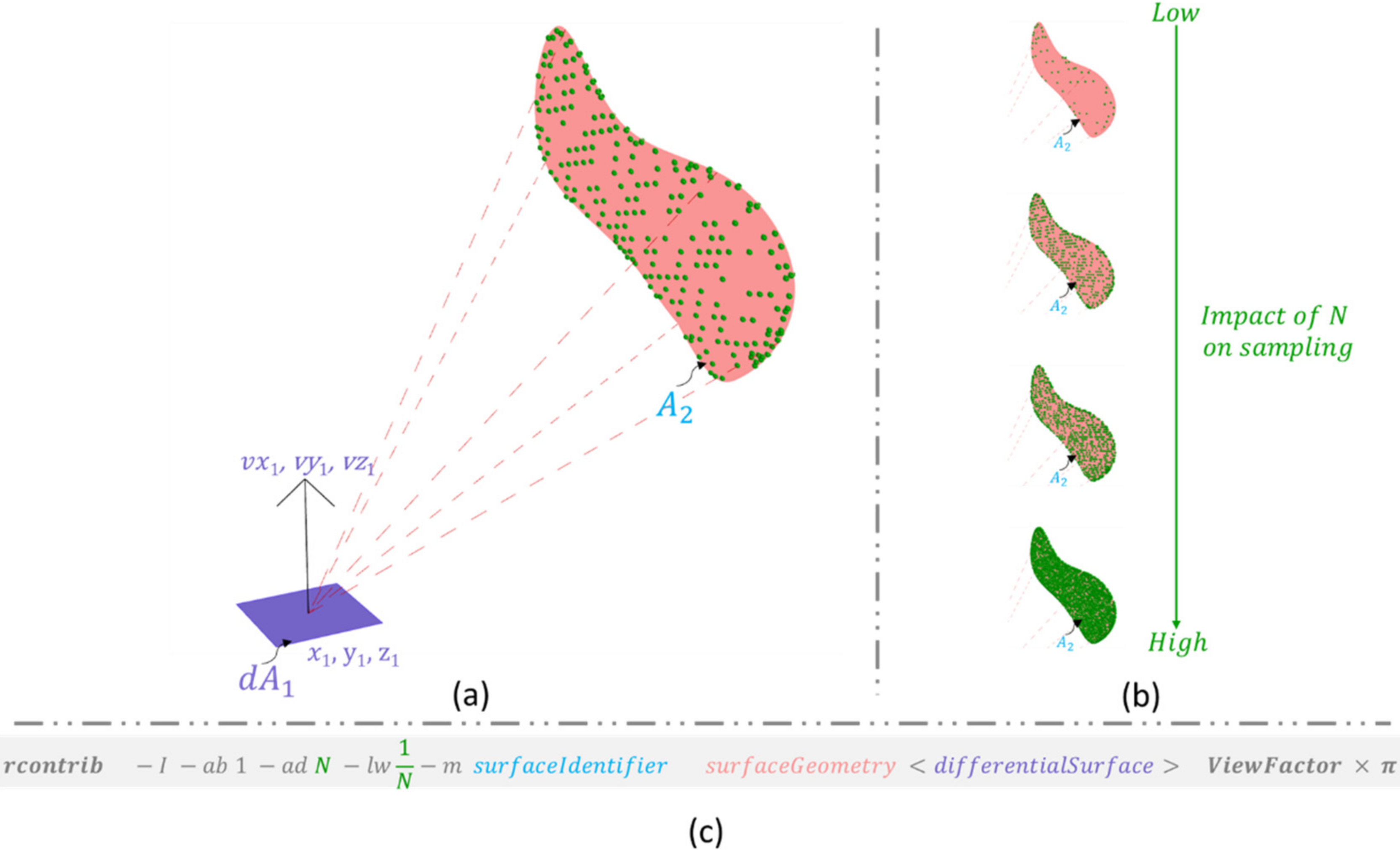
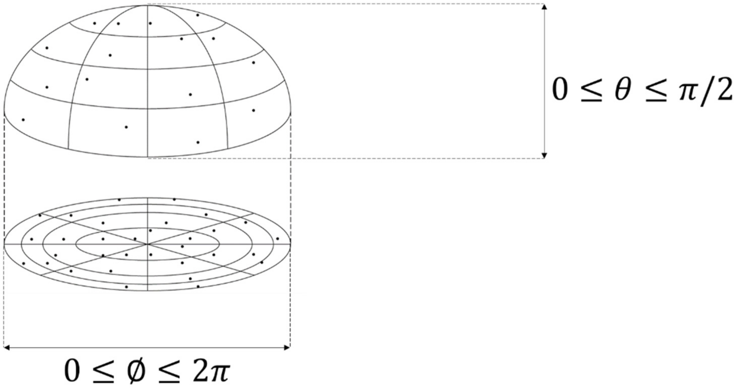
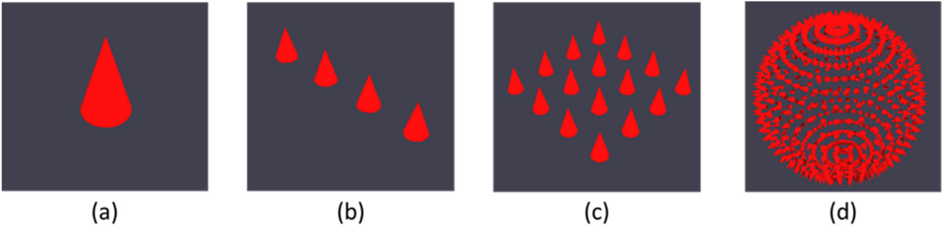
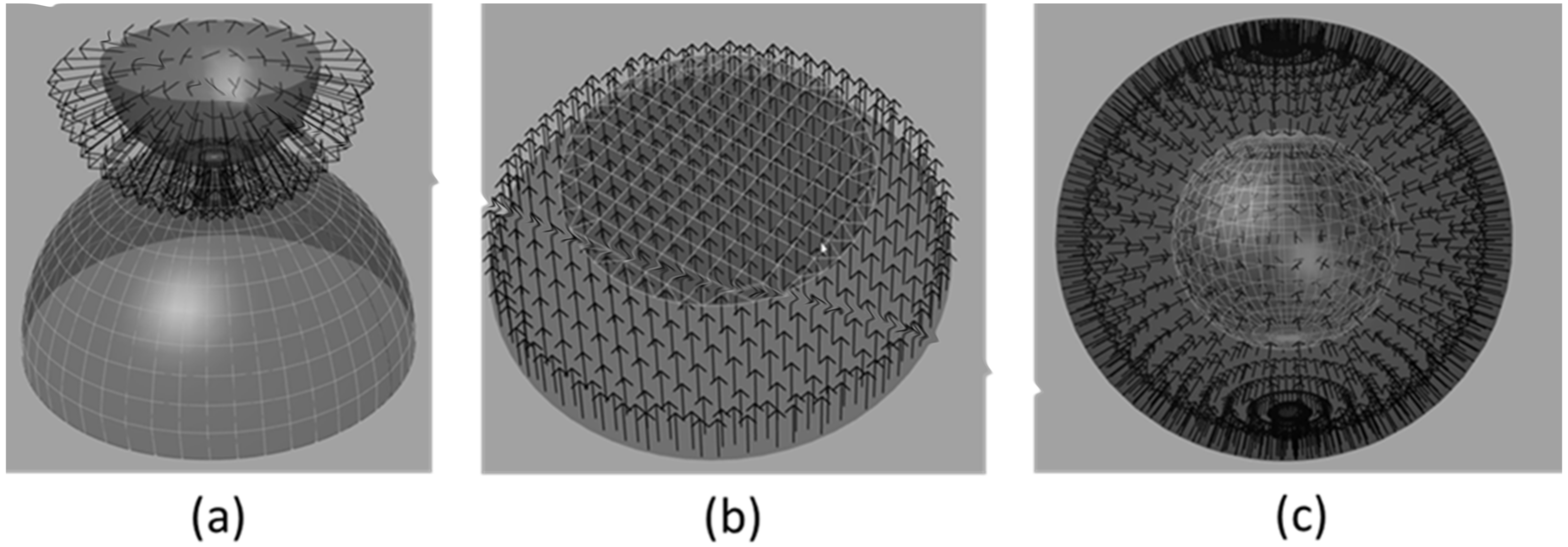
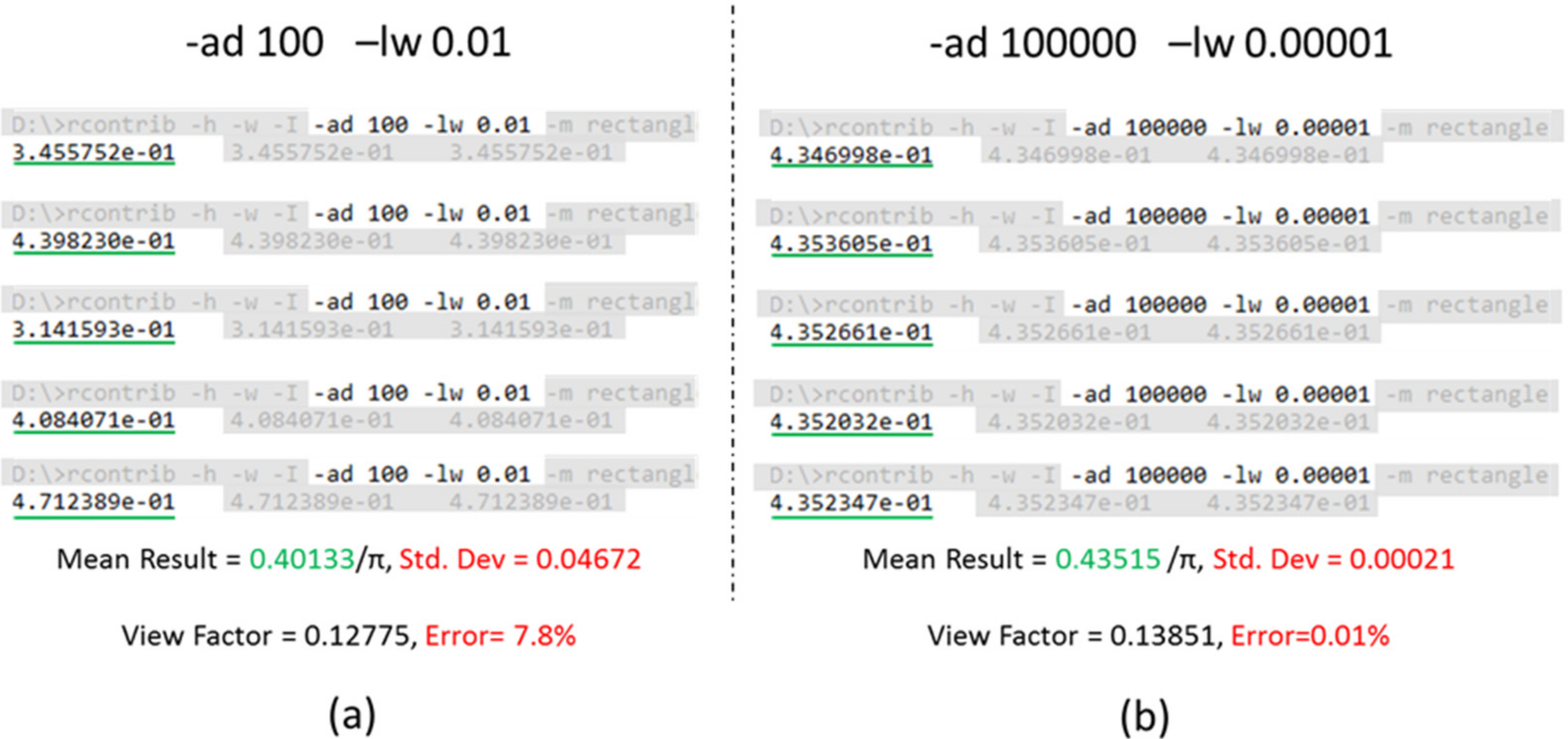
  • For a given infinitesimal area dA1, N rays are stochastically mapped over a hemispherical basis as shown in Figure 4. The approach for randomly mapping these rays is based on the methodology proposed by Shirley and Chiu [26]. For the random sampling to converge, such that the results from two independent ray tracing processes are numerically within a tolerance range of less than 1%, a large number of samples is required.
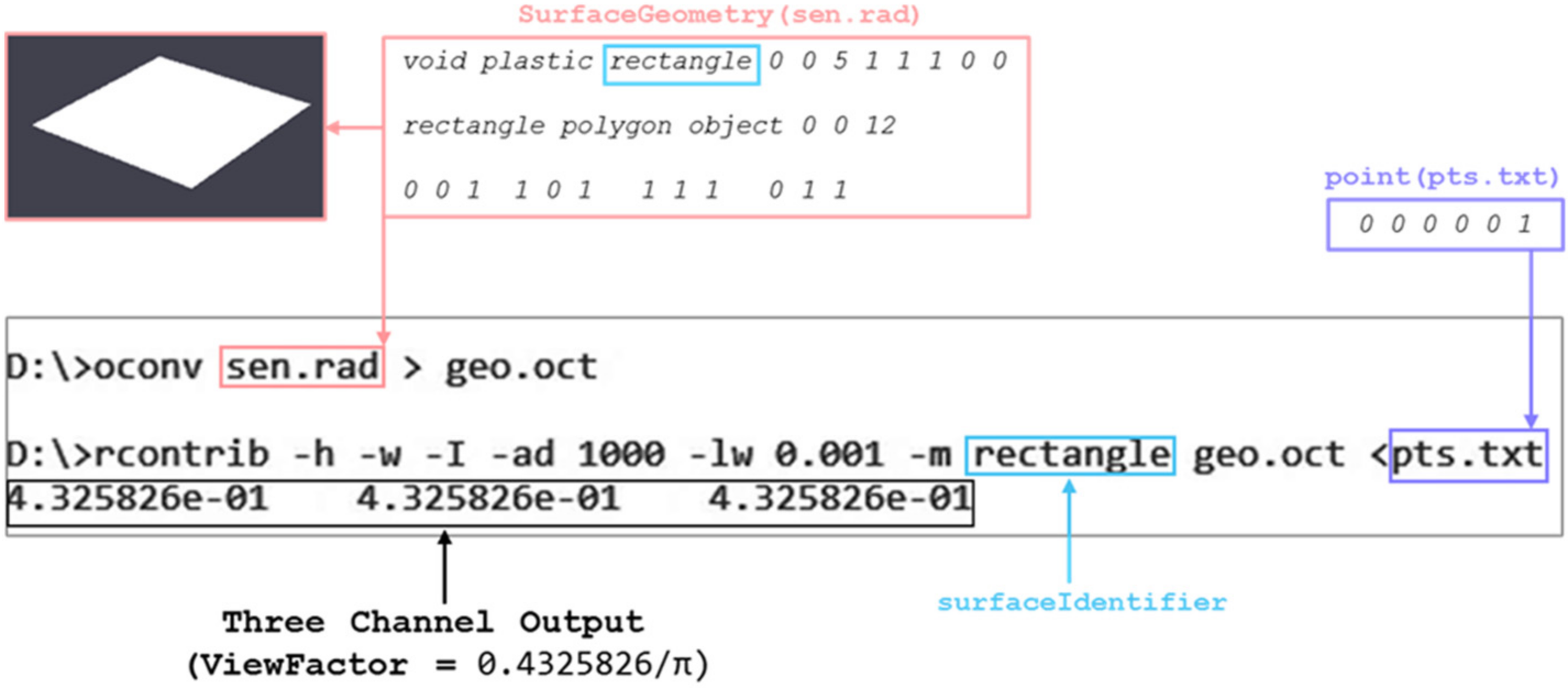
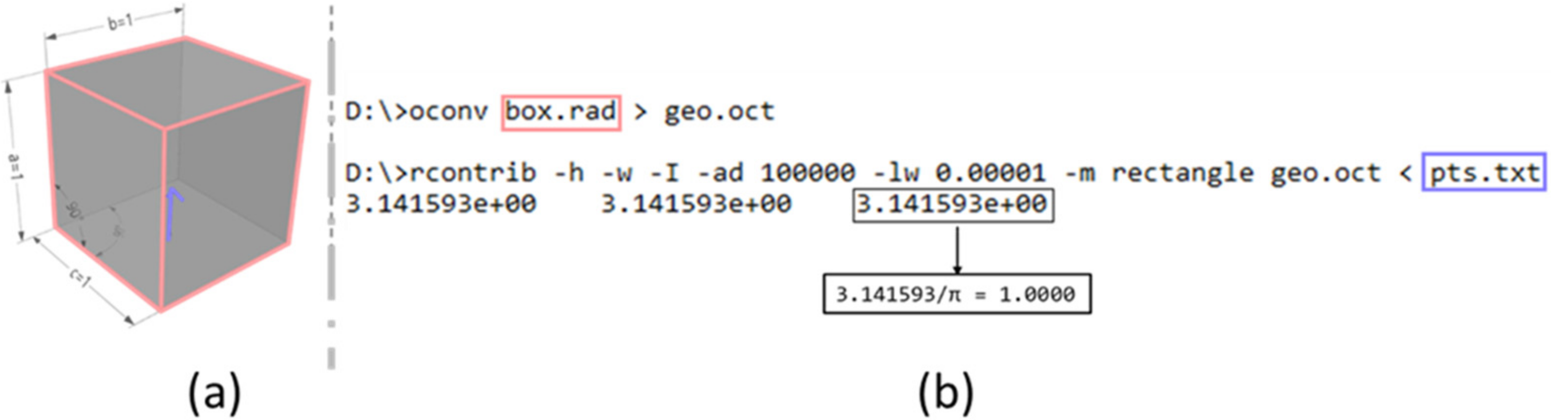
  • For each ray that strikes the geometry of the surface(s) identified through “surfaceIdentifier”, a contribution is added. The contribution of a single ray will be equal to π/N, where the presence of the value of π is owing to the use of irradiance integral.
  • The sum of all ray contributions to the surface identified through the surface identifier constitutes the fraction of the total hemispherical basis viewed by the infinitesimal area. This fraction constitutes an approximation of the view factor. As explained through Figure 3c, the output generated through RADIANCE is the approximate view factor multiplied by a factor of π.
The process outlined in the above steps is the basis of all view factor calculations discussed in this paper. The mathematical basis for this calculation can be expressed by Equation (5), where the term E i n d denotes indirect-irradiance. The other terms have the same interpretation as in Equation (4).
E i n d θ i , φ i = φ = 0 2 π θ = 0 π / 2 L i θ i , φ i   cos θ i sin θ i d θ i d φ i
As indicated by Figure 3b, the amount of stochastic sampling of a particular surface is controllable by increasing or decreasing N, the value for the ambient divisions (-ad) parameter, which in turn necessitates decreasing or increasing the limit weight (-lw) parameter respectively. Ambient divisions directly control the number of rays used for sampling and limit weight controls the contribution of each ray to the final result. So, the value of 1/N for limit weight indicates that each ray is given equal weightage. As is expected of any Monte Carlo raytracing method, higher sampling leads to a better estimation of the result.
Based on the illustrations in Figure 3, the functionality and methodology for calculation of view factors can be broadly communicated in simple terms. However, the specific inputs provided to rcontrib need to be in a format that is compatible with RADIANCE and the outputs received from rcontrib need to be post-processed to derive the actual view factor. Accordingly, the invocation of rcontrib is preceded and followed by a sequence of steps that is shown in Figure 5.
Figure 5 introduces an additional RADIANCE program called oconv. Oconv creates an octree data-structure that facilitates efficient raytracing by reducing the number of ray-surface intersections [27]. The octree data-structure is a pre-requisite for all the raytracing programs in RADIANCE [28]. The “post-processing” box shown in the figure relates to extracting the results from rcontrib, dividing the results by π as described earlier and finally performing case-appropriate view factor algebra operations. The methodology for specifying inputs, and deriving view factors from outputs, is explained in the following section.

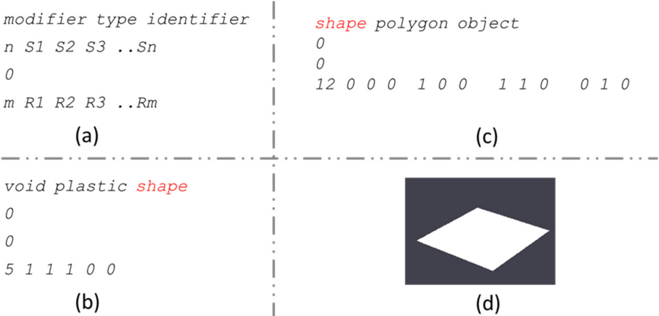
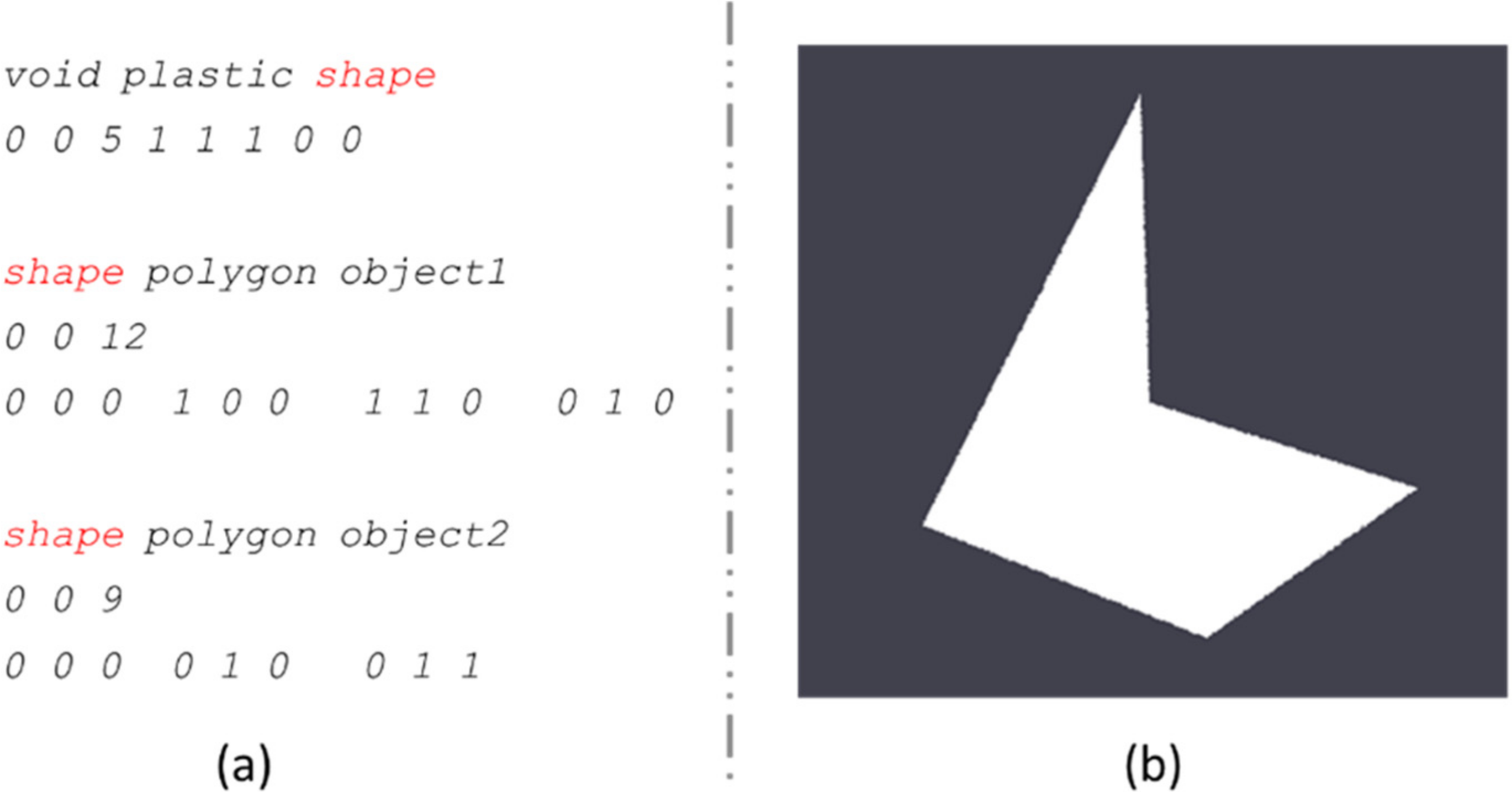
2.3. Specifying Inputs and Interpreting Outputs

As illustrated in Figure 3, the inputs for calculating the view factor between a differential surface and a finite surface with RADIANCE are “differentialSurface”, “surfaceIdentifier” and “surfaceGeometry”. “SurfaceIdentifier” and “surfaceGeometry” relate to the material properties and shape of the finite surface respectively.
Multiple differential surfaces and finite surfaces can be specified at a time by listing them in text files and specifying the path of the text files as the inputs in place of the “surfaceIdentifier” and “differentialSurface”. The results thus generated are a matrix comprising of view factors between individual differential surfaces and finite surfaces.
The format for specifying materials and shapes in RADIANCE is shown in Figure 6. The fundamental material and shape-type that are used for the view factor calculations in this paper are plastic and polygon respectively. Figure 6a describes the general template that can be used for defining plastic and polygon and Figure 6b,c provide an example of each of them, respectively. While RADIANCE supports a multitude of materials and shapes, for the purposes of calculating view factors, the plastic material and the polygon shape are ideal as they can be combined to create complex shapes [29].
Plastic is as an opaque surface that is analogous to conventional diffusing materials assumed in the calculation of view factors. The definition for plastic material as shown in Figure 6b is “void plastic shape 0 0 5 1 1 1 0 0”.
The term “void” indicates that this material is not modified or affected by any other textures or materials. The term “shape” was arbitrarily chosen and can be any combination of ASCII characters. The numbers “0 0 5 1 1 1 0 0” as a whole specify that the reflectance of this material is uniformly diffused white. The three numbers “1 1 1” after “0 0 5” relate to the spectral power of the three channels that RADIANCE employs to describe the color of a surface or a radiation source. These three channels, namely Red, Green, and Blue, relate to primary colors within the human visual system [23].
The definition for a polygon is specified in Figure 6c as “shape polygon object 0 0 12 0 0 …”. Here, the term “shape” indicates that this polygon is of the plastic material type defined in Figure 6b. The term “object” was arbitrarily chosen and can again be any combination of ASCII characters. The numbers “0 0 0 1 0 0 1 1 0 0 1 0” specify the four cartesian coordinates to define the surface shown in Figure 6d. The raytracing methodology implemented in rcontrib, and other RADIANCE programs, has a physical basis. So, finite surfaces are defined according to their actual dimensions. For example, based on the vertices defined in Figure 6c, the resultant polygon shape is a square of unit dimensions. Radiance supports SI units of measurement for distances and the values can be expressed in integer or floating-point numerical format. The units themselves are not specified explicitly in Radiance input formats.
It is possible to combine multiple polygons and materials together. The definition and visualization for a surface comprised of two polygons is shown in Figure 7. Surfaces and surface-combinations of further complexity are visualized in Figure 8.
The methodology to be followed for creating polygons of any number sides is described in detail in [23]. The standard approach for creating complex surfaces for RADIANCE simulations is to model the shape initially in a 3D-Modeling software like AutoCAD®, Sketchup®, Rhino3D® or other similar tools and then export it into a compatible format consisting of polygons. Several free translators and plugins exist for exporting 3D-geometry from CAD software like AutoCAD [30], Sketchup [31] and Rhino3D [32] into RADIANCE format.
As explained previously in Figure 3, differential surfaces are defined as per the format “x y z vx vy vz”. It is possible to specify multiple differential surfaces in a single calculation by listing them in line-separated format. A few examples of multiple differential surfaces are illustrated in Figure 9. Differential surfaces do not have a physical shape or structure in RADIANCE and are intended to specify the location from which rays are to be traced. The cone shapes shown in Figure 9 are intended solely as a means of visualizing their location and orientation. The apex of the cone shapes shown in Figure 9 point in the direction of the vector defined through “vx vy vz”.
As explained in Figure 5, the inputs comprising of finite and differential surfaces need to be sequentially passed to two RADIANCE programs, namely oconv and rcontrib, to generate view factors. A typical calculation process, as executed through the command-line, is shown in Figure 10. The figure shows a simple two-step calculation where the view factor F d A 1 A 2 involving a differential surface dA1 and a finite planar surface A2 is being calculated. The first step involves the creation of the octree from the surface geometry using oconv. The second step invokes rcontrib to calculate the “contribution coefficient” through Monte Carlo raytracing. The octree “geo.oct”, generated through oconv in the previous step, is one of the inputs for rcontrib.
The result from the calculation, a set of three identical numbers, is shown below the rcontrib command in Figure 10. In this example, the contents of the files “sen.rad” and “pts.txt” represent a finite planar surface and differential surface respectively. The contents of both the files are shown in text boxes. The material for the surface i.e., “rectangle”, is specified as the “surfaceIndentifier” using the -m option for rcontrib. The value of ambient bounces (-ab) is not specified as it is set by default to 1 by rcontrib. As described earlier, the numbers relate to the red, green, and blue channels. For the purposes of view factor calculations with uniformly diffused plastic materials (as explained in Section 2.3), the result for each channel will be identical to the other.
As illustrated in the figure, the view factor is obtained by dividing the result from any one of the channels by π. The existence of three channels in the calculation is a feature that is inherent to RADIANCE and cannot be disabled.
For more complex calculations involving multiple differential surfaces, the results can be redirected to an output file. In the next section, we present the validation of the view factor results generated through RADIANCE by considering four simple examples.

3. Validation of RADIANCE Generated Results against Analytical Solutions

The four examples presented in this section are intended to demonstrate the feasibility of calculating view factors between differential surfaces and arbitrary finite planar surfaces with RADIANCE.
Although, as detailed in Section 2.1, RADIANCE has been extensively validated in the last three decades, the validation studies have exclusively focused on lighting and daylighting simulations. Such studies have involved the comparison of empirically measured values of illuminance or luminance with those generated through RADIANCE simulations. To the best of the authors’ knowledge, the results and methodology presented in this paper are the original validation of RADIANCE for the purposes of view factor calculations.
The first two examples involve finite planar surfaces that are perpendicular or parallel to the differential surface. The third example consists of a sphere that is constructed from planar surfaces. The fourth example involves a box whose constituent surfaces surround the differential surface from all sides. In addition to validating the results generated through RADIANCE, the examples presented in this section also constitute the basic steps that are required for calculation of more complex scenarios.

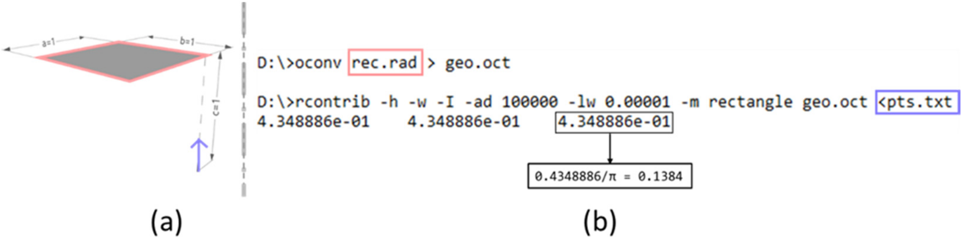
3.1. Differential Element to Finite Parallel Rectangle

The view factor calculation between a differential element and a finite parallel rectangle is shown in Figure 11. As indicated by the figure, the edge lengths a and b of the rectangle are both equal to unity. The distance c of the differential element from the rectangle is one. Additionally, the normal to the differential element passes through a corner of the rectangle. In Figure 11b, the command line parameters -h and -w are intended to turn off information headers and warnings respectively. The parameter -I sets rcontrib in “Irradiance” mode, a setting that is a pre-requisite to calculating view factors.
The analytical solution for this scenario is well-known [33] and can also be accessed through an online interface [34]. The solution can be expressed through Equation (6) as:
F d A 1 A 2 = 1 2 π A 1 + A 2 tan 1 B 1 + A 2 + B 1 + B 2 tan 1 A 1 + B 2
where A = a/c and B = b/c. For a = 1 = b = c, the analytical solution calculated through Equation (6) is 0.1385 when rounded off to four decimal places. The value calculated through RADIANCE, as shown in Figure 11b, is 0.1384. The percentage error calculated as per Equation (7) is 0.072%.
Error = Absolute Analytical   Solution     Radiance   Result Analytical   Solution × 100

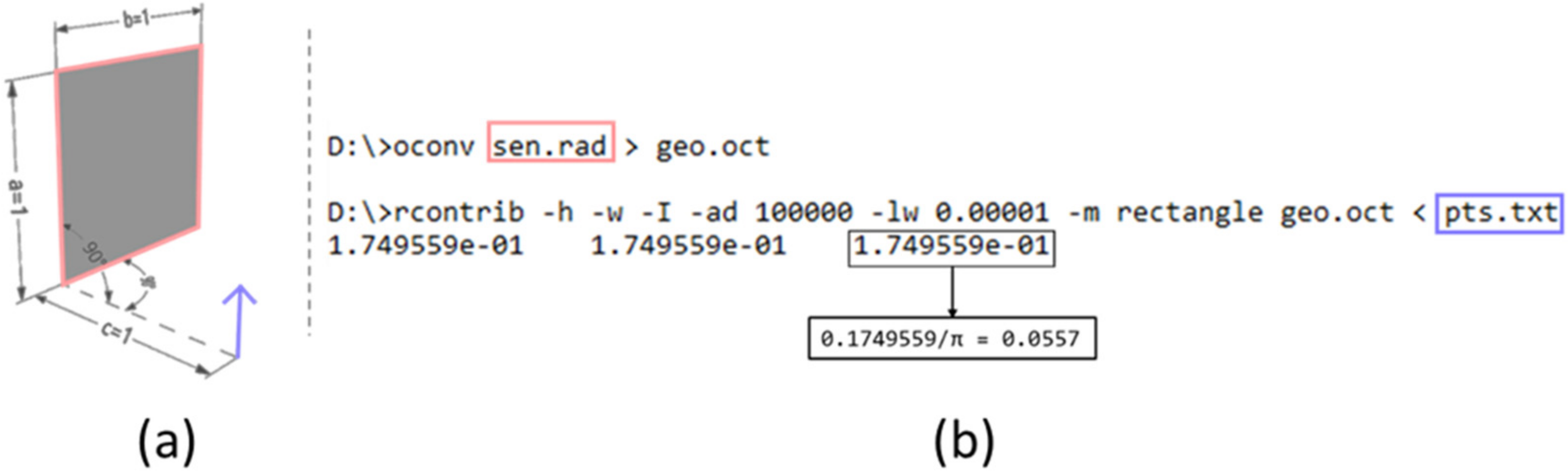
3.2. Differential Element to Rectangle in a Plane at 90° to Plane of Element

Figure 12 shows the view factor calculation for a differential element and a rectangle. The rectangle is in a plane that is oriented at 90° to the plane of the element.
The analytical expression for F d A 1 A 2 in this scenario, provided in [33] and adapted from [34], is:
F d A 1 A 2 = 1 2 π tan 1 1 C C Y tan 1 1 Y
where A = a / b ; C = c / b ; Y = A 2 + B 2 2 . For values of a = 1, b = 1, c = 1 as per the dimensions in Figure 12a, the analytical result rounded off to four decimal places is 0.0557. As shown in Figure 12b this is equal to the result calculated through RADIANCE.

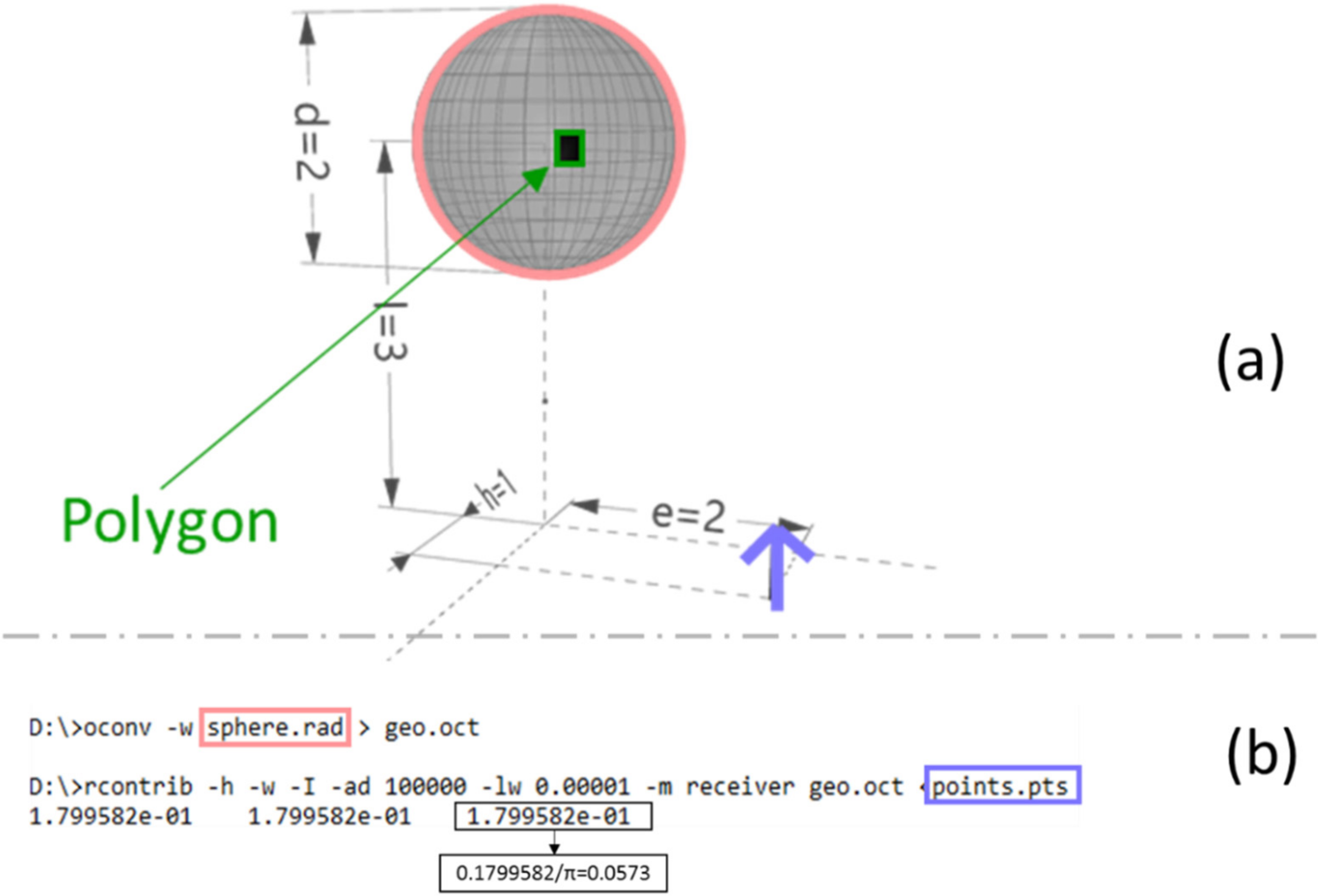
3.3. Element in a Plane to a Sphere

Figure 13 shows the view factor calculation between a differential planar element to a sphere. As highlighted by the single dark polygon on the surface of the sphere in Figure 13a, the spherical surface was approximated by several individual polygons. The view factor can be calculated in such a scenario by using the superposition rule [1]. Assuming a surface J to be composed of N sub-surfaces J1, J2, J3, …, JN, this rule can be mathematically expressed as:
F i J = F i J 1 + F i J 2 + F i J 3 + . + F i J N
For the example considered in Figure 13, the spherical surface was approximated as a composite surface made up of N = 595 planar polygons. The view factor between the differential planar surface and the approximated sphere is then calculated using Equation (9).
An analytical solution for the view factor between a differential element and a sphere was proposed by Naraghi [35]. The analytical solution, adapted from Howell [4], can be expressed as:
F d A 1 A 2 = R 2 1 + E 2 + H 2 3 / 2  
where r = d/2; R = r/l; H = h/l; E = e/l. For the values (d = 2, e = 2, h = 1, l = 3) considered in Figure 13, the analytical solution as per Equation (10), is 0.0573 when rounded off to four decimal places. This is equal to the solution derived through RADIANCE in Figure 13b.

3.4. Energy Balance

Figure 14a shows a differential element that lies at the base of a box and is enclosed by all the remaining sides of the box. The box is defined as a unit cube.
Based on the principle of energy conservation, and the corresponding summation rule for view factors, the sum of view factors from the differential surface to other surfaces should be unity [1]. This can be expressed as general relation through Equation (11) and adapted specifically to Figure 14a through Equation (12). As shown though Figure 14b the result of the view factor calculated with RADIANCE is also 1.
j F d 1 j = 1
F d 1 1 + F d 1 2 + F d 1 3 + F d 1 4 + F d 1 5 + F d 1 6 = 1  
The four examples that were considered for validation in this section featured the same set of raytracing parameters for rcontrib. The relevance of these raytracing parameters, i.e., “-h -w -I -ad 100,000 -lw 0.00001” on the calculation results is discussed later in Section 5. The following section provides a high-level description of how RADIANCE can be used to calculate view factors for scenarios involving complex surfaces and obstructions.

4. View Factors for Complex Shapes and Obstructions

Accommodation of complex geometry and obstructions is a critical aspect of view factor calculations involving urban geometry. For example, view factor calculations between solar panels and the sky vault require the consideration of occluding obstructions like buildings and other urban shapes. The following sub-sections provide a high-level description of how curved shapes and obstructions can be incorporated into calculations.

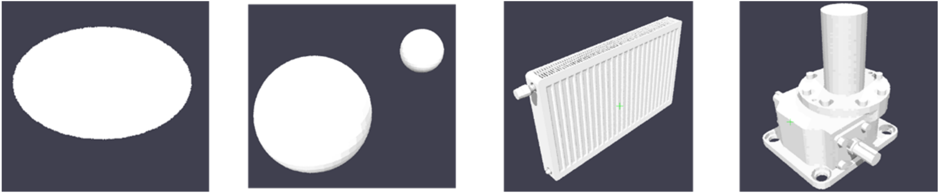
4.1. Complex Shapes with Curvature

While RADIANCE natively supports curved surfaces such as spheres and cones, it does not have the functionality to support other analytical curved shapes. Furthermore, the functionality of exporting complex curved shapes in the form of native RADIANCE spheres or cones is not supported by most 3D modeling software. Consequently, curved shapes must be approximated through planar surfaces.
As shown through the examples in Figure 15, it is possible to generate and thereby calculate view factors shapes of greater complexity by using planar surfaces. The calculation process for these shapes is the same as that discussed for the previous use-cases.

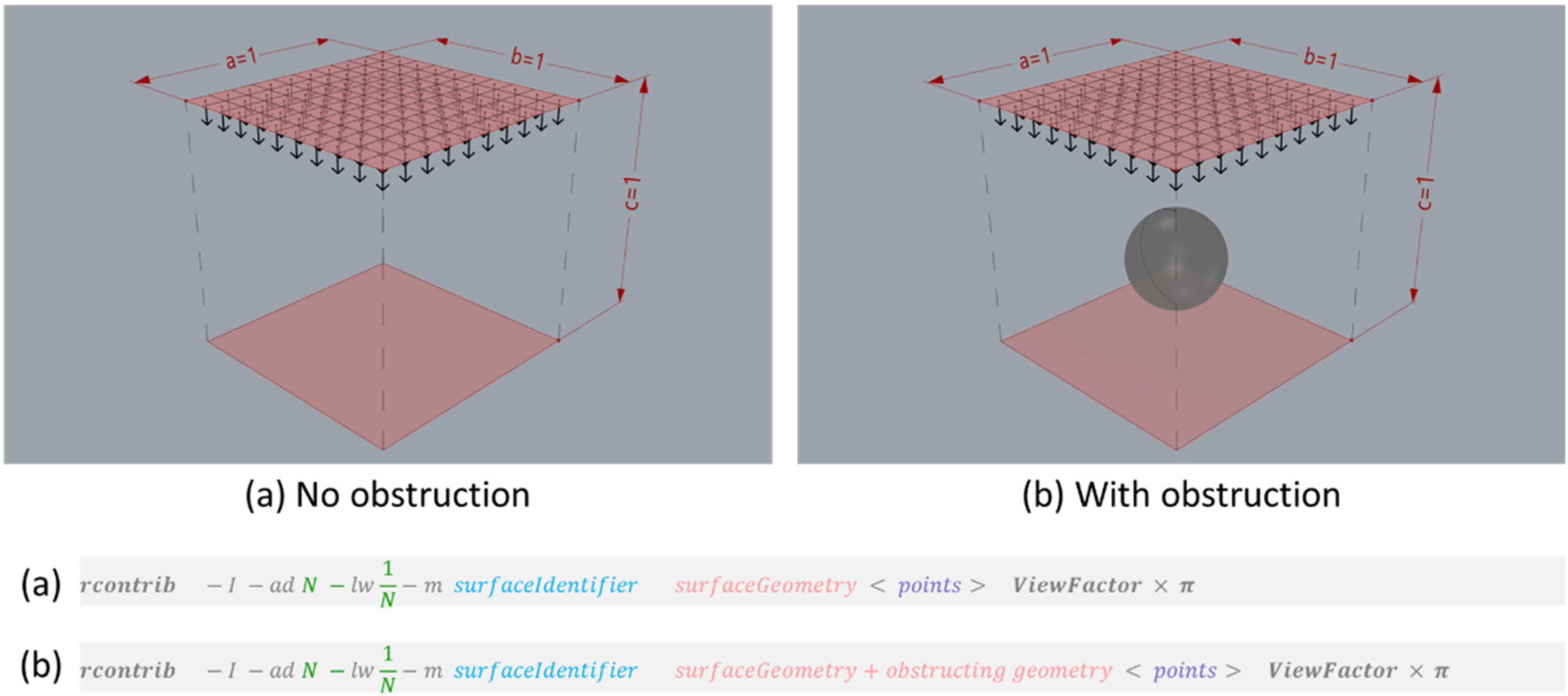
4.2. Incorporating Obstructions

Unlike radiosity-based methods, where including obstructions in view factor calculations necessitates the use of additional algorithms [7], such geometry can be included in a straightforward manner in Radiance [28]. As shown through the equations in Figure 16, incorporating geometry in the calculation only requires adding the surfaces into the contextual geometry. By pre-identifying surfaces whose view factors are being calculated through ray-origins and surfaceIdentifier inputs, the remaining geometry automatically behaves as obstruction.

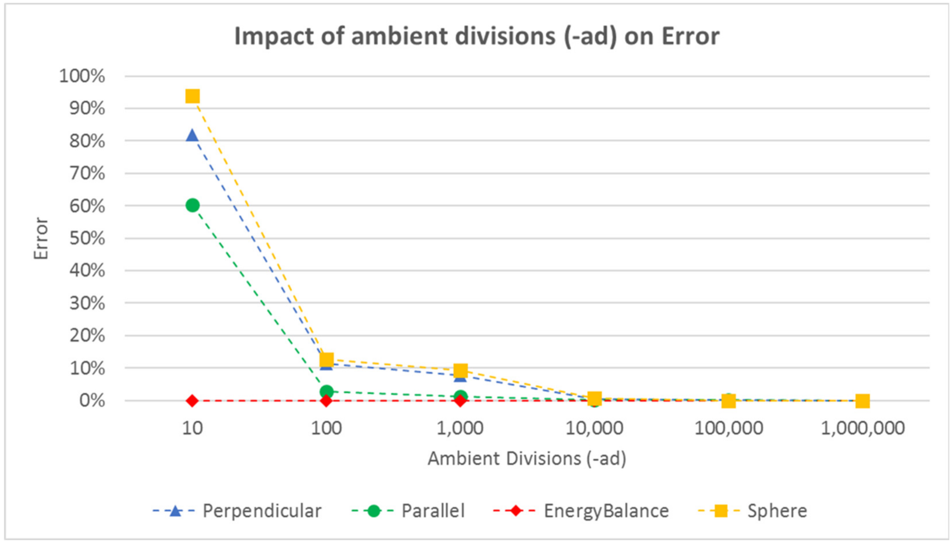
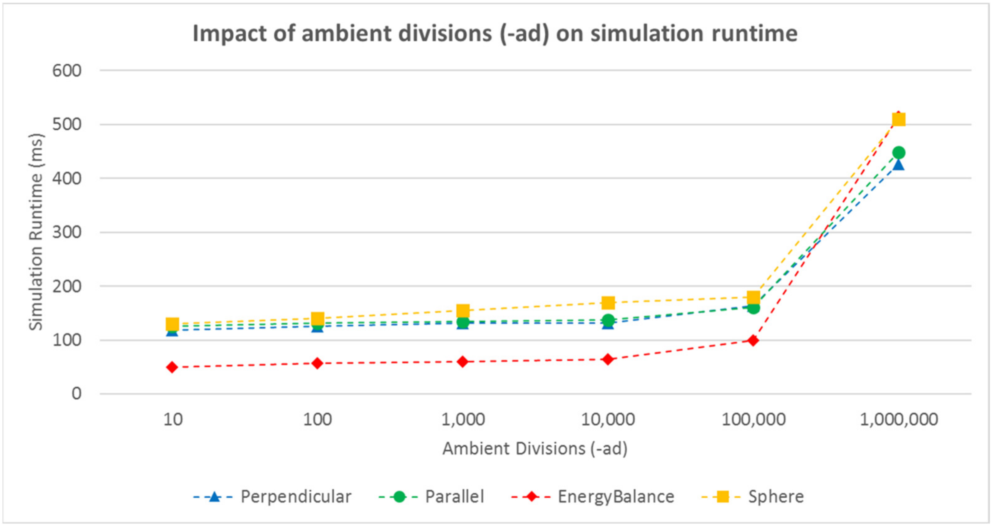
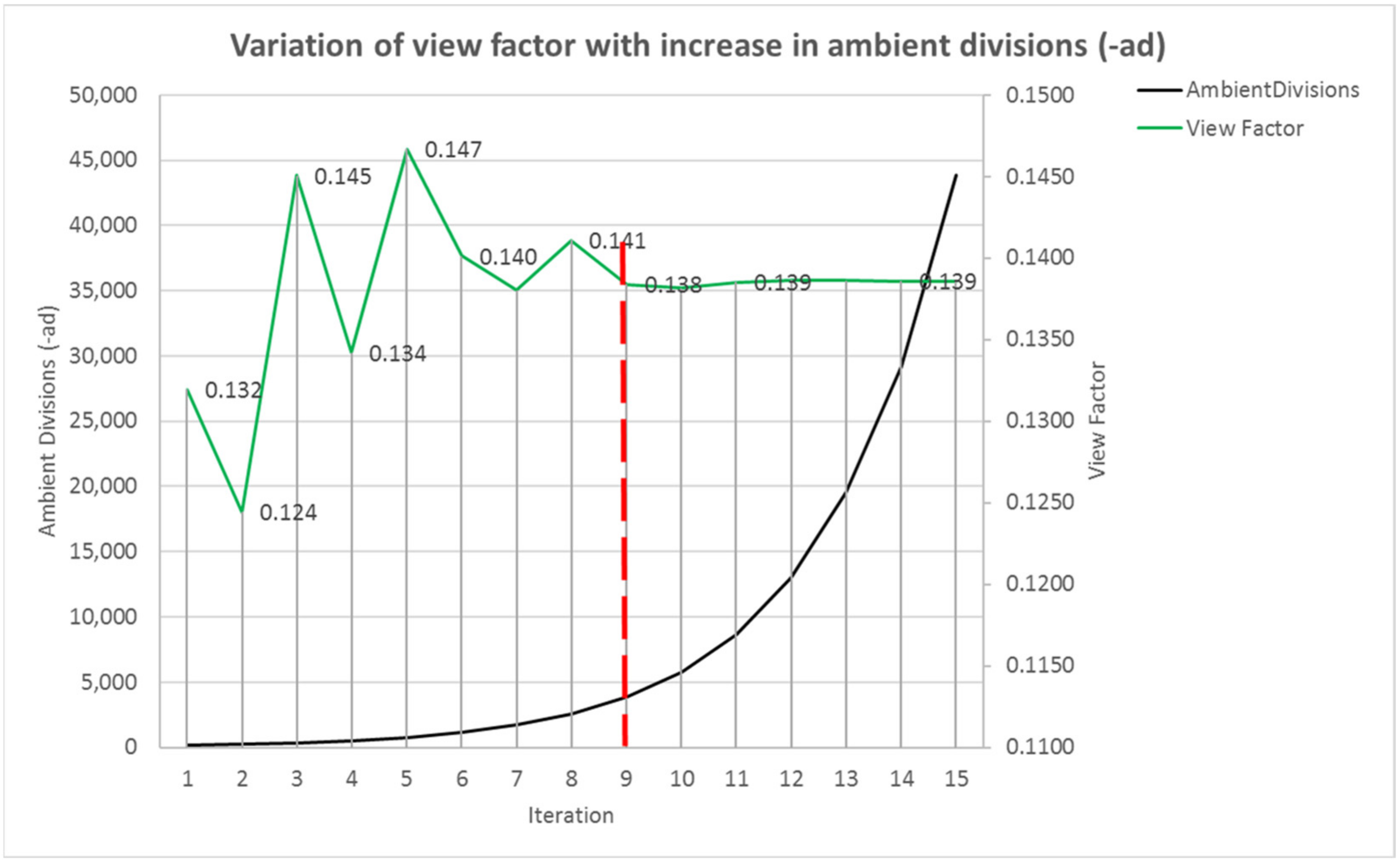
5. Impact of Calculation Parameters on Accuracy, Repeatability of Results, and Runtime

As is true for any probabilistic process that relies on random sampling, increasing the number of samples will yield results that converge. This is demonstrated through Figure 17 where five successive calculations with two values of ambient divisions are shown. The finite and differential surface for the calculation is the same as that for the example discussed in Section 3.1 and Figure 11. The analytical value of the view factor calculated for this calculation is 0.13853. For all other parameters being the same, the results shown in Figure 17a,b compare the impact of ambient divisions, and by extension limit-weight, on the results.
It is evident that for a higher value of ambient divisions (-ad), and correspondingly lower value of limit weight (-lw), the error is consistently lower across successive calculations. Figure 18 provides a broader perspective on the impact of sampling on the results by comparing the error values for the four examples presented in Section 3.1, Section 3.2, Section 3.3 and Section 3.4. The examples are referred to as “Parallel”, “Perpendicular”, “Sphere” and “EnergyBalance” respectively in the plot.
For the values of ambient divisions considered, each calculation was run ten times to calculate an average value of view factor. The rationale for running the calculation multiple times and then averaging results was to minimize the impact of stochastic sampling on the interpretation of results. The average error was calculated as per Equation (7) by considering the result nearest to four decimal places. The error in the case of “EnergyBalance” is 0% for every iteration in that scenario as the random rays originating from the differential surface element were intercepted by the enclosing box irrespective of the magnitude of ambient divisions.
Figure 19 shows the impact of ambient divisions on the average calculation runtime. All the calculations were run on a dedicated Intel i5-8400 2.80 GHz computer with six cores and 16GB of RAM. While the exact runtimes are specific to the machine, the trends shown provide a general indication that the calculation runtime increases with an increase in ambient divisions. The non-linear trend in the plot after 100,000 ambient divisions is attributable to the processing limit of the computer being reached.
The plots in Figure 18 and Figure 19 convey that there is a trade-off between the calculation runtime and accuracy. The accuracy of the calculation can be improved by increasing sampling through ambient divisions. As indicated by the error values for 10,000 divisions and above in Figure 17, beyond a certain extent, the improvements in accuracy might not be discernible.

6. Discussion

All the examples considered in this paper have analytical solutions and were chosen for that specific reason. As demonstrated in Section 5, setting a high value for ambient divisions will ensure that the result obtained is within desired tolerance limits (of say 0.5%). However, knowing whether the result is within tolerance is predicated on knowing the result of the calculation upfront.
In non-standard cases where no analytical expressions exist and RADIANCE is being used to calculate the view factor, a convergence criterion can be defined by progressively increasing the ambient parameters between successive calculations. The result from every calculation can be compared with the results from the previous calculations to determine the variability in results. An example of this is shown through a chart in Figure 20, which compares the variation in view factor as a function of ambient divisions.
The ambient divisions (black line) and calculated view factor (green line) shown here relate to the scenario presented in Section 3.1, i.e., view factor between differential planar element to finite parallel rectangle. The ambient division for the first iteration was set to 100 and increased by 50% for every subsequent iteration. So, for example, the second, third and final iterations had 150, 225, and 43,790 (rounded to nearest integer) ambient divisions, respectively. As highlighted by the red dotted line, the results stabilize beyond the ninth calculation where the ambient divisions are less than 5000.

7. Conclusions

The primary aim of this research was to demonstrate the methodology of employing RADIANCE as a view factor calculation tool. As illustrated through the several examples for finite and differential surfaces in Section 3, RADIANCE can be effectively used to calculate view factors for a variety of surfaces through the standard Monte Carlo method. View factors can be calculated with only a couple of the over 100 programs that are present in the RADIANCE suite. So, the steep learning curve that has traditionally been associated with using RADIANCE for lighting calculations is not applicable to the calculation of view factors.
As discussed previously, a majority—if not all—of the view factor calculation tools developed in the past few decades are currently not under active development. Consequently, the functionalities of these tools have not been updated to leverage the advancements in computing hardware and operating systems. In contrast, RADIANCE is still being actively developed and maintained by its core developer as well as the principal funding agency. This is attributable partly to its relatively large user base and prominence as an industry- and research-grade simulation tool. RADIANCE can be used on multiple operating systems and computing platforms such as commercial cloud-based computing systems.
The primary advantage for RADIANCE, when compared to existing view factor calculation tools, lies in its ability to efficiently handle complex geometries that are likely to be found in building simulations in both indoor and outdoor contexts. Conventional radiosity-based tools typically support only planar shapes and require extensive calculation time. As shown by the examples in Section 3, irrespective of the shape and size of a surface, RADIANCE provides a singular approach for calculating view factors. Furthermore, the availability of free plugins and translation tools to export geometry from common building 3D modeling software to RADIANCE makes it possible to generate, and calculate, view factors for virtually any scale and form of surfaces.
The calculation methodology proposed in this research can be applied to tools such as EnergyPlus and ESP-r to incorporate complex, non-planar shapes into building energy simulations. Currently such tools rely on approximating complex building geometry generated through 3D modeling software such as Revit and Rhino3D into simple planar surfaces. Several studies have already documented the coupling or co-simulation of RADIANCE with building energy simulation tools for performing more physically accurate lighting simulations with complex geometries. Similarly, in such workflows the calculation of view factors too can be performed through RADIANCE by either using the same model from lighting simulations or exporting a dedicated model through one of the freely available open-source translators.
The authors intend to disseminate the automation scripts for calculating view factors through 3D modeling software on open-source platforms. Future research will address the application of this tool to simultaneously calculate view factors of multiple surfaces and validate the examples with obstructions by comparing them with analytically derived solutions.

Author Contributions

Conceptualization, S.S.; methodology and software, S.S. and G.W.; formal analysis and validation, S.S. and S.T.; writing—original draft preparation, S.S and S.H.; writing—review and editing, S.S., S.H., S.T. and G.W.; supervision, S.H., S.T. and G.W. All authors have read and agreed to the published version of the manuscript.

Funding

This research received no external funding.

Institutional Review Board Statement

Not applicable.

Informed Consent Statement

Not applicable.

Conflicts of Interest

The authors declare that they have no potential conflict of interest regarding this research work.

Nomenclature

A 1 ,   A 2 Two arbitrarily oriented surfaces
d A 1 ,   d A 2 
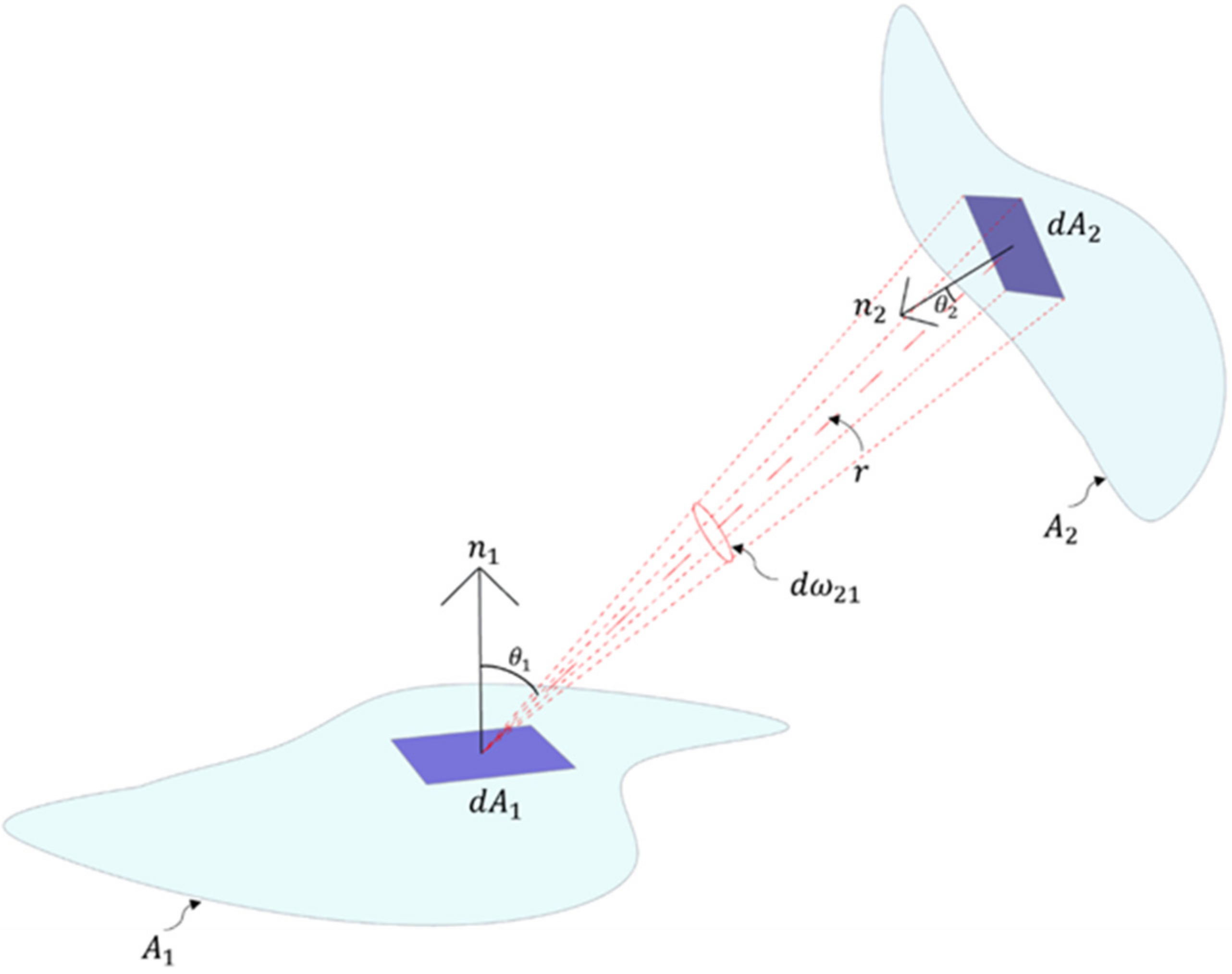
Differential surface elements of A1 and A2 respectively.
F12Diffuse view factor from surface A1 to A2.
F d A 1 d A 2 Diffuse view factor from surface dA1 to dA2.
θ 1 The angle between the surface-normal of dA1 and the line connecting dA1 and dA2
θ 2 The angle between the surface-normal of dA2 and the line connecting dA1 and dA2
r Distance between surfaces dA1 and dA2
θPolar angle measured from the surface normal.
φAzimuthal angle.
L r θ r , φ r Reflected radiance in W/(sr*m2),
L e θ r , φ r Emitted radiance in W/(sr*m2)
L i θ i , φ i ρ b d Incident radiance in W/(sr*m2),
ρ b d θ i , φ i ; θ r , φ r Bidirectional reflectance-transmittance distribution function in sr−1
E i n d θ i , φ i Indirect irradiance in W/m2
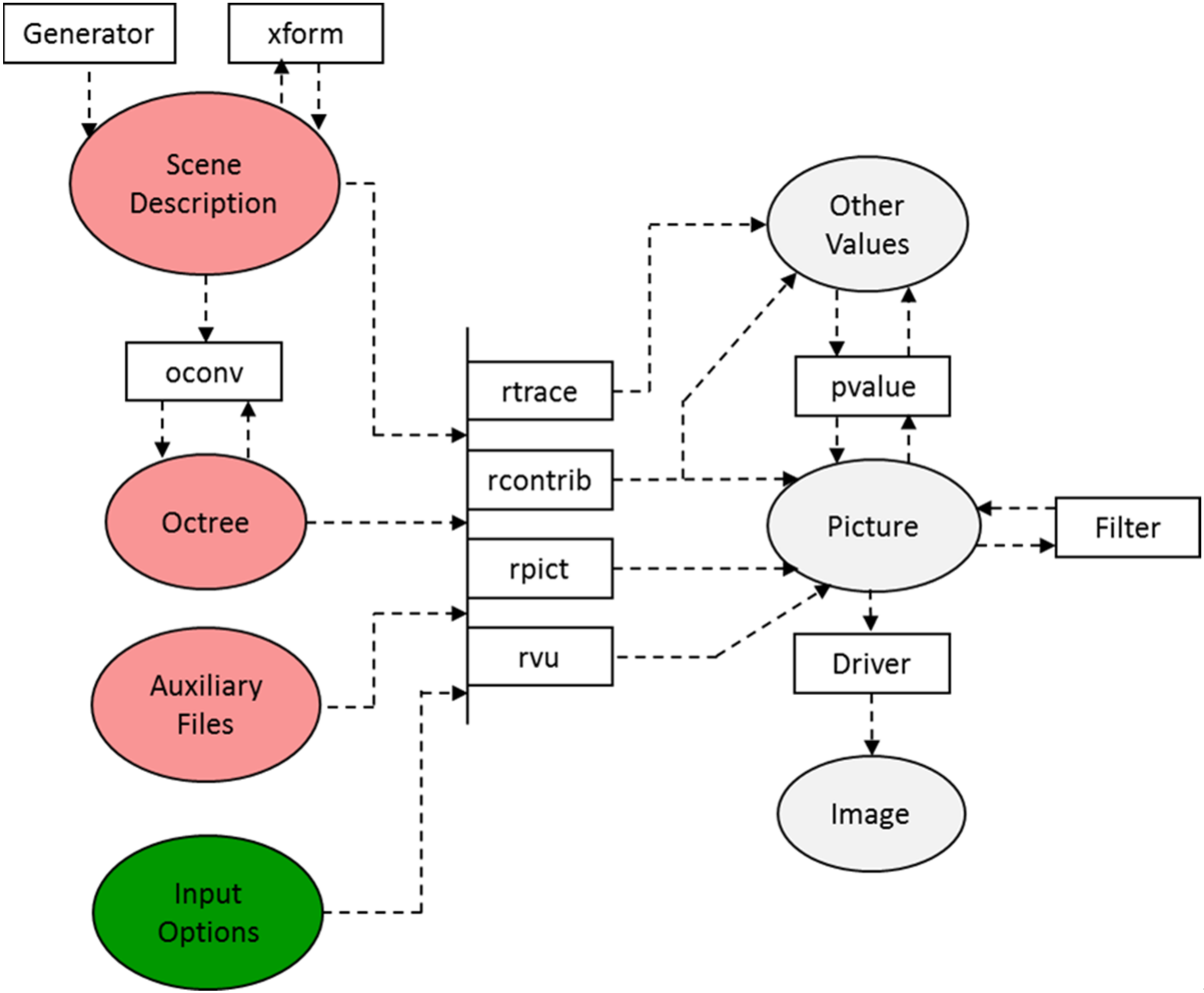
oconvRADIANCE program that is used for creating an octree structure.
rcontribRADIANCE program that is used for raytracing.
-Ircontrib option that assigns irradiance mode of calculation.
-adrcontrib option that specifies the number of ambient divisions.
-abrcontrib option that specifies the number of ambient bounces.
-lwrcontrib option to specify the limit weight parameter.
-mrcontrib option to specify the modifier of the finite surface whose view factor is to be calculated.
-wrcontrib option to turn off warnings.
-hrcontrib option to turn off the header. This enables only the result of the calculation being generated as the output.

References

  1. Cengel, Y. Heat and Mass Transfer: Fundamentals and Applications; McGraw-Hill Higher Education: New York, NY, USA, 2015; ISBN 9780072458930. [Google Scholar]
  2. Hensen, J.L.M.; Lamberts, R. Building Performance Simulation for Design and Operation, 2nd ed.; Routledge: London, UK, 2019; ISBN 9781138392199. [Google Scholar]
  3. Gupta, M.K.; Bumtariya, K.J.; Shukla, H.; Patel, P.; Khan, Z. Methods for Evaluation of Radiation View Factor: A Review. Mater. Today Proc. 2017, 4, 1236–1243. [Google Scholar] [CrossRef]
  4. Howell, J.R.; Menguc, M.P.; Siegel, R. Thermal Radiation Heat Transfer; CRC Press: Boca Raton, FL, USA, 2010; ISBN 9781439894552. [Google Scholar]
  5. Spencer, S.N. The Hemisphere Radiosity Method: A Tale of Two Algorithms. In Photorealism in Computer Graphics; Bouatouch, K., Bouville, C., Eds.; Springer: Berlin/Heidelberg, Germany, 1992; pp. 127–135. [Google Scholar]
  6. Cohen, M.F.; Greenberg, D.P. The hemi-cube: A radiosity solution for complex environments. ACM SIGGRAPH Comput. Graph. 1985, 19, 31–40. [Google Scholar] [CrossRef]
  7. Walton, G. Calculation of Obstructed View Factors by Adaptive Integration; National Institute of Standards and Technology: Gaithersburg, MD, USA, 2002. [Google Scholar]
  8. Howell, J.R. Application of Monte Carlo to Heat Transfer Problems. Adv. Heat Transfer 1969, 5, 1–54. [Google Scholar] [CrossRef]
  9. Hien, V.D.; Chirarattananon, S. Triangular Subdivision for the Computation of Form Factors. LEUKOS 2005, 2, 41–59. [Google Scholar] [CrossRef]
  10. Vujičić, M.R.; Lavery, N.P.; Brown, S.G.R. View factor calculation using the Monte Carlo method and numerical sensitivity. Commun. Numer. Methods Eng. 2005, 22, 197–203. [Google Scholar] [CrossRef]
  11. Mirhosseini, M.; Saboonchi, A. View factor calculation using the Monte Carlo method for a 3D strip element to circular cylinder. Int. Commun. Heat Mass Transf. 2011, 38, 821–826. [Google Scholar] [CrossRef]
  12. He, F.; Shi, J.; Zhou, L.; Li, W.; Li, X. Monte Carlo calculation of view factors between some complex surfaces: Rectangular plane and parallel cylinder, rectangular plane and torus, especially cold-rolled strip and W-shaped radiant tube in continuous annealing furnace. Int. J. Therm. Sci. 2018, 134, 465–474. [Google Scholar] [CrossRef]
  13. MacFarlane, J. VISRAD—A 3-D view factor code and design tool for high-energy density physics experiments. J. Quant. Spectrosc. Radiat. Transf. 2003, 81, 287–300. [Google Scholar] [CrossRef] [Green Version]
  14. Maltby, J.D.; Zeeb, C.N.; Dolaghan, J.; Burns, P.J. User’s Manual for MONT2D-Version 2.6 and MONT3D-Version 2.3; Colorado State University: Fort Collins, CO, USA, 1994. [Google Scholar]
  15. Ward, G.J.; Rubinstein, F.M.; Clear, R.D. A ray tracing solution for diffuse interreflection. ACM SIGGRAPH Comput. Graph. 1988, 22, 85–92. [Google Scholar] [CrossRef]
  16. Ward, G.J.; Rubinstein, F.M. A New Technique for Computer Simulation of Illuminated Spaces. J. Illum. Eng. Soc. 1988, 17, 80–91. [Google Scholar] [CrossRef]
  17. Ward, G.; Rubinstein, F.; Grynberg, A. Luminance in computer-aided lighting design. In Proceedings of the 1st Building Simulation Conference, Vancouver, BC, Canada, 23–24 June 1989. [Google Scholar]
  18. Ward, G.J.; Heckbert, P.S. Irradiance gradients. In Proceedings of the Third Eurographics Workshop on Rendering, Bristol, UK, 17–20 May 1992. [Google Scholar]
  19. Grynberg, A. Validation of Radiance. LBNL. 1989. Available online: https://eta-publications.lbl.gov/sites/default/files/lbid-1575.pdf (accessed on 20 February 2022).
  20. Mardaljevic, J. Validation of a lighting simulation program under real sky conditions. Light. Res. Technol. 1995, 27, 181–188. [Google Scholar] [CrossRef]
  21. McNeil, A.; Lee, E.S. A validation of the Radiance three-phase simulation method for modelling annual daylight performance of optically complex fenestration systems. J. Build. Perform. Simul. 2013, 6, 24–37. [Google Scholar] [CrossRef]
  22. Lee, E.S.; Geisler-Moroder, D.; Ward, G. Modeling the direct sun component in buildings using matrix algebraic approaches: Methods and validation. Sol. Energy 2018, 160, 380–395. [Google Scholar] [CrossRef] [Green Version]
  23. Ward, G.; Shakespeare, R.; Ehrlich, C.; Mardaljevic, J.; Phillips, E.; Apian-Bennewitz, P. Rendering with Radiance: The Art and Science of Lighting Visualization; Morgan Kaufmann: San Francisco, CA, USA, 1998; ISBN 0974538108. [Google Scholar]
  24. Ward, G.; Mistrick, R.; Lee, E.S.; McNeil, A.; Jonsson, J. Simulating the Daylight Performance of Complex Fenestration Systems Using Bidirectional Scattering Distribution Functions within Radiance. LEUKOS 2011, 7, 241–261. [Google Scholar] [CrossRef] [Green Version]
  25. LBNL. Rcontrib. 2016. Available online: https://www.radiance-online.org/learning/documentation/manual-pages/pdfs/rfluxmtx.pdf (accessed on 20 February 2022).
  26. Shirley, P.; Chiu, K. A Low Distortion Map Between Disk and Square. J. Graph. Tools 1997, 2, 45–52. [Google Scholar] [CrossRef]
  27. Glassner, A.S. Space subdivision for fast ray tracing. IEEE Comput. Graph. Appl. 1984, 4, 15–24. [Google Scholar] [CrossRef]
  28. Ward, G.J. The RADIANCE lighting simulation and rendering system. In Proceedings of the 21st Annual Conference on Computer Graphics and Interactive Techniques—SIGGRAPH ’94, Orlando, FL, USA, 24–29 July 1994; pp. 459–472. [Google Scholar]
  29. Ward, G. Radiance File Formats. 1997. Available online: https://floyd.lbl.gov/radiance/refer/filefmts.pdf (accessed on 20 February 2022).
  30. Konstantinos, M.P. Desktop Radiance: A New Tool for Computer-Aided Daylighting Design. ACADIA Q. 2000, 19, 2. [Google Scholar]
  31. Bleicher, T. su2rad—Radiance Exporter for SketchUp. In Proceedings of the 7th International Radiance Workshop, Fribourg, Switzerland, 30–31 October 2008. Available online: https://www.radiance-online.org:447/radiance-workshop7/Content/Bleicher/su2rad.pdf (accessed on 20 February 2022).
  32. Roudsari, M.; Pak, M. Ladybug: A Parametric Environmental Plugin for Grasshopper to Help Designers Create an Environmentally-Conscious Design. In Proceedings of the 13th Conference of International Building Performance Simulation Association, Chambery, France, 25–28 August 2013. [Google Scholar]
  33. Hamilton, D.C.; Morgan, W. Radiant-Interchange Configuration Factors. NASA. 1952. Available online: https://ntrs.nasa.gov/citations/19930083529 (accessed on 20 February 2022).
  34. Howell, J.R. A Catalog of Radiation Transfer Configuration Factors. 2001. Available online: http://www.thermalradiation.net/indexCat.html (accessed on 20 February 2022).
  35. Naraghi, M.H.N. Radiative View Factors from Spherical Segments to Planar Surfaces. J. Thermophys. Heat Transf. 1988, 2, 373–375. [Google Scholar] [CrossRef]
Figure 1. The geometry and variables for calculating view factor between two surfaces A1 and A2.
Applsci 12 02768 g001
Figure 2. Schematic diagram for a conventional RADIANCE simulation. The values in rectangles refer to individual executable programs. The programs ‘Generator’, ‘Driver’ and ‘Filter’ refer to generic third-party programs that interface with RADIANCE inputs and outputs.
Applsci 12 02768 g002
Figure 3. Calculation of view factor between a differential surface and a finite surface with rcontrib. The dots on the finite surface in (a) indicate the sampling controlled by the -ad parameter. As shown by (b), increased sampling will improve the estimation of the view factor. An explanation of the terms in the syntax (c) is provided in the nomenclature.
Applsci 12 02768 g003
Figure 4. An illustration of the original sampling pattern employed in RADIANCE. The dots represent individual samples over the projected hemisphere [23].
Applsci 12 02768 g004
Figure 5. The proposed workflow for calculating view factors with RADIANCE. RADIANCE programs are identified through rectangles, and inputs and outputs are denoted through ellipses. The dotted figures represent a script and output that is external to RADIANCE. The colors used in this figure are complimentary to the ones used in Figure 3c.
Applsci 12 02768 g005
Figure 6. Specifying materials and shapes in RADIANCE. (a) Shows the general template. (b,c) Provide examples of a material type and shape type respectively. (d) shows a visualization of the geometry defined through the combination of (b,c).
Applsci 12 02768 g006
Figure 7. A surface comprised of two polygons and same material. (a) Shows the definition of the surface in ASCII format and (b) shows a RADIANCE-rendered image of the surface.
Applsci 12 02768 g007
Figure 8. Surfaces created by using multiple polygons. All the surfaces shown above were first modeled in Sketchup® and then exported into the RADIANCE format using the plugin Su2Rad.
Applsci 12 02768 g008
Figure 9. Different configurations of differential surfaces that can be specified through a single file, and therefore can be used in a single calculation. The shape in (a) illustrates a single differential surface. Shapes in (b,c) illustrate differential surfaces aligned along a line and distributed across an area respectively. The shape shown in (d) illustrates surface normals of planar surfaces that were created by subdividing a spherical surface.
Applsci 12 02768 g009
Figure 10. An illustration of the command-line process for calculating view factors with RADIANCE.
Applsci 12 02768 g010
Figure 11. View factor calculation between a differential planar element and finite parallel rectangle. The geometry is shown in (a) and a screen-capture of the corresponding RADIANCE calculation is shown in (b).
Applsci 12 02768 g011
Figure 12. View factor between a differential planar element to rectangle in plane 90° to plane of element as shown in (a) with the corresponding calculation in (b).
Applsci 12 02768 g012
Figure 13. View factor between a differential planar element and a sphere as shown in (a) with the corresponding calculation in (b). The sphere considered for the calculation is comprised of 595 polygons. The sphere in (a) shows a reduced number of polygons to improve legibility of the figure.
Applsci 12 02768 g013
Figure 14. View factor between a differential surface, indicated by the purple arrow in (a), and surfaces of a box that encloses it. The corresponding calculation is shown in (b).
Applsci 12 02768 g014
Figure 15. An assortment of curved shapes whose view factors can be calculated by the planar sub-division and ray-arrangement for each shape. As explained previously, once the view factors between rays and finite planar shapes have been calculated, further results can be derived through superposition rule. (a,c) Show open and closed curved surfaces respectively while (b) shows two open flat surfaces.
Applsci 12 02768 g015
Figure 16. A comparison of the geometric setup and corresponding command-line arguments for view factor calculations without obstruction (a) and with obstruction (b). In (b), the additional sphere constitutes the obstruction.
Applsci 12 02768 g016
Figure 17. The impact of sampling parameters on accuracy and repeatability of results in five successive calculations. (a) Denotes low parameters with values of 100 and 0.01 for -ad and -lw respectively, and (b) denotes high parameters.
Applsci 12 02768 g017
Figure 18. The variation in average error as per ambient divisions for the calculations considered in Section 3.1 (Parallel), Section 3.2 (Perpendicular), Section 3.3 (Sphere) and Section 3.4 (EnergyBalance).
Applsci 12 02768 g018
Figure 19. Variation in average calculation runtime according to ambient divisions.
Applsci 12 02768 g019
Figure 20. Variation of results with progressive increase in sampling controlled through ambient divisions.
Applsci 12 02768 g020
Publisher’s Note: MDPI stays neutral with regard to jurisdictional claims in published maps and institutional affiliations.

