
An Overview on Deep Learning Techniques for Video Compressive Sensing


Abstract
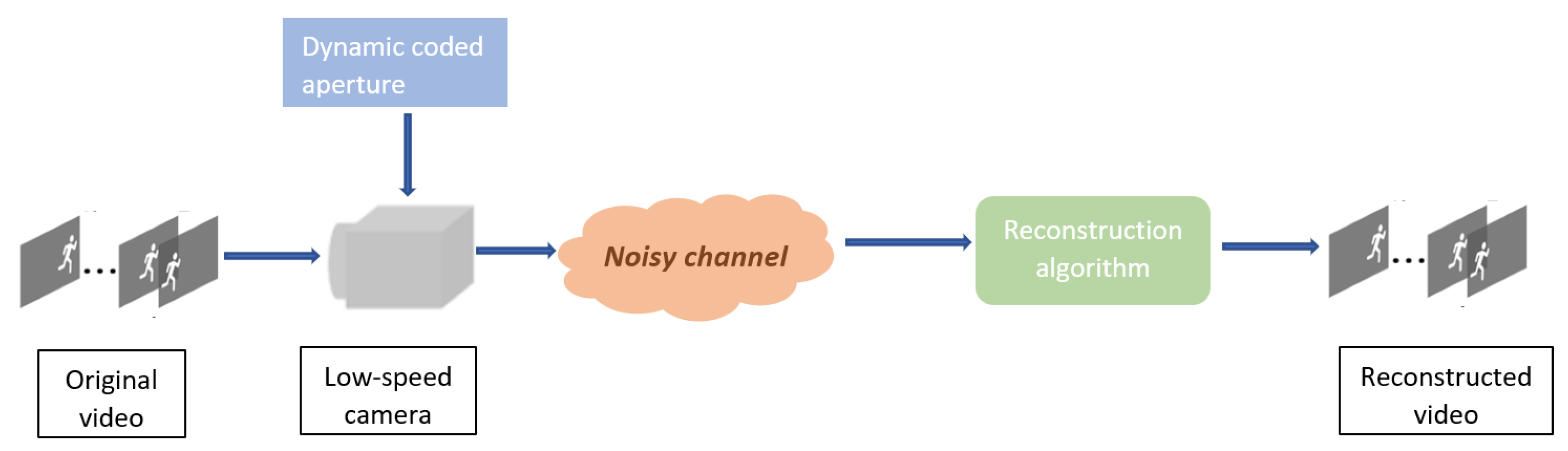
:1. Introduction
2. Compressive Sensing
2.1. Mathematical Introduction
2.2. Sensing Matrix
2.3. Reconstruction Algorithms
2.3.1. Convex Optimization
2.3.2. Greedy Algorithms
3. Image Compressive Sensing
4. Video Compressive Sensing
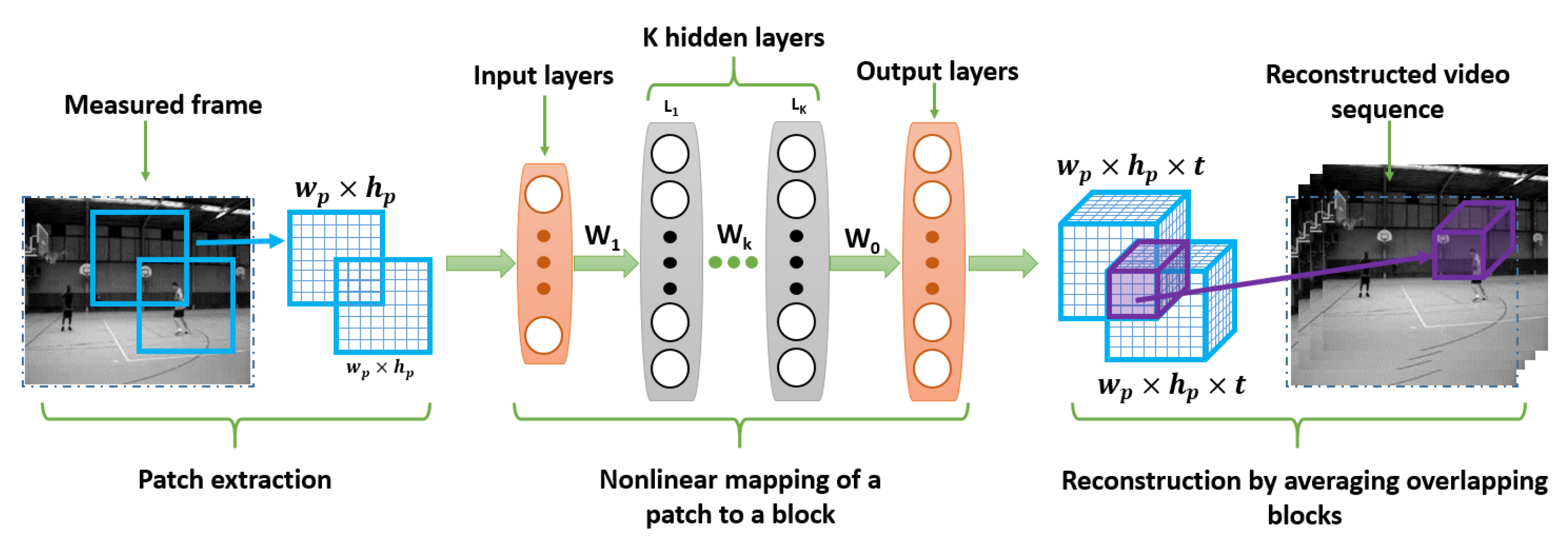
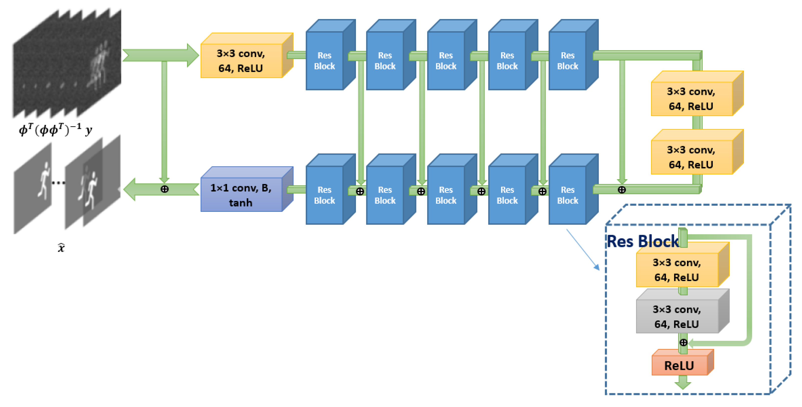
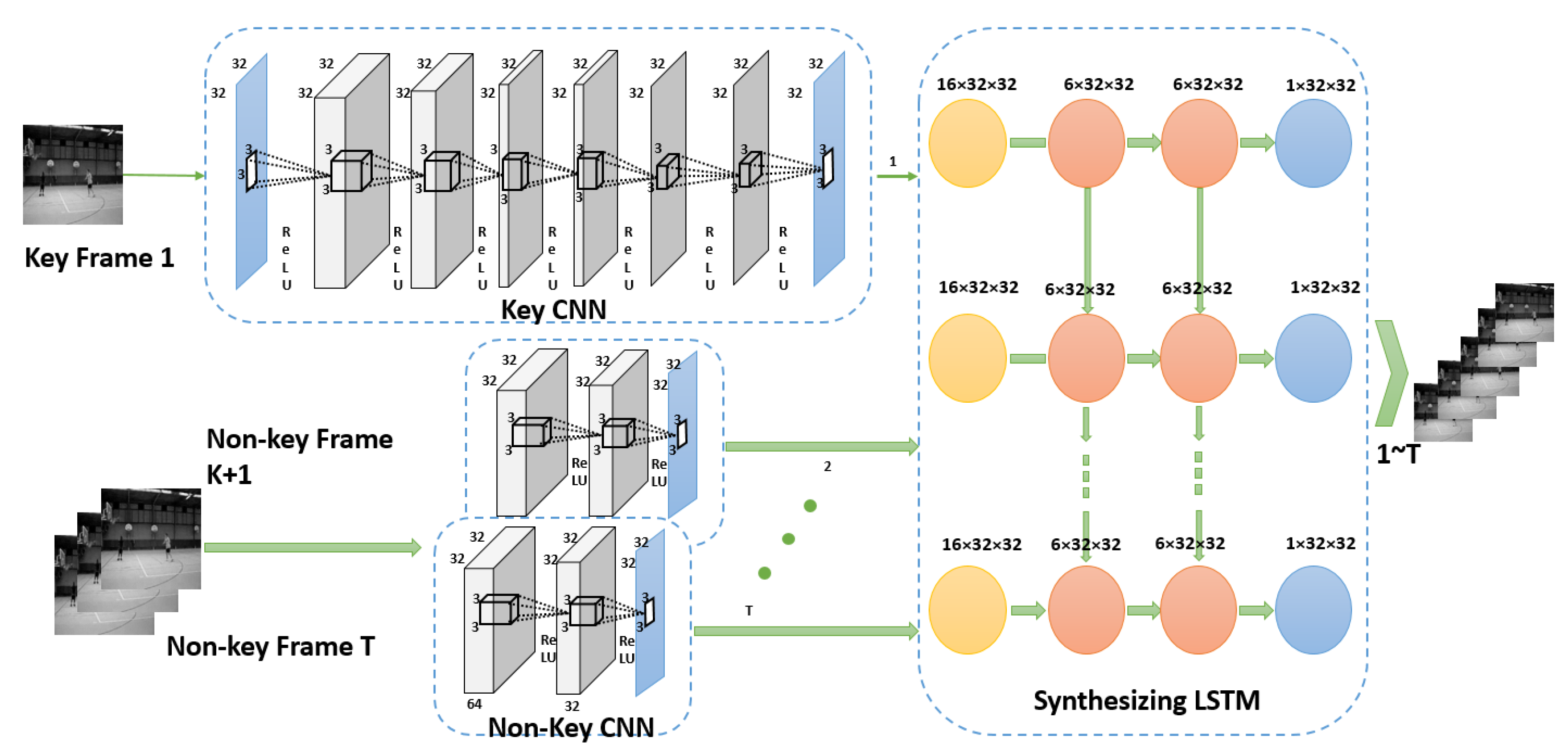
4.1. Temporal VCS
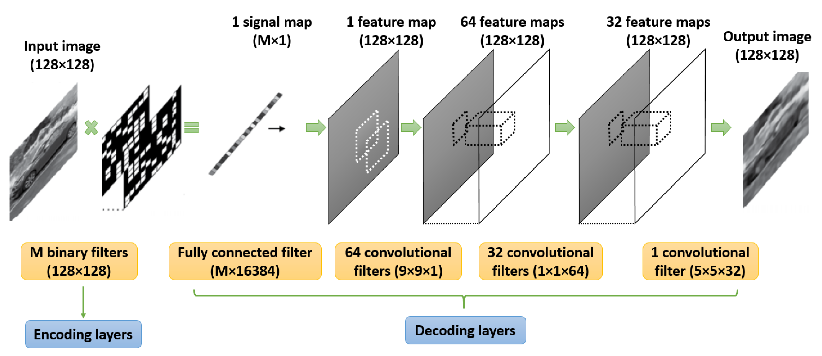
4.2. Spatial VCS
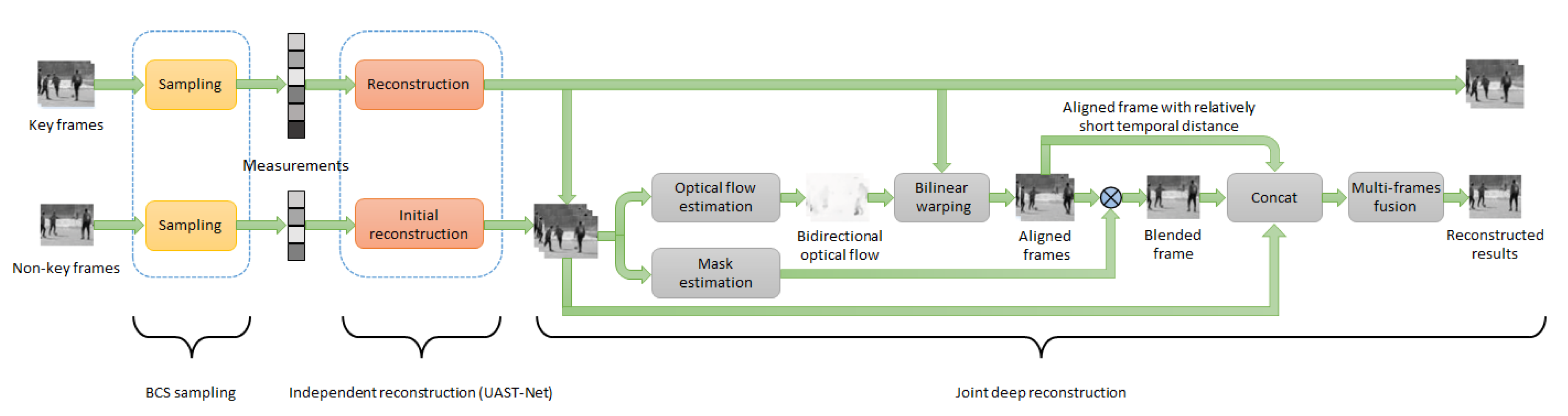
4.3. Spatio-Temporal VCS
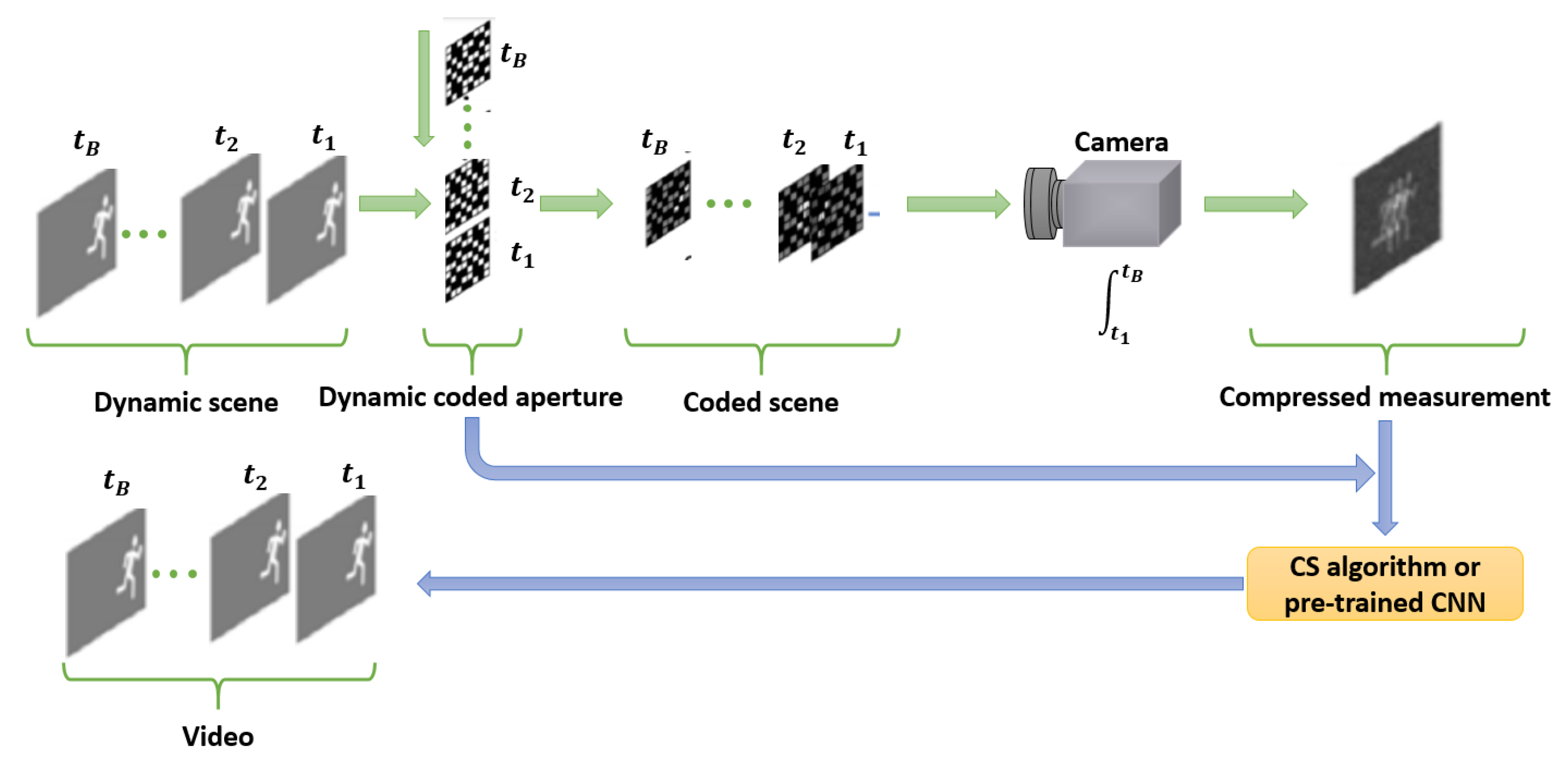
5. Video Single-Pixel Imaging and Video Snapshot Compressive Imaging
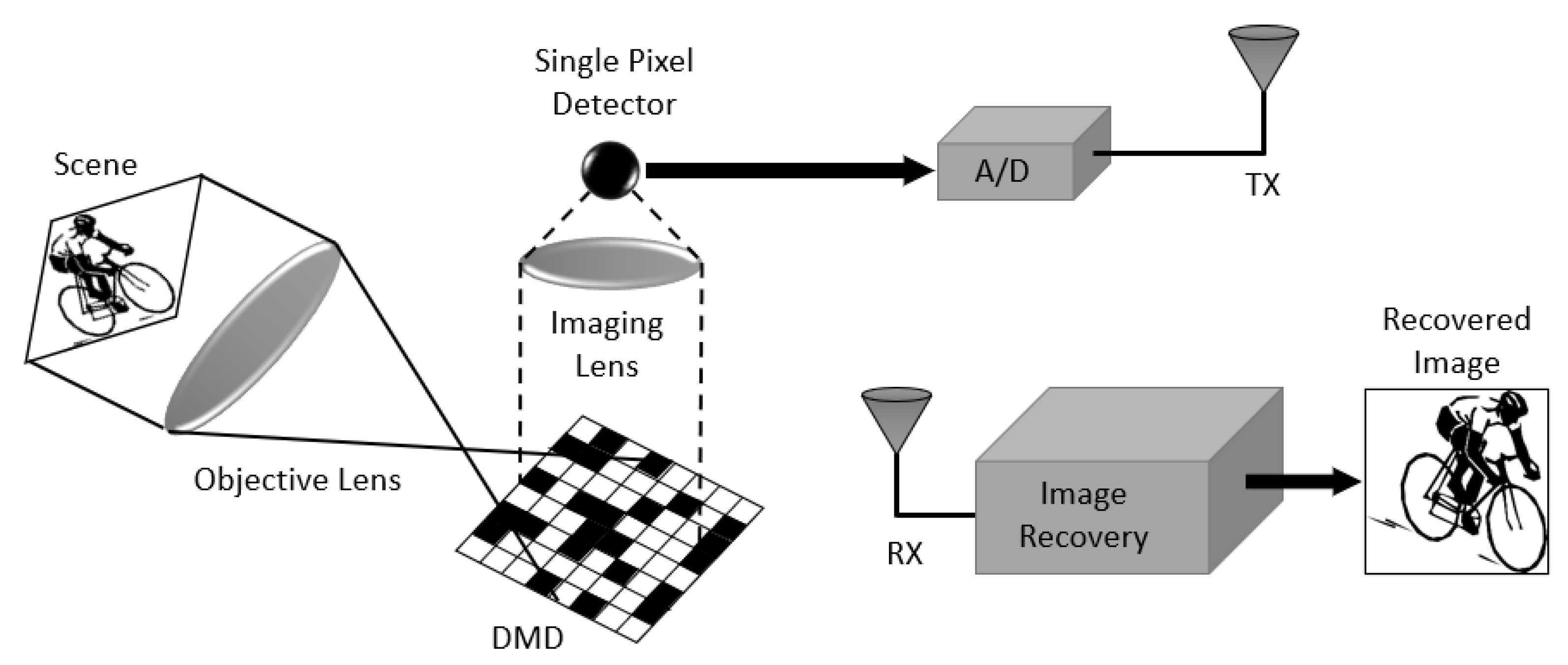
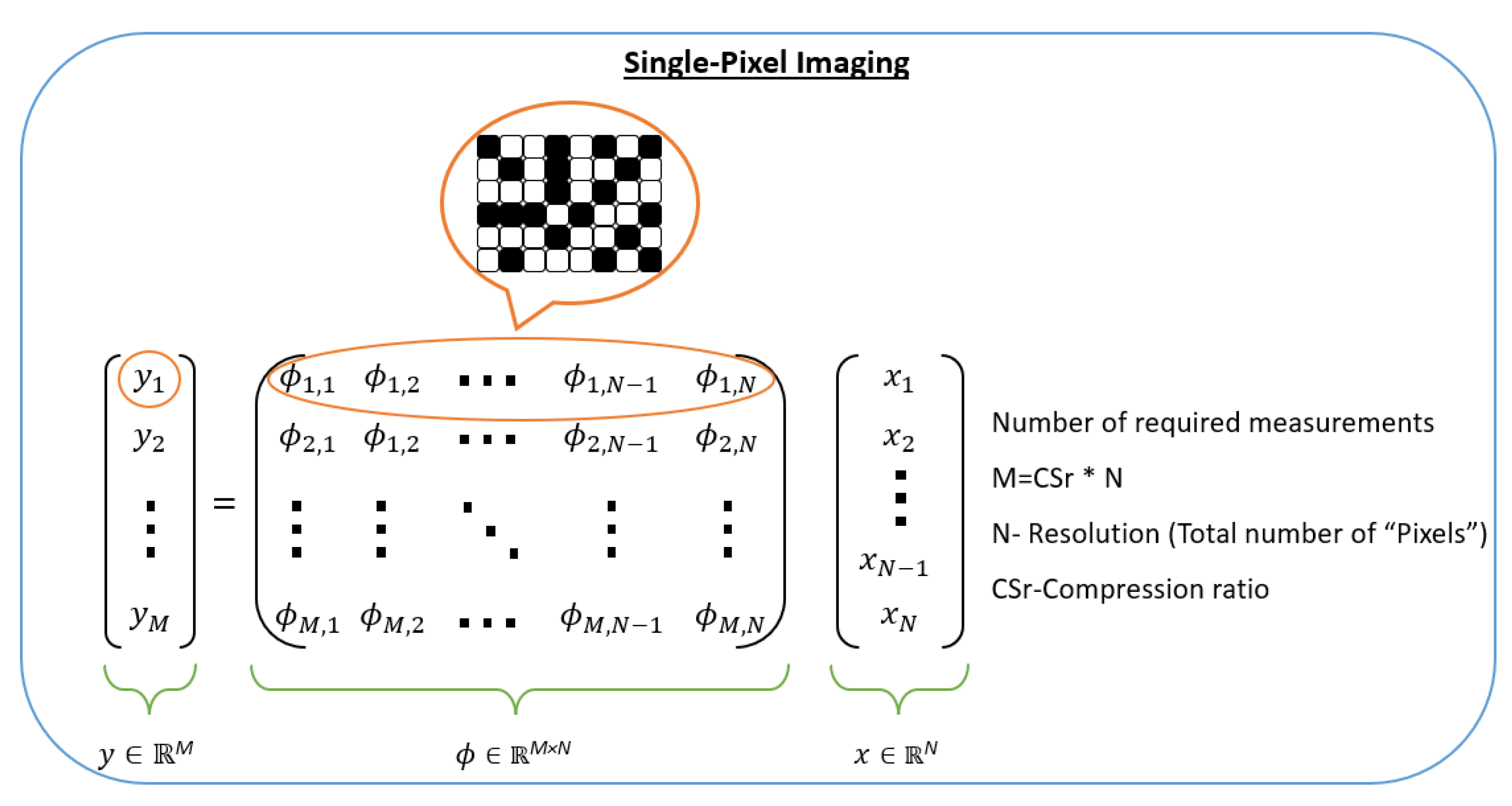
5.1. Single Pixel Imaging
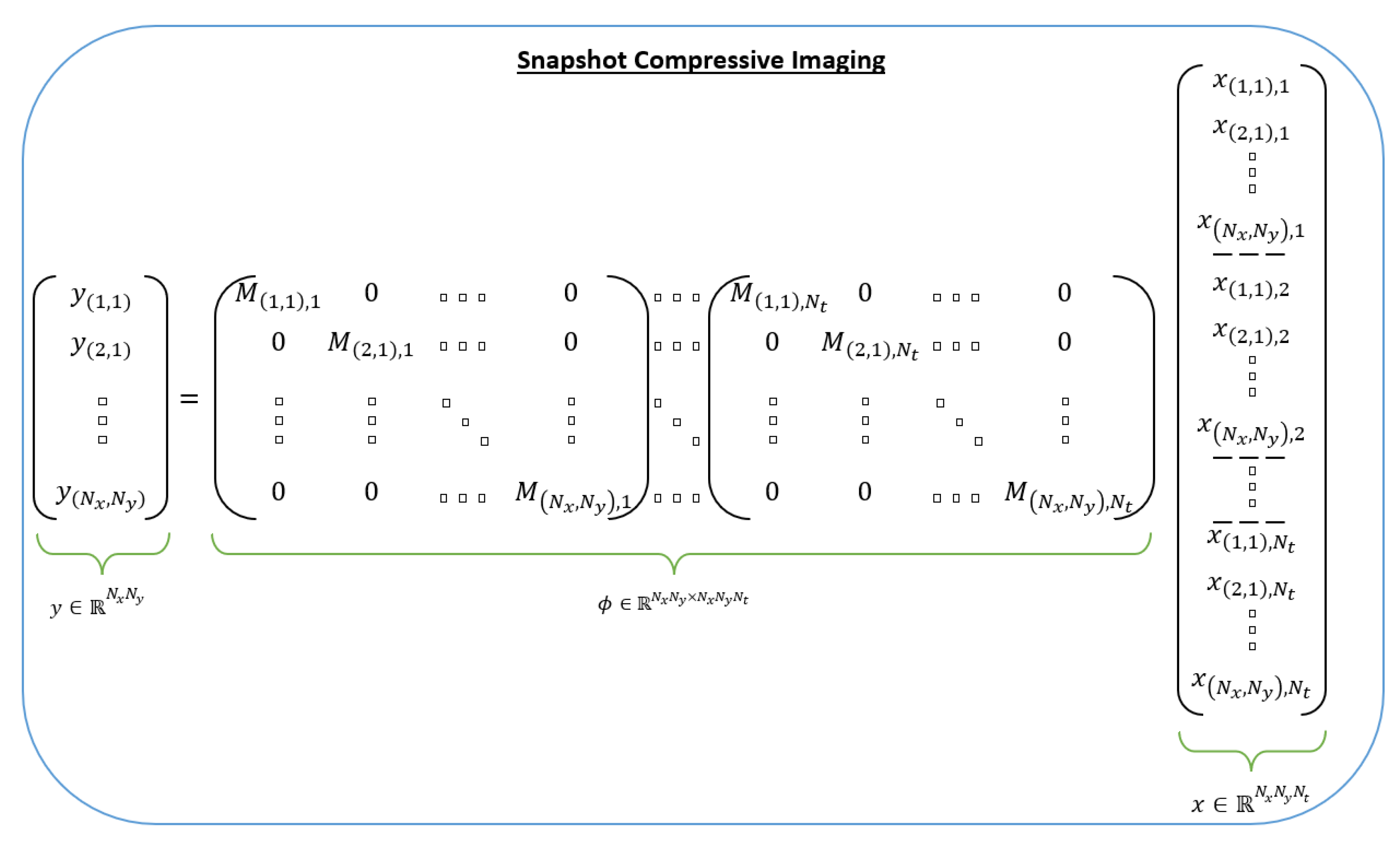
5.2. Video Snapshot Compressive Imaging
6. Comparative Study
6.1. Optimization-Based VCS Algorithms
- The sparsity information: it may not be provided for the reconstruction process
- Noise resistance: It is important to design a recovery algorithm where the measurements are not affected by measurement noise
- Hardware feasibility: low-complexity algorithms can usually be implemented on hardware devices for real-world applications
6.2. Deep Learning-Based VCS Algorithms
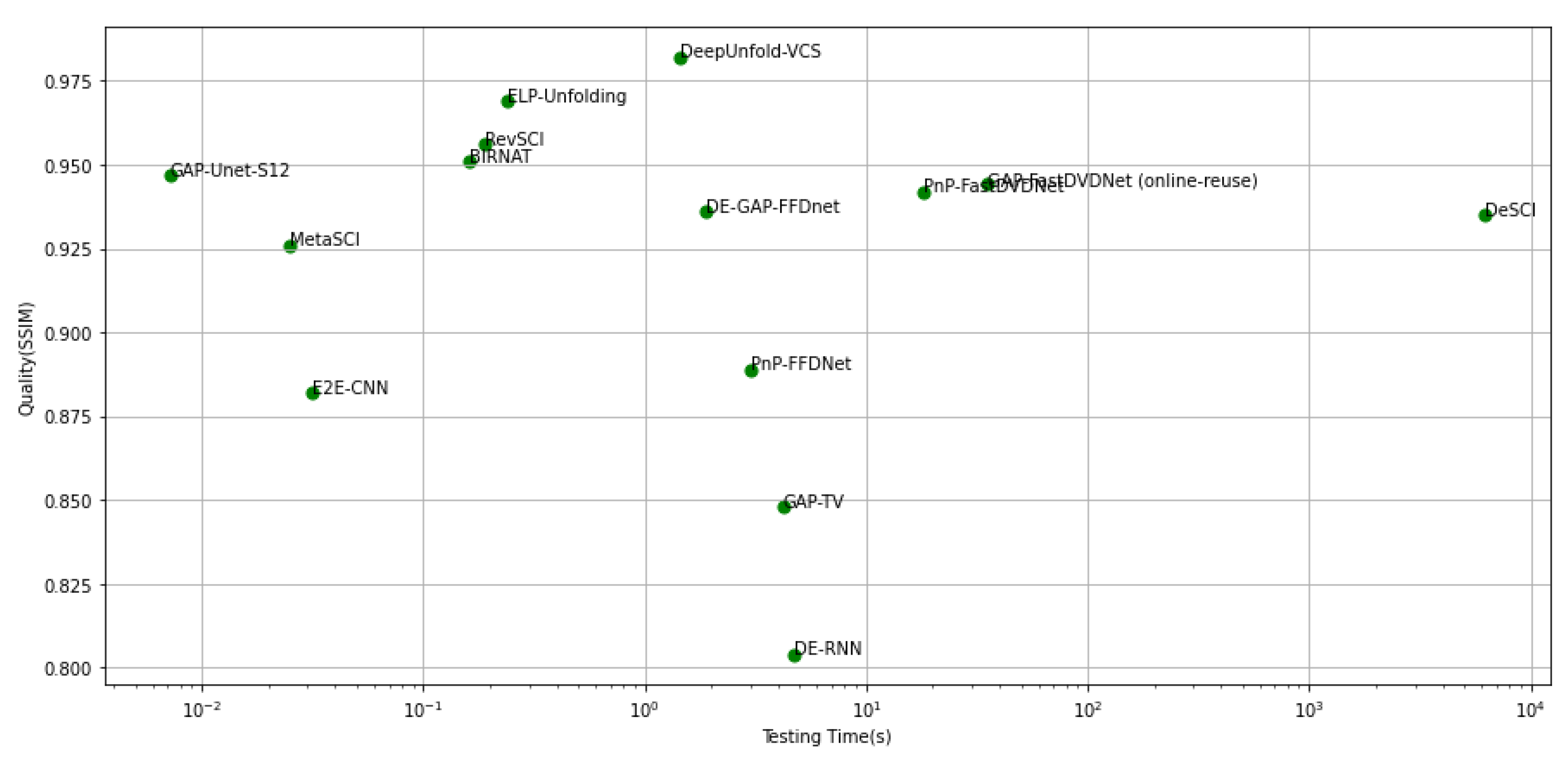
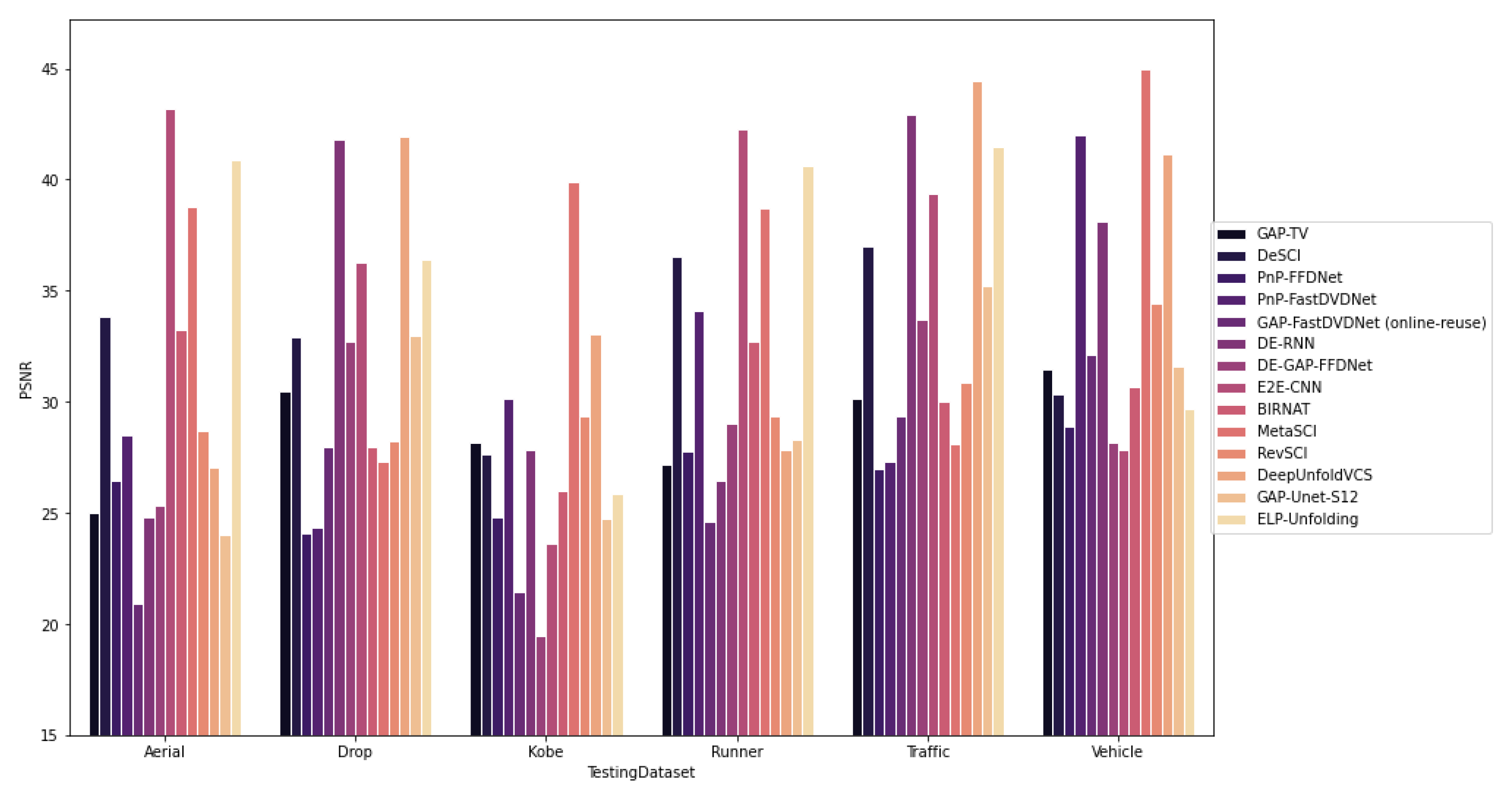
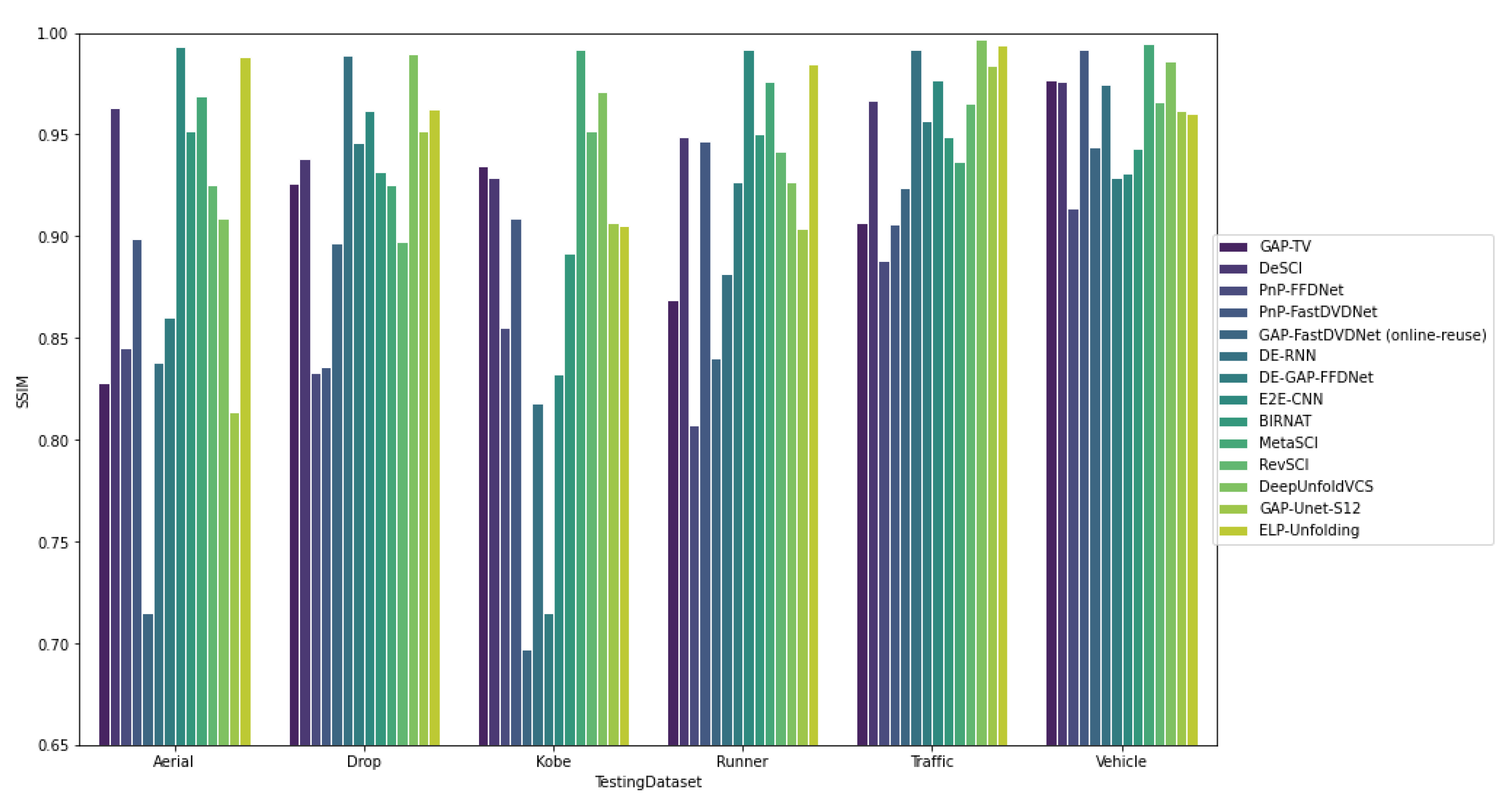
6.2.1. Quantitative Comparison
Training Details
Comparison Metrics
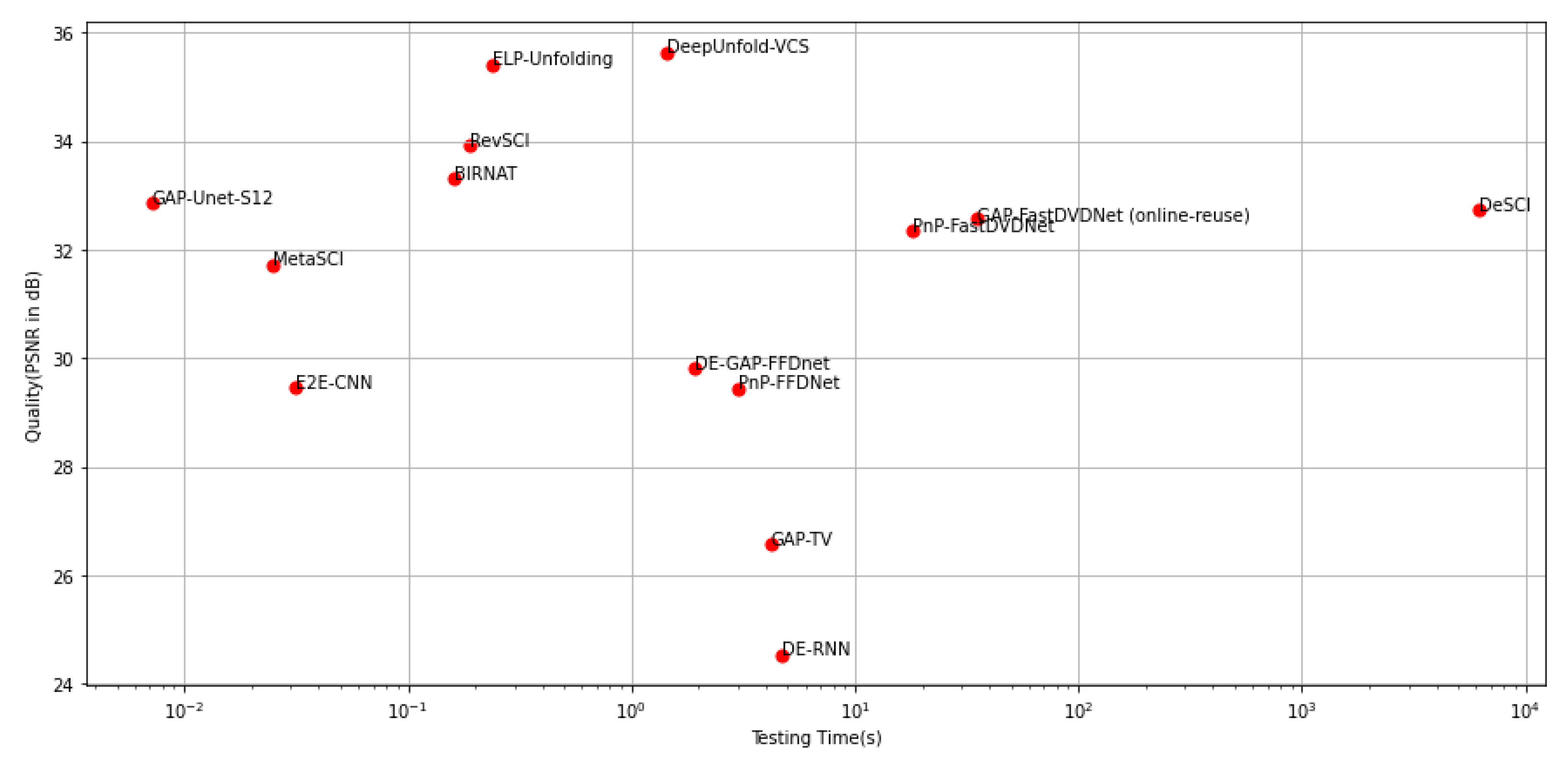
Benchmark Results
6.2.2. Qualitative Comparison
7. Compressive Sensing: Research Challenges and Opportunities
8. Conclusions
Author Contributions
Funding
Conflicts of Interest
References
- Akyildiz, I.F.; Su, W.; Sankarasubramaniam, Y.; Cayirci, E. Wireless sensor networks: A survey. Comput. Netw. 2002, 38, 393–422. [Google Scholar]
- Amarlingam, M.; Mishra, P.K.; Rajalakshmi, P.; Giluka, M.K.; Tamma, B.R. Energy efficient wireless sensor networks utilizing adaptive dictionary in compressed sensing. In Proceedings of the 2018 IEEE 4th World Forum on Internet of Things (WF-IoT), Singapore, 5–8 February 2018; pp. 383–388. [Google Scholar] [CrossRef]
- Donoho, D.L. Compressed sensing. IEEE Trans. Inf. Theory 2006, 52, 1289–1306. [Google Scholar] [CrossRef]
- Duarte, M.F.; Davenport, M.A.; Takhar, D.; Laska, J.N.; Sun, T.; Kelly, K.F.; Baraniuk, R.G. Single-pixel imaging via compressive sampling. IEEE Signal Process. Mag. 2008, 25, 83–91. [Google Scholar] [CrossRef] [Green Version]
- Veeraraghavan, A.; Reddy, D.; Raskar, R. Coded Strobing Photography: Compressive Sensing of High Speed Periodic Videos. IEEE Trans. Pattern Anal. Mach. Intell. 2011, 33, 671–686. [Google Scholar] [CrossRef]
- Wakin, M.; Laska, J.N.; Duarte, M.F.; Baron, D.; Sarvotham, S.; Takhar, D.; Kelly, K.F.; Baraniuk, R.G. Compressive imaging for video representation and coding. In Proceedings of the Picture Coding Symposium, Beijing, China, 24–26 April 2006; pp. 1–6. [Google Scholar]
- Reddy, D.; Veeraraghavan, A.; Chellappa, R. P2C2: Programmable pixel compressive camera for high speed imaging. In Proceedings of the IEEE Conference on Computer Vision and Pattern Recognition (CVPR), Colorado Springs, CO, USA, 20–25 June 2011; pp. 329–336. [Google Scholar]
- Kittle, D.; Choi, K.; Wagadarikar, A.; Brady, D.J. Multiframe image estimation for coded aperture snapshot spectral imagers. Appl. Opt. 2010, 49, 6824–6833. [Google Scholar] [CrossRef]
- Hitomi, Y.; Gu, J.; Gupta, M.; Mitsunaga, T.; Nayar, S.K. Video from a single coded exposure photograph using a learned over-complete dictionary. In Proceedings of the IEEE International Conference on Computer Vision (ICCV), Barcelona, Spain, 6–13 November 2011; pp. 287–294. [Google Scholar]
- Candés, E.J.; Romberg, J.K.; Tao, T. Stable signal recovery from incomplete and inaccurate measurements. Commun. Pure Appl. Math. 2006, 59, 1207–1223. [Google Scholar] [CrossRef] [Green Version]
- Palangi, H.; Ward, R.; Deng, L. Distributed Compressive Sensing: A Deep Learning Approach. IEEE Trans. Signal Process. 2016, 64, 4504–4518. [Google Scholar] [CrossRef] [Green Version]
- Hochreiter, S.; Schmidhuber, J. Long Short-term Memory. Neural Comput. 1997, 9, 1735–1780. [Google Scholar] [CrossRef]
- Candes, E.J.; Plan, Y. A Probabilistic and RIPless Theory of Compressed Sensing. IEEE Trans. Inf. Theory 2011, 57, 7235–7254. [Google Scholar] [CrossRef] [Green Version]
- Nguyen, T.L.; Shin, Y. Deterministic sensing matrices in compressive sensing: A survey. Sci. World J. 2013, 2013, 192795. [Google Scholar] [CrossRef] [Green Version]
- Rousseau, S.; Helbert, D. Compressive Color Pattern Detection Using Partial Orthogonal Circulant Sensing Matrix. IEEE Trans. Image Process. 2020, 29, 670–678. [Google Scholar] [CrossRef] [PubMed]
- Chen, S.S.; Donoho, D.L.; Saunders, M.A. Atomic decomposition by basis pursuit. SIAM J. Sci. Comput. 1998, 20, 33–61. [Google Scholar] [CrossRef]
- Candes, E.J. The restricted isometry property and its implications for compressed sensing. C. R. Math. 2008, 346, 589–592. [Google Scholar] [CrossRef]
- Candes, E.; Tao, T. The Dantzig selector: Statistical estimation when p is much larger than n. Ann. Stat. 2007, 35, 2313–2351. [Google Scholar]
- Beck, A.; Teboulle, M. Fast gradient-based algorithms for constrained total variation image denoising and deblurring problems. IEEE Trans. Image Process. 2009, 18, 2419–2434. [Google Scholar] [CrossRef] [Green Version]
- Combettes, P.L.; Pesquet, J.-C. Proximal splitting methods in signal processing. In Fixed-Point Algorithms for Inverse Problems in Science and Engineering; Springer: New York, NY, USA, 2011; pp. 185–212. [Google Scholar]
- Donoho, D.L.; Maleki, A.; Montanari, A. Message-passing algorithms for compressed sensing. Proc. Natl. Acad. Sci. USA 2009, 106, 18914–18919. [Google Scholar] [CrossRef] [Green Version]
- Figueiredo, M.A.; Nowak, R.D.; Wright, S.J. Gradient projection for sparse reconstruction: Application to compressed sensing and other inverse problems. IEEE J. Sel. Top. Signal Process. 2007, 1, 586–597. [Google Scholar] [CrossRef] [Green Version]
- Mallat, S.G.; Zhang, Z. Matching pursuits with time-frequency dictionaries. IEEE Trans. Signal Process. 1993, 41, 3397–3415. [Google Scholar] [CrossRef] [Green Version]
- Krstulovic, S.; Gribonval, R. MPTK: Matching pursuit made tractable. In Proceedings of the 2006 IEEE International Conference on Acoustics, Speech and Signal Processing (ICASSP), Toulouse, France, 14–19 May 2006; IEEE: Piscataway, NJ, USA, 2006; Volume 3, p. III. [Google Scholar]
- Tropp, J.A.; Gilbert, A.C. Signal recovery from random measurements via orthogonal matching pursuit. IEEE Trans. Inf. Theory 2007, 53, 4655–4666. [Google Scholar] [CrossRef] [Green Version]
- Donoho, D.L.; Tsaig, Y.; Drori, I.; Starck, J.-L. Sparse solution of underdetermined systems of linear equations by stagewise orthogonal matching pursuit. IEEE Trans. Inf. Theory 2012, 58, 1094–1121. [Google Scholar] [CrossRef]
- Needell, D.; Vershynin, R. Uniform uncertainty principle and signal recovery via regularized orthogonal matching pursuit. Found. Comp. Math. 2009, 9, 317–334. [Google Scholar] [CrossRef]
- Tropp, J. Greed is good: Algorithmic results for sparse approximation. IEEE Trans. Inf. Theory 2004, 50, 2231–2242. [Google Scholar] [CrossRef] [Green Version]
- Needell, D.; Tropp, J.A. CoSaMP: Iterative signal recovery from incomplete and inaccurate samples. Appl. Comput. Harmon. Anal. 2009, 26, 301–321. [Google Scholar] [CrossRef] [Green Version]
- Dai, W.; Milenkovic, O. Subspace pursuit for compressive sensing signal reconstruction. IEEE Trans. Inf. Theory 2009, 55, 2230–2249. [Google Scholar] [CrossRef] [Green Version]
- Liu, E.; Temlyakov, V.N. The orthogonal super greedy algorithm and applications in compressed sensing. IEEE Trans. Inf. Theory 2012, 58, 2040–2047. [Google Scholar] [CrossRef]
- Xuan, Y.; Yang, C. 2Ser-Vgsr-Net: A Two-Stage Enhancement Reconstruction Based On Video Group Sparse Representation Network For Compressed Video Sensing. In Proceedings of the 2020 IEEE International Conference on Multimedia and Expo (ICME), London, UK, 6–10 July 2020; pp. 1–6. [Google Scholar] [CrossRef]
- Mousavi, A.; Patel, A.B.; Baraniuk, R.G. A deep learning approach to structured signal recovery. In Proceedings of the 2015 53rd Annual Allerton Conference on Communication, Control, and Computing (Allerton), Monticello, IL, USA, 29 September–2 October 2015; pp. 1336–1343. [Google Scholar] [CrossRef] [Green Version]
- Kulkarni, K.; Lohit, S.; Turaga, P.; Kerviche, R.; Ashok, A. ReconNet: Non-iterative reconstruction of images from compressively sensed measurements. In Proceedings of the IEEE Conference on Computer Vision and Pattern Recognition (CVPR), Las Vegas, NV, USA, 27–30 June 2016; pp. 449–458. [Google Scholar]
- Yao, H.T.; Dai, F.; Zhang, S.L.; Zhang, Y.D.; Tian, Q.; Xu, C.S. DR2 -Net: Deep residual reconstruction network for image compressive sensing. Neurocomputing 2019, 359, 483–493. [Google Scholar] [CrossRef] [Green Version]
- Zhang, J.; Ghanem, B. ISTA-Net: Interpretable optimization-inspired deep network for image compressive sensing. In Proceedings of the IEEE Conference on Computer Vision and Pattern Recognition (CVPR), Salt Lake City, UT, USA, 18–23 June 2018; pp. 1828–1837. [Google Scholar]
- Ito, D.; Takabe, S.; Wadayama, T. Trainable ISTA for Sparse Signal Recovery. IEEE Trans. Signal Process. 2019, 67, 3113–3125. [Google Scholar] [CrossRef] [Green Version]
- Su, H.; Bao, Q.; Chen, Z. ADMM–Net: A Deep Learning Approach for Parameter Estimation of Chirp Signals under Sub-Nyquist Sampling. IEEE Access 2020, 8, 75714–75727. [Google Scholar] [CrossRef]
- Shi, W.; Jiang, F.; Liu, S.; Zhao, D. Image Compressed Sensing Using Convolutional Neural Network. IEEE Trans. Image Process. 2020, 29, 375–388. [Google Scholar] [CrossRef]
- Canh, T.N.; Jeon, B. Multi-Scale Deep Compressive Sensing Network. In Proceedings of the 2018 IEEE Visual Communications and Image Processing (VCIP), Taichung, Taiwan, 9–12 December 2018; pp. 1–4. [Google Scholar] [CrossRef] [Green Version]
- Canh, T.N.; Jeon, B. Difference of Convolution for Deep Compressive Sensing. In Proceedings of the 2019 IEEE International Conference on Image Processing (ICIP), Taipei, Taiwan, 22–25 September 2019; pp. 2105–2109. [Google Scholar] [CrossRef]
- Shi, W.; Jiang, F.; Liu, S.; Zhao, D. Scalable Convolutional Neural Network for Image Compressed Sensing. In Proceedings of the 2019 IEEE/CVF Conference on Computer Vision and Pattern Recognition (CVPR), Long Beach, CA, USA, 15–20 June 2019; pp. 12282–12291. [Google Scholar] [CrossRef]
- Yang, J.; Yuan, X.; Liao, X.; Llull, P.; Brady, D.J.; Sapiro, G.; Carin, L. Video compressive sensing using Gaussian mixture models. IEEE Trans. Image Process. 2014, 23, 4863–4878. [Google Scholar] [CrossRef]
- Yuan, X. Generalized alternating projection based total variation minimization for compressive sensing. In Proceedings of the IEEE International Conference on Image Processing (ICIP), Phoenix, AZ, USA, 25–28 September 2016; pp. 2539–2543. [Google Scholar]
- Iliadis, M.; Spinoulas, L.; Katsaggelos, A.K. Deep fully-connected networks for video compressive sensing. Digit. Signal Process. 2018, 72, 9–18. [Google Scholar] [CrossRef] [Green Version]
- Horé, A.; Ziou, D. Image Quality Metrics: PSNR vs. SSIM. In Proceedings of the 2010 20th International Conference on Pattern Recognition, Istanbul, Turkey, 23–26 August 2010; pp. 2366–2369. [Google Scholar] [CrossRef]
- Higham, C.F.; Murray-Smith, R.; Padgett, M.J.; Edgar, M.P. Deep learning for realtime single-pixel video. Sci. Rep. 2018, 8, 2369. [Google Scholar] [CrossRef] [PubMed] [Green Version]
- Qiao, M.; Meng, Z.; Ma, J.; Yuan, X. Deep learning for video compressive sensing. APL Photonics 2020, 5, 030801. [Google Scholar] [CrossRef]
- Bioucas-Dias, J.M.; Figueiredo, M.A.T. A New TwIST: Two-Step Iterative Shrinkage/Thresholding Algorithms for Image Restoration. IEEE Trans. Image Process. 2007, 16, 2992–3004. [Google Scholar] [CrossRef] [PubMed] [Green Version]
- Zhang, L.; Lam, E.Y.; Ke, J. Temporal compressive imaging reconstruction based on a 3D-CNN network. Opt. Express 2022, 30, 3577–3591. [Google Scholar] [CrossRef]
- Zheng, S.; Yang, X.; Yuan, X. Two-Stage is Enough: A Concise Deep Unfolding Reconstruction Network for Flexible Video Compressive Sensing. arXiv 2022, arXiv:2201.05810. [Google Scholar]
- Zhao, C.; Ma, S.; Zhang, J.; Xiong, R.; Gao, W. Video compressive sensing reconstruction via reweighted residual sparsity. IEEE Trans. Circuits Syst. Video Technol. 2017, 27, 1182–1195. [Google Scholar] [CrossRef]
- Xu, K.; Ren, F. CSVideoNet: A real-time end-to-end learning framework for high-frame-rate video compressive sensing. In Proceedings of the 2018 IEEE Winter Conference on Applications of Computer Vision (WACV), Lake Tahoe, NV, USA, 12–15 March 2018; pp. 1680–1688. [Google Scholar]
- Albawi, S.; Mohammed, T.A.; Al-Zawi, S. Understanding of a convolutional neural network. In Proceedings of the 2017 International Conference on Engineering and Technology (ICET), Antalya, Turkey, 21–23 August 2017; pp. 1–6. [Google Scholar] [CrossRef]
- Chen, H.; Salman Asif, M.; Sankaranarayanan, A.C.; Veeraraghavan, A. FPA-CS: Focal plane array-based compressive imaging in short-wave infrared. In Proceedings of the 2015 IEEE Conference on Computer Vision and Pattern Recognition (CVPR), Boston, MA, USA, 7–12 June 2015; pp. 2358–2366. [Google Scholar] [CrossRef] [Green Version]
- Wang, J.; Gupta, M.; Sankaranarayanan, A.C. LiSens—A Scalable Architecture for Video Compressive Sensing. In Proceedings of the 2015 IEEE International Conference on Computational Photography (ICCP), Houston, TX, USA, 24–26 April 2015; pp. 1–9. [Google Scholar] [CrossRef] [Green Version]
- Xiong, T.; Rattray, J.; Zhang, J.; Thakur, C.S.; Chin, S.; Tran, T.D.; Etienne-Cummings, R. Spatiotemporal compressed sensing for video compression. In Proceedings of the 2017 IEEE 60th International Midwest Symposium on Circuits and Systems (MWSCAS), Boston, MA, USA, 6–9 August 2017. [Google Scholar]
- Wang, X.; Zhang, J.; Xiong, T.; Tran, T.D.; Chin, S.P.; Etienne-Cummings, R. Using deep learning to extract scenery information in real time spatiotemporal compressed sensing. In Proceedings of the 2018 IEEE International Symposium on Circuits and Systems (ISCAS), Florence, Italy, 27–30 May 2018; pp. 1–4. [Google Scholar]
- Lam, D.; Wunsch, D. Video compressive sensing with 3-D wavelet and 3-D noiselet. In Proceedings of the 19th IEEE International Conference on Image Processing (ICIP ’12), Orlando, FL, USA, 30 September–3 October 2012. [Google Scholar] [CrossRef]
- Ji, S.; Xu, W.; Yang, M.; Yu, K. 3D convolutional neural networks for human action recognition. IEEE Trans. Pattern Anal. Mach. Intell. 2013, 35, 221–231. [Google Scholar] [CrossRef] [Green Version]
- Zhao, Z.; Xie, X.; Liu, W.; Pan, Q. A hybrid-3D convolutional network for video compressive sensing. IEEE Access 2020, 8, 20503–20513. [Google Scholar] [CrossRef]
- Tran, D.; Bourdev, L.; Fergus, R.; Torresani, L.; Paluri, M. Learning spatiotemporal features with 3D convolutional networks. In Proceedings of the IEEE International Conference on Computer Vision (ICCV), Santiago, Chile, 7–13 December 2015; pp. 4489–4497. [Google Scholar]
- Wei, Z.; Yang, C.; Xuan, Y. Efficient Video Compressed Sensing Reconstruction via Exploiting Spatial-Temporal Correlation with Measurement Constraint. In Proceedings of the 2021 IEEE International Conference on Multimedia and Expo (ICME), Shenzhen, China, 5–9 July 2021; pp. 1–6. [Google Scholar]
- Rousset, F.; Ducros, N.; Farina, A.; Valentini, G.; D’Andrea, C.; Peyrin, F. Adaptive Basis Scan by Wavelet Prediction for Single-pixel Imaging. IEEE Trans. Comput. Imaging 2016, 3, 36–46. [Google Scholar] [CrossRef] [Green Version]
- Baraniuk, R.G.; Goldstein, T.; Sankaranarayanan, A.C.; Studer, C.; Veeraraghavan, A.; Wakin, M.B. Compressive video sensing: Algorithms, architectures, and applications. IEEE Signal Process. Mag. 2017, 34, 52–66. [Google Scholar] [CrossRef]
- Mur, A.L.; Peyrin, F.; Ducros, N. Recurrent Neural Networks for Compressive Video Reconstruction. In Proceedings of the IEEE 17th International Symposium on Biomedical Imaging (ISBI), Iowa City, IA, USA, 3–7 April 2020; pp. 1651–1654. [Google Scholar]
- Ducros, N.; Lorente Mur, A.; Peyrin, F. A completion network for reconstruction from compressed acquisition. In Proceedings of the 2020 IEEE 17th International Symposium on Biomedical Imaging (ISBI), Iowa City, IA, USA, 3–7 April 2020; pp. 619–623. [Google Scholar]
- Yuan, X.; Brady, D.; Katsaggelos, A.K. Snapshot compressive imaging: Theory, algorithms and applications. IEEE Signal Process. Mag. 2020, 38, 65–88. [Google Scholar] [CrossRef]
- Llull, P.; Liao, X.; Yuan, X.; Yang, J.; Kittle, D.; Carin, L.; Sapiro, G.; Brady, D.J. Coded aperture compressive temporal imaging. Opt. Express 2013, 21, 10526–10545. [Google Scholar] [CrossRef] [PubMed] [Green Version]
- Koller, R.; Schmid, L.; Matsuda, N.; Niederberger, T.; Spinoulas, L.; Cossairt, O.; Schuster, G.; Katsaggelos, A.K. High spatio-temporal resolution video with compressed sensing. Opt. Express 2015, 23, 15992–16007. [Google Scholar] [CrossRef]
- Sun, Y.; Yuan, X.; Pang, S. Compressive high-speed stereo imaging. Opt. Express 2017, 25, 18182–18190. [Google Scholar] [CrossRef]
- Jalali, S.; Yuan, X. Snapshot compressed sensing: Performance bounds and algorithms. IEEE Trans. Inf. Theory 2019, 65, 8005–8024. [Google Scholar] [CrossRef] [Green Version]
- Liu, Y.; Yuan, X.; Suo, J.; Brady, D.J.; Dai, Q. Rank Minimization for Snapshot Compressive Imaging. IEEE Trans. Pattern Anal. Mach. Intell. 2019, 41, 2990–3006. [Google Scholar] [CrossRef] [Green Version]
- Yuan, X.; Liu, Y.; Suo, J.; Dai, Q. Plug-and-Play Algorithms for Large-Scale Snapshot Compressive Imaging. In Proceedings of the 2020 IEEE/CVF Conference on Computer Vision and Pattern Recognition (CVPR), Seattle, WA, USA, 13–19 June 2020; pp. 1444–1454. [Google Scholar] [CrossRef]
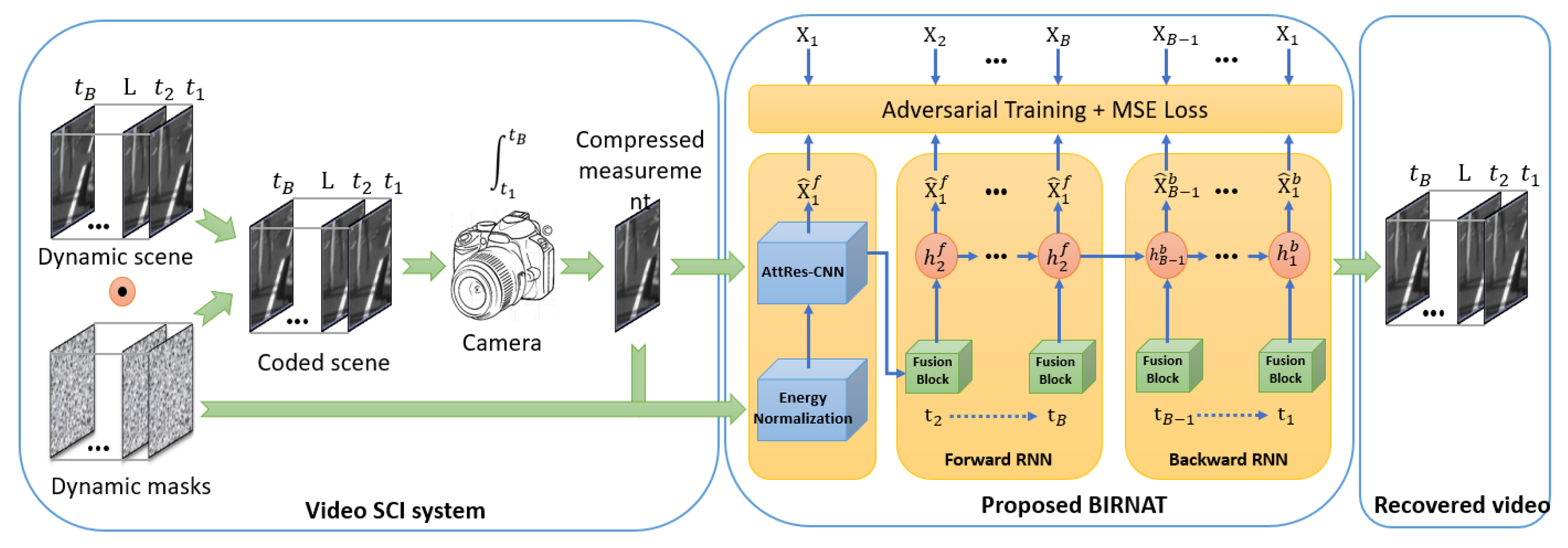
- Cheng, Z.; Lu, R.; Wang, Z.; Zhang, H.; Chen, B.; Meng, Z.; Yuan, X. BIRNAT: Bidirectional recurrent neural networks with adversarial training for video snapshot compressive imaging. In Proceedings of the European Conference on Computer Vision (ECCV), Glasgow, UK, 23–28 August 2020. [Google Scholar]
- Meng, Z.; Jalali, S.; Yuan, X. Gap-net for snapshot compressive imaging. arXiv 2020, arXiv:2012.08364. [Google Scholar]
- Yuan, X.; Pu, Y. Parallel lensless compressive imaging via deep convolutional neural networks. Opt. Express 2018, 26, 1962–1977. [Google Scholar] [CrossRef]
- Ma, J.; Liu, X.; Shou, Z.; Yuan, X. Deep tensor admm-net for snapshot compressive imaging. In Proceedings of the IEEE/CVF Conference on Computer Vision (ICCV), Seoul, Korea, 27 October–2 November 2019. [Google Scholar]
- Iliadis, M.; Spinoulas, L.; Katsaggelos, A.K. Deepbinarymask: Learning a binary mask for video compressive sensing. Digit. Signal Process. 2020, 96, 102591. [Google Scholar] [CrossRef]
- He, K.; Zhang, X.; Ren, S.; Sun, J. Deep residual learning for image recognition. In Proceedings of the CVPR, Las Vegas, NV, USA, 27–30 June 2016. [Google Scholar]
- Vaswani, A.; Shazeer, N.; Parmar, N.; Uszkoreit, J.; Jones, L.; Gomez, A.N.; Kaiser, L.; Polosukhin, I. Attention is all you need. In Advances in Neural Information Processing Systems 30; Guyon, I., Luxburg, U.V., Bengio, S., Wallach, H., Fergus, R., Vishwanathan, S., Garnett, R., Eds.; Curran Associates, Inc.: Red Hook, NY, USA, 2017; pp. 5998–6008. [Google Scholar]
- Cheng, Z.; Chen, B.; Liu, G.; Zhang, H.; Lu, R.; Wang, Z.; Yuan, X. Memory-efficient network for large-scale video compressive sensing. In Proceedings of the IEEE/CVF Conference on Computer Vision and Pattern Recognition (CVPR), Nashville, TN, USA, 20–25 June 2021. [Google Scholar]
- Wang, Z.; Zhang, H.; Cheng, Z.; Chen, B.; Yuan, X. Metasci: Scalable and adaptive reconstruction for video compressive sensing. In Proceedings of the IEEE/CVF Conference on Computer Vision and Pattern Recognition (CVPR), Nashville, TN, USA, 20–25 June 2021. [Google Scholar]
- Yang, C.; Zhang, S.; Yuan, X. Ensemble learning priors unfolding for scalable Snapshot Compressive Sensing. arXiv 2022, arXiv:2201.10419. [Google Scholar]
- Wu, Z.; Yang, C.; Su, X.; Yuan, X. Adaptive Deep PnP Algorithm for Video Snapshot Compressive Imaging. arXiv 2022, arXiv:2201.05483. [Google Scholar]
- Zhao, Y.; Zheng, S.; Yuan, X. Deep Equilibrium Models for Video Snapshot Compressive Imaging. arXiv 2022, arXiv:2201.06931. [Google Scholar]
- Pont-Tuset, J.; Perazzi, F.; Caelles, S.; Arbelaez, P.; Sorkine-Hornung, A.; Gool, L.V. The 2017 DAVIS challenge on video object segmenta tion. arXiv 2017, arXiv:1704.00675. [Google Scholar]
- Yuan, X.; Liu, Y.; Suo, J.; Durand, F.; Dai, Q. Plug-and-play algorithms for video snapshot compressive imaging. arXiv 2021, arXiv:2101.04822. [Google Scholar]
- Liu, S.; Liu, L.; Tang, J.; Yu, B.; Wang, Y.; Shi, W. Edge computing for autonomous driving: Opportunities and challenges. Proc. IEEE 2019, 107, 1697–1716. [Google Scholar] [CrossRef]
- Lu, S.; Yuan, X.; Shi, W. An integrated framework for compressive imaging processing on CAVs. In Proceedings of the ACM/IEEE Symposium on Edge Computing (SEC), San Jose, CA, USA, 12–14 November 2020. [Google Scholar]


| Algorithms | Min. Number of Measurements | Complexity | No Requirement of Sparsity Information | Noise Resistance | Hardware Implementation |
|---|---|---|---|---|---|
| Basis Pursuit | ✓ | ||||
| OMP | ✓ | ✓ | |||
| StOMP | ✓ | ✓ | |||
| ROMP | ✓ | ✓ | |||
| CoSaMP | ✓ | ✓ | |||
| Subspace Pursuits | ✓ | ✓ |
| Algorithms | Year | Aerial | Drop | Kobe | Runner | Traffic | Vehicle | Average | Time |
|---|---|---|---|---|---|---|---|---|---|
| GAP-TV [44] | 2016 | 25.03 | 33.81 | 26.45 | 28.48 | 20.90 | 24.82 | 26.58 | 4.2 |
| 0.828 | 0.963 | 0.845 | 0.899 | 0.715 | 0.838 | 0.848 | |||
| DeSCI [73] | 2019 | 25.33 | 43.22 | 33.25 | 38.76 | 28.72 | 27.04 | 32.72 | 6180 |
| 0.860 | 0.993 | 0.952 | 0.969 | 0.925 | 0.909 | 0.935 | |||
| PnP-FFDNet [74] | 2020 | 24.02 | 40.87 | 30.47 | 32.88 | 24.08 | 24.32 | 29.44 | 3.0 |
| 0.814 | 0.988 | 0.926 | 0.938 | 0.833 | 0.836 | 0.889 | |||
| Pnp-FastDVDNet [88] | 2021 | 27.98 | 41.82 | 32.73 | 36.29 | 27.95 | 27.32 | 32.35 | 18 |
| 0.897 | 0.989 | 0.946 | 0.962 | 0.932 | 0.925 | 0.942 | |||
| GAP-FastDVDNet(online) [85] | 2022 | 28.24 | 41.95 | 32.95 | 36.41 | 28.16 | 27.64 | 32.56 | 35 |
| 0.897 | 0.989 | 0.951 | 0.962 | 0.934 | 0.928 | 0.944 | |||
| DE-RNN [86] | 2022 | 24.83 | 30.16 | 21.46 | 27.85 | 19.47 | 23.65 | 24.53 | 4.68 |
| 0.855 | 0.909 | 0.697 | 0.818 | 0.715 | 0.832 | 0.804 | |||
| DE-GAP-FFDnet [86] | 2022 | 26.02 | 39.89 | 29.32 | 33.06 | 24.71 | 25.85 | 29.81 | 1.90 |
| 0.892 | 0.992 | 0.952 | 0.971 | 0.907 | 0.905 | 0.936 | |||
| E2E-CNN [48] | 2020 | 27.18 | 36.56 | 27.79 | 34.12 | 24.62 | 26.43 | 29.45 | 0.0312 |
| 0.869 | 0.949 | 0.807 | 0.947 | 0.840 | 0.882 | 0.882 | |||
| BIRNAT [75] | 2020 | 28.99 | 42.28 | 32.71 | 38.70 | 29.33 | 27.84 | 33.31 | 0.16 |
| 0.927 | 0.992 | 0.950 | 0.976 | 0.942 | 0.927 | 0.951 | |||
| MetaSCI [83] | 2021 | 28.31 | 40.61 | 30.12 | 37.02 | 26.95 | 27.33 | 31.72 | 0.025 |
| 0.904 | 0.985 | 0.907 | 0.967 | 0.888 | 0.906 | 0.926 | |||
| RevSCI [82] | 2021 | 29.35 | 42.93 | 33.72 | 39.40 | 30.02 | 28.12 | 33.92 | 0.19 |
| 0.924 | 0.992 | 0.957 | 0.977 | 0.949 | 0.937 | 0.956 | |||
| DeepUnfold-VCS [51] | 2022 | 30.86 | 44.43 | 35.24 | 41.47 | 31.45 | 30.32 | 35.63 | 1.43 |
| 0.965 | 0.997 | 0.984 | 0.994 | 0.977 | 0.976 | 0.982 | |||
| GAP-Unet-S12 [76] | 2020 | 28.88 | 42.02 | 32.09 | 38.12 | 28.19 | 27.83 | 32.86 | 0.0072 |
| 0.914 | 0.992 | 0.944 | 0.975 | 0.929 | 0.931 | 0.947 | |||
| ELP-Unfolding [84] | 2022 | 30.68 | 44.99 | 34.41 | 41.16 | 31.58 | 29.65 | 35.41 | 0.24 |
| 0.943 | 0.995 | 0.966 | 0.986 | 0.962 | 0.960 | 0.969 |
| Classification Type | Category | Traditional/DL | Algorithm’s Class | Examples | Advantages | Limitations |
|---|---|---|---|---|---|---|
| Sampling strategy | Temporal VCS | Traditional | GMM based | GMM [43] | Parallel processing can be used, good quality performances, flexibility | Too computationally slow, slow reconstruction process, use only the temporal domain to compress the video |
| TV based | GAP-TV [44] | |||||
| DL | Deep fully connected network for VCS [45], DCAN [47], E2E-CNN [48] | |||||
| Spatial VCS | Traditional | Reweighted residual sparsity | VCS-RRS [52] | Good performances, flexibility | use only the spatial domain to compress the video, Low scalability | |
| Extended architectures of SPC | FPA-CS [55], LiSens [56] | High spatial resolution, flexibility | Expensive | |||
| DL | RNN based | CSVideoNet [53], SDA-CS [33] | ||||
| CNN based | ReconNet [34] | |||||
| Spatio-temporal VCS | Traditional | ST-approach [57] | Sample the temporal and spatial dimension simultaneously | Huge computational cost | ||
| TV based | 3D-Wavelet and 3D-Noiselet approach [59] | |||||
| DL | CNN based | [58,60,61,62] |
| Classification Type | Category | Traditional/DL | Algorithm’s Class | Examples | Advantages | Limitations |
|---|---|---|---|---|---|---|
| Modulation strategy | Video Snapshot Compressive Imaging | Traditional | Sparse based | Low-Cost Compressive Sensing for Color Video and Depth | Good flexibility | Very slow algorithms |
| TV based | TwIST [49], GAP-TV [44] | |||||
| GMM | GMM (Off-line training) [43] | |||||
| Dictionary Learning | 3D K-SVD | |||||
| DL | Deep Unfolding | ADMM-Net [78], BIRNAT [75], RevSCI-Net [82], MetaSCI-Net [83] | Good reconstruction quality, Fast algorithms, less GPU memory consumption (RevSCI-Net, MetaSCI-Net) | Less flexible, Not robust to real data noise, huge GPU memory consumption (BIRNAT, ADMM-Net) | ||
| Plug and Play | [48,74] | Good trade-off between accuracy, speed and flexibility | The training phase can be slow | |||
| End-to-End | E2E-CNN [48] | Fast algorithms | Low flexibility | |||
| Single pixel Cameras | Traditional | -regularized approach | Good quality | Slow | ||
| -regularized approach | Fast | Less good quality | ||||
| DL | RNN based | [66] | Good reconstruction quality, | Huge computational time | ||
| CNN based | [67] | Faster training | Huge memory consumption | |||
| Auto-encoder based | [47] |
Publisher’s Note: MDPI stays neutral with regard to jurisdictional claims in published maps and institutional affiliations. |
© 2022 by the authors. Licensee MDPI, Basel, Switzerland. This article is an open access article distributed under the terms and conditions of the Creative Commons Attribution (CC BY) license (https://creativecommons.org/licenses/by/4.0/).
Share and Cite
Saideni, W.; Helbert, D.; Courreges, F.; Cances, J.-P. An Overview on Deep Learning Techniques for Video Compressive Sensing. Appl. Sci. 2022, 12, 2734. https://doi.org/10.3390/app12052734
Saideni W, Helbert D, Courreges F, Cances J-P. An Overview on Deep Learning Techniques for Video Compressive Sensing. Applied Sciences. 2022; 12(5):2734. https://doi.org/10.3390/app12052734
Chicago/Turabian StyleSaideni, Wael, David Helbert, Fabien Courreges, and Jean-Pierre Cances. 2022. "An Overview on Deep Learning Techniques for Video Compressive Sensing" Applied Sciences 12, no. 5: 2734. https://doi.org/10.3390/app12052734