LW-FIRE: A Lightweight Wildfire Image Classification with a Deep Convolutional Neural Network

Abstract

Analysis of reports published by the leading national centers for monitoring wildfires and other emergencies revealed that the devastation caused by wildfires has increased by 2.96-fold when compared to a decade earlier. The reports show that the total number of wildfires is declining; however, their impact on the wildlife appears to be more devastating. In recent years, deep neural network models have demonstrated state-of-the-art accuracy on many computer vision tasks. In this paper, we describe the design and implementation of a lightweight wildfire image classification model (LW-FIRE) based on convolutional neural networks. We explore different ways of using the existing dataset to efficiently train a deep convolutional neural network. We also propose a new method for dataset transformation to increase the number of samples in the dataset and improve the accuracy and generalization of the deep learning model. Experimental results show that the proposed model outperforms the state-of-the-art methods, and is suitable for real-time classification of wildfire images.

1. Introduction

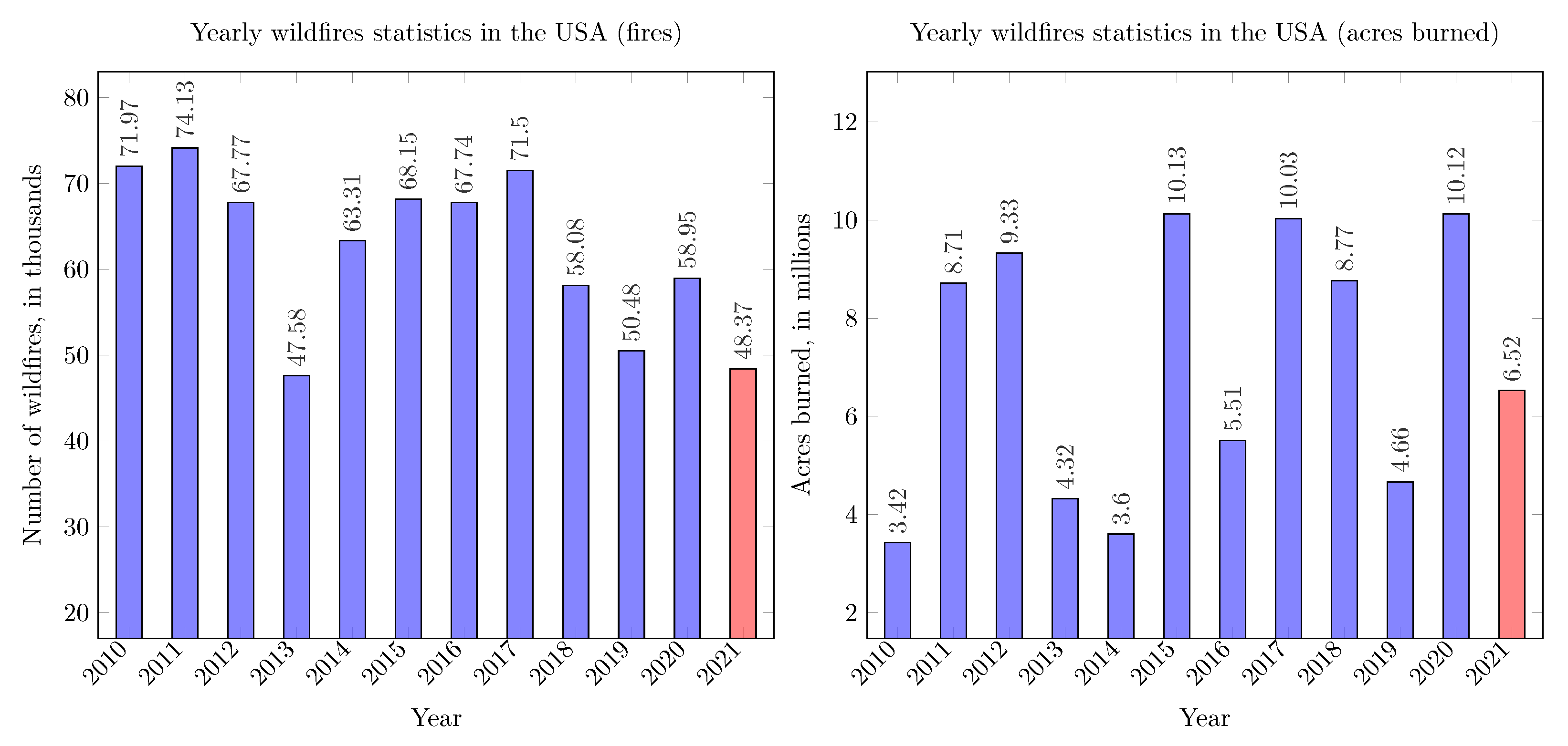
The recent reports from the National Interagency Fire Center (NIFC) show that the number of wildfires is decreasing on an annual level in the USA [1,2,3]. At the same time, the impact and devastation caused by wildfires are becoming greater as evidenced by the increasing average number of acres burned by a single wildfire. The total number of wildfires and the total number of acres burned annually over the period of the last 12 years, including the data which are partially available for the year 2021, are shown in Figure 1. In the 2020 report, 58,950 wildfires were recorded, along with 10.12 million acres of land burned as a consequence of wildfires. A decade earlier, 71,970 wildfires were recorded along with 3.42 million acres of land burned. This data shows an alarming increase in the total burned land area (2.96-fold increase), and it also shows that the overall level of devastation caused by a single wildfire has increased. On average, a single wildfire in 2020 burned 3.61 times more land than in 2010. From 2010 to 2020, on average, 63,605 wildfires per year were recorded, while 7.1 million acres per year were burned (the size of Maryland or Hawaii).

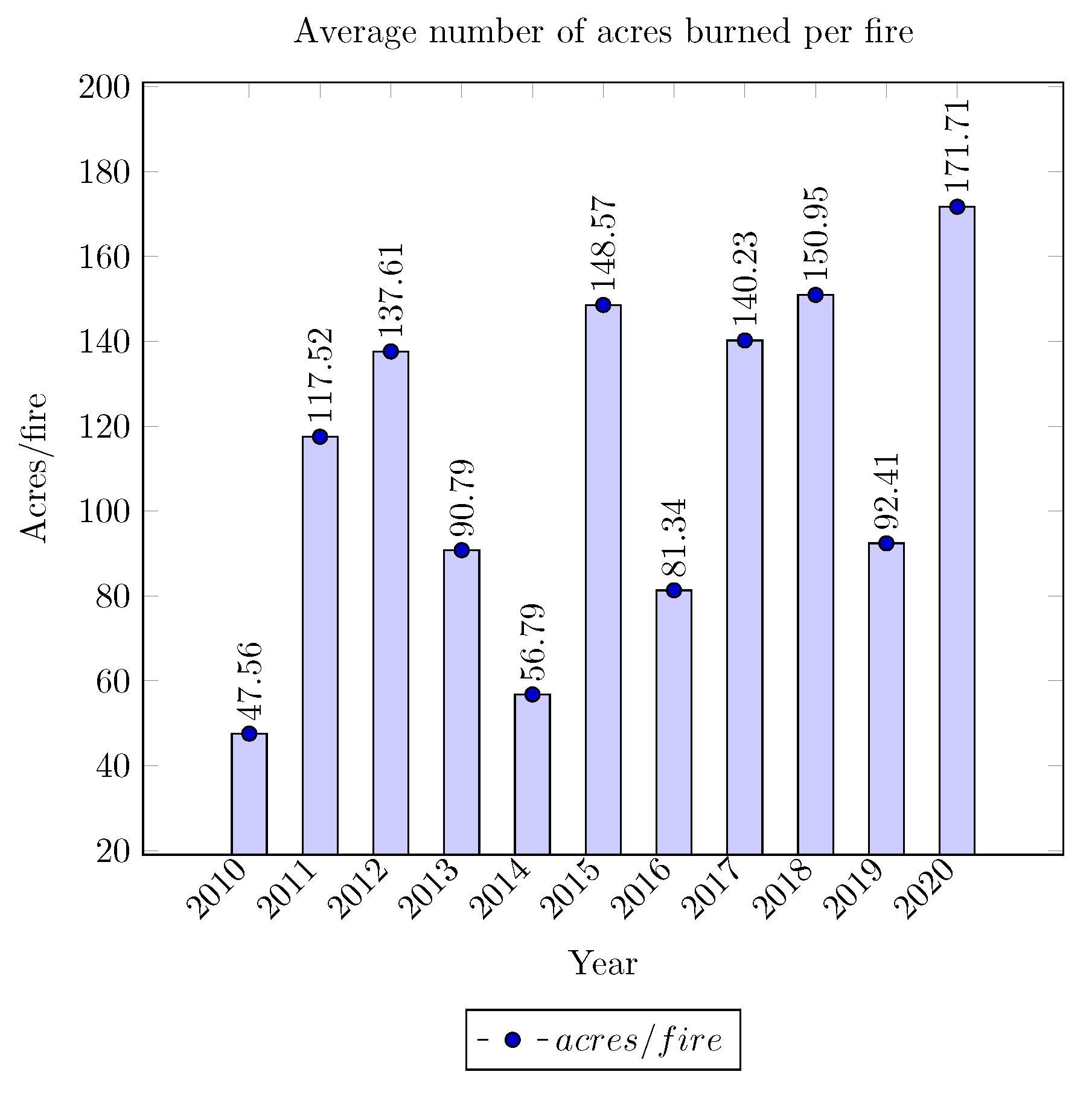
The average number of acres burned per wildfire data is presented in Figure 2. It is evident that there is an increase in the devastation caused by wildfires over the last decade. Similar trends can be observed in other places around the world. For example, in 2019, the number of wildfires in the Amazon rainforest increased by 80% compared to a year before. Approximately 75,000 wildfires were recorded just in 2019 in the Amazon rainforest. All data indicate that the development of accurate and reliable early wildfire detection systems is becoming a necessity.

Furthermore, there is also a growing awareness of the economic and social benefits associated with forests [4]. The methods for automatic wildfire detection, diagnosis, and prevention have been gaining more and more attention over the years. At the same time, remote sensing technologies and geographic information systems, as well as processes for data acquisition, are more accessible and versatile [5]. The main research challenges are associated with adequately analyzing and extracting knowledge from various sources of data. Continuous improvements in the field of artificial intelligence (AI), especially machine learning (ML), provide ample opportunities to design algorithms and methods to solve domain-specific problems, including the aforementioned problem of extracting knowledge from image data.

In recent years, computer vision-based wildfire prediction and detection systems have become very popular due to the rapid emergence and growth of technologies capable of analyzing large amounts of digital images with different artificial intelligence methods. Machine learning and deep learning (DL) methods are being increasingly applied to wildfire prediction and detection [6,7,8,9]. Unmanned aerial vehicles (UAVs) equipped with modern computer vision-based systems have great potential for detecting, monitoring, and fighting wildfires. A system for the automatic detection of wildfires is recommended for any wildlife preservation and protection organization, forestry management group, wildfire research organization, and other government or non-government agency.

In this paper, we propose a new method for the automated classification of wildfire images based on a modern deep learning approach for image classification. The proposed method is evaluated on two publicly available image datasets. In addition, a novel technique is presented for the efficient training of a lightweight CNN model in instances when the training data is scarce.

In this paper, a number of important contributions are made:

• A new dataset transformation method is proposed. This method increases the number of dataset samples and improves the training and generalization of the deep learning model. In instances when samples associated with one class are more prevalent than samples associated with other class(es), the proposed image dataset transformation method is able to improve the balance of the dataset;
• A new method for automatic classification of wildfire images based on a modern deep learning approach for image classification is presented. We propose a new lightweight deep convolutional neural network (CNN) model for the binary classification of wildfire images. In this paper, a certain number of lightweight configurations are considered. The results of prior empirical research, where many more configurations have been considered, indicate that the configurations that are presented in this paper offer higher performance with respect to the accuracy, execution time, and memory usage of the model. The model was tested on an additional dataset to show its capacity to generalize beyond the data it was trained on. Additionally, we extend our solution to work on multiclass classification;
• A best-performing model is identified as RT-LW-FIRE${100}_{12}$. It exhibits a range of favorable characteristics. The model is simple and can be rapidly and efficiently trained. It is capable of predicting an arbitrary image in 32 ms, which is approximately 31 frames per second (FPS); thus, it is suitable for real-time classification of wildfire images. The model is compact and can be implemented on less demanding hardware and deployed on a lightweight UAV platform. It exhibits high accuracy on the testing subset. One of the main motivations for this work is to create a model that can be implemented on a drone to efficiently detect, monitor, and fight against situations related to wildfire outbreaks.

The remainder of this article is organized as follows. Section 2 surveys the latest developments in the wildfire classification and detection that were gathered and distilled from the literature survey. Section 3 details a new method for wildfire classification with a deep convolution neural network. In Section 4, experimental results and evaluation criteria are presented. In Section 5, a discussion and comparison of results with state-of-the-art are presented. Finally, in Section 6, some conclusions are provided.

2. Related Work

Numerous fire detection methods and algorithms have been proposed in the recent literature. In this section, we review some works related to wildfire full-frame classification.

Dunnings et al. in [6], used simplified and experimentally optimized AlexNet and InceptionV1 CNN architectures for a frame-based binary fire detection task. For each architecture, different network configurations were experimentally assessed. For the AlexNet architecture, the authors considered 6 variations by removing a combination of 1–3 different CNN layers, while for InceptionV1, the authors considered 8 variations by removing up to 8 inception modules from the original architecture. The reported results showed that the reduction in model complexity, which also resulted in a reduction in the number of parameters (in millions), improved the classification accuracy. The authors have identified the best-performing model for AlexNet and InceptionV1. The model based on AlexNet was named FireNet, while the model based on InceptionV1 was named InceptionV1-OnFire. The accuracies of the optimized models were compared against the original AlexNet, InceptionV1, and VGG-13 models. The reported results indicated that it is possible to achieve 93% accuracy with InceptionV1-OnFire for the binary classification of fire images with 8.4 fps. The dataset used in this work is a collection of data from Chenebert et al. [10] (75,683 images), Steffens et al. [11] (20,593 images), also known as “furg-fire-dataset” [12], and material from public video sources (youtube.com: 269,426 images). The authors extracted 23,408 images from this collection to create a training subset, and 2931 images to create a testing subset.

Samarth et al. in [7], further explored this approach, i.e., the reduction in the complexity of the CNN model, and they have based their research on new architectures such as Inception, ResNet, and EfficientNet, and their combinations. They explored two detection problems: binary fire detection to detect the presence of fire in a frame and localization to detect the precise location of the fire within the frame. The authors explored InceptionV2, InceptionV3, InceptionV4, ResNet, a hybrid Inception-ResNet which is a combination between Inception and ResNet architectures, and EfficientNet. The authors identified the best variations, which they named as InceptionV3-OnFire and InceptionV4-OnFire. For the full-frame binary fire detection, these methods achieved 94.4% accuracy with InceptionV3-OnFire, and 95.6% accuracy with InceptionV4-OnFire, with 13.8 fps, and 12 fps, respectively.

In [8], Thomson et al. explored two CNN architectures to improve classification performance for real-time fire detection, which was based on experiments on NasNet-A-Mobile [13] and ShuffleNetV2 architectures [14]. Architectures were chosen because of their compactness and ability to provide high performance on ImageNet classification. The authors used transfer learning technique, whereby some layers within the original network are frozen, some layers are removed, and new layers to be trained on new data for fire classification are added. To be more precise, they removed only the last fully connected layer and added a new linear layer for binary classification. For the first half of training time, the entire architecture was frozen except the final linear layer, whilst for the remaining half of training time, the final convolutional layer in ShuffleNetV2 was unfrozen, and the final two reductions, normal cell iterations for NasNet-A-Mobile, were also unfrozen. The dataset used for training is the same dataset used in [6]. The best models were named NasNet-A-OnFire and ShuffleNetV2-OnFire with respect to the original models. The results indicated comparable performance to the models presented in [7], where NasNet-A-OnFire achieved 95.3% accuracy with 7 fps, and ShuffleNetV2-OnFire achieved 95% accuracy with 40 fps.

Sousaa et al. [9] proposed a transfer learning technique to optimize the InceptionV3 model that was pre-trained on the ImageNet dataset (1000 classes). InceptionV3 is a convolutional neural network with 48 layers in total. Different types of layers are used in the model: convolutional, two types of pooling layers (max and average), fully connected, dropout, and a softmax classifier. A dataset called the cross-validation database (CVDB) was created as a subset from the Portuguese Firefighters Portal Database (PFPDB), which was created from 3900 images and images from the data augmentation. Data augmentation was used to generate more training samples and reduce overfitting. A total of 3623 fire and 3551 not fire images were used. The dataset was partitioned with k-fold cross-validation, where k = 10. The model resulted in 93.6% ± 1.57 accuracy.

Jadon et al. in [15], presented FireNet as a lightweight shallow neural network that could be employed on embedded platforms such as Raspberry Pi. The network was built from scratch and trained on a dataset that was also presented in the paper. The dataset consists of 46 fire videos (19,094 images) with 16 non-fire videos (6747 images), and an additional 160 non-fire images [16]. The model achieved 93.91% accuracy.

3. Materials and Methods

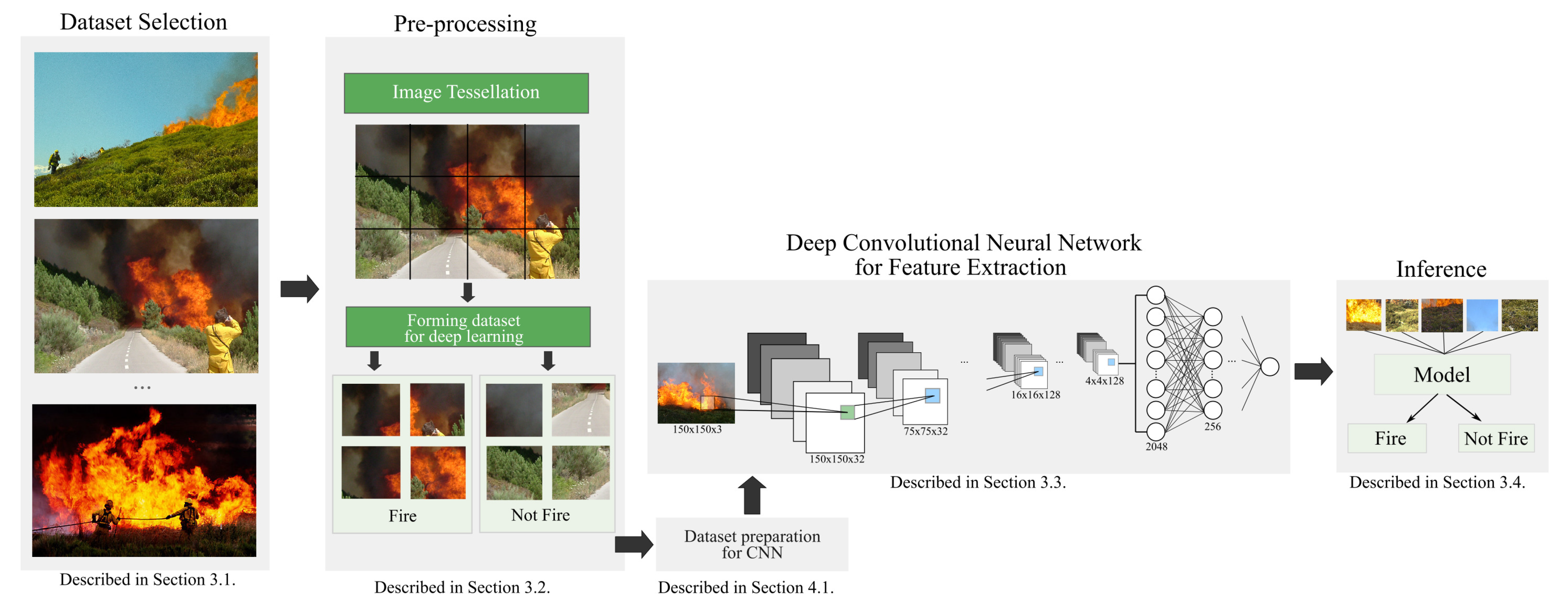
The overall design of our method is illustrated in Figure 3. We first describe the process of dataset selection. Then, we present the three major phases in the following subsections: pre-processing, a lightweight CNN for wildfire image classification, and inference.

3.1. Dataset Selection

From the literature review, we observed that existing datasets are mostly created from video data of fire and non-fire scenarios. The problem with this approach is that these images are very similar; the background is the same in the frames of one video, hence, the change between frames is minimal. Video sources might not be suitable for a robust and versatile deep learning model because frames are very similar, especially if the model is planned to be used in real-life wildfire scenarios.

In this work, we use the Corsican Fire DataBase (CFDB) [17,18]. This is an open image database that contains 500 visual range fire images. Image acquisitions were based on different camera positioning, vision, weather, vegetation, distance from the fire, and brightness. Every image in the dataset is characterized by 22 parameters, i.e., camera model, sensitivity, exposure time, GPS position, the direction of propagation of the fire, the color of the smoke, presence of clouds, etc. All images have been associated with the corresponding ground truth images.

In the context of the development of deep learning models and applications, this dataset is challenging, as it only contains 500 images. However, images contain real-life scenarios of wildfire images, and as such, the authors believe they can facilitate the development of a model to be applied in real-life applications. A few examples of images from this dataset are shown in Figure 3. In this paper, we show that it is possible to use the CFDB dataset to train a deep learning model.

3.2. Pre-Processing

In this subsection, we address the problem of having a dataset of images with a relatively small number of images. We begin by acknowledging the fact that, in order to increase the capacity of a machine learning model to generalize beyond the training data, the training dataset should have a sufficient number of statistically relevant samples.

One of the most popular techniques for increasing the size of the labeled training sets is data augmentation. In this technique, the training data is increased by applying various class-preserving transformations. This means that all subsequently augmented sub-images inherit the same label as the original image. This is contrary to the idea presented in this paper. The motivation for our method comes from the fact that the vast majority of CNN models resize the original image to a tensor of a specific dimension defined by a neural model, which results in the loss of valuable data. We observe that the data can be used more efficiently by representing smaller parts of the image as the input data to the model. In this process, it is important to differentiate between the data with different information, e.g., “there is a fire on the image” or “there is no fire on the image”. Hence, we design a strategy that pre-processes data and then use it to obtain maximal data usage in the training process.

Since the chosen dataset contains a small number of images with favorable characteristics, in this subsection, we propose a method to increase the number of dataset samples. The proposed method can also be used to address the problem of having an imbalanced dataset, whereby images associated with one class are more frequent than the images associated with other class(es). In this paper, the proposed method for image dataset transformation is used to improve the training and generalization of the proposed model for wildfire image classifications.

The CFDB dataset contains $T=500$ images. Images are not presented with uniform resolution. The resolution of images ranges from $183\times 242$ to $4000\times 3000$, while the number of pixels ranges from a minimum of 44.3 k to a maximum of 12 M pixels. Some images contain large fire regions; however, the majority of the images contain only some small fire regions. In real-life situations, it is important to detect early signs of fire, so increasing the chance of detection of early signs of fire, which might be presented by a small region of fire in an image, is very important. Since this dataset represents important data captured in real-life scenarios, we use this dataset to create a new dataset by applying a tessellation method that is performed on original images. This results in creating many smaller images that are denoted as sub-images. Sub-images are used to increase the detection accuracy of a deep learning model, hence providing a greater possibility for the detection of wildfire in real-life scenarios.

In this phase, the images are prepared for the training process of a new lightweight CNN for wildfire image classification described in Section 3.3. The major pre-processing steps can be grouped into two stages: (1) image tessellation, and (2) formation of a dataset for deep learning.

3.2.1. Image Tessellation

The principal idea behind this algorithm is to mitigate the problem of information loss due to a common practice of deep learning models to resize an input image to a tensor of a specific dimension. A dimension is usually defined by a neural model that is being used. For example, VGG, InceptionNet, ResNet, and many other models resize an image into a 224 × 224 × 3 tensor before the training and testing process begins. Resizing an image implies changing its dimension, which can be accomplished by changing only the width or the height, or both at the same time. The preferred method for resizing is resampling using pixel area relation. If a dataset consists of images of different resolutions, this means that all images will be resized into 224 × 224 × 3. This inevitably leads to information loss, and it was one of our motivations for our work. To prevent unnecessary information loss, we propose a new method based on an image tessellation scheme to produce sub-images of comparable sizes. This method will also increase the number of dataset samples. To the best of our knowledge, this is the first time that this method was used for training a deep learning network.

Every image I in the dataset is divided into an even number of sub-images, denoted as N. The total number of sub-images, $T_N$, depends only on a selected number N. It is independent of the image size. Image I is divided into $X\times Y$ sub-images, where X and Y are chosen to preserve the approximate proportion of each sub-image. Since N is an even number, at least one number, X or Y, has to be an even number. Two image tessellation scenarios are considered in this paper, as shown in

Table 1. Two values of N divide an image from the CFDB dataset into different set of tiles, which results in different numbers of sub-images per N.

N	Tiles ($\mathit{X}\times \mathit{Y}$)	No. Sub-Images (${\mathit{T}}_{\mathit{N}}$)
12	$4\times 3$	6000
42	$7\times 6$	21,000

. Other scenarios are possible, but the CNN models developed under the considered scenarios exhibit satisfactory accuracy. In the first sub-stage, every image I from the dataset is divided into an even number of sub-images N.

When $N=12$, the image width is divided by $X=4$, and the height is divided by $Y=3$. When $N=42$, the image width is divided by $X=7$, and the height is divided by $Y=6$. If $N=10$ or $N=40$, the image tessellation tool can result in sub-image sizes that are disproportional, e.g., $5\times 2$ or $8\times 5$, which should generally be avoided because images are resized before training, so data loss might occur. A better tessellation scheme can be attained with $N=42$, which results in $7\times 6$ tiles. It is important to carefully choose an adequate number of sub-images so that the aspect ratio of the resulting sub-images is similar to the original image.

Irrespective of image resolution, the total number of sub-images derived from a given image is completely defined by the value assigned to the parameter N. If there are $T=500$ images in the dataset, then the total number of sub-images is calculated as $T_N=T\times N$. For different tessellation scenarios, the total number of sub-images is provided in Table 1. It is evident that for a relatively small number of N, a substantial number of dataset samples is generated. These sub-images (dataset samples) may or may not contain pixels associated with fire.

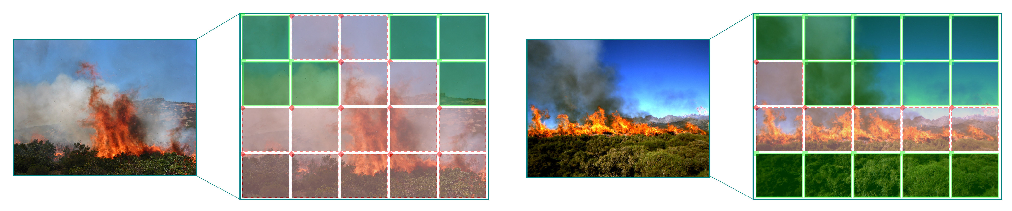
Two examples of images and the results of an image tessellation scheme based on $N=20$ are presented in Figure 4, where sub-images containing fire are shown with a red overlay. For example, a $4000\times 3000$ image is tessellated into 20 sub-images with a resolution of $800\times 750$. A sub-image of this size is considered suitable to be used in the process of training a deep learning model. Once the results of the selected image tessellation scheme are obtained, it is necessary to assign a label (fire or not fire) to all individual sub-images.

3.2.2. Formation of a Dataset for Deep Learning

Manual classification of sub-images into two classes, fire and not fire, is a labor-intensive and time-consuming task. It cannot be accomplished without professional knowledge and extensive experience in the field. Additionally, this approach does not scale very well for different tessellation strategies and large-scale datasets.

Labeling of sub-images is necessary to facilitate supervised learning. The process can be automated if the dataset is associated with ground truth images, or when an unsupervised method exists for the image classification. The CFDB dataset has associated ground truth images. Thus, we performed the same tessellation process on the ground truth images as on the original images, as was described in Section 3.2.1. The F1 score was calculated for each sub-image. We used an existing unsupervised method [19] to classify sub-images into two classes (fire and not-fire) based on the F1 score. We adapted this method to account for the specificities associated with the problem currently being addressed. Images that have a high F1 score are declared to belong to the “fire” class, while the rest belong to the “not-fire” class. In special cases, such as when a sub-image contains a very small number of fire pixels, we declare a sub-image to belong to the “not fire” class. This situation usually occurs on the edges of a sub-image that typically represents a small amount of smoke.

At the end of this step, a new dataset with only two classes is created. Additional steps are required to prepare the dataset for deep learning as is described in Section 4.1.

3.3. LW-FIRE: A Lightweight CNN for Wildfire Image Classification

In recent years, deep learning has demonstrated very promising results in a range of different engineering applications. DL-based models have the ability to automatically learn features from various data sources, and it has more robustness than other ML-based methods. Over the years, various DL-based models and applications have been developed [20,21,22,23,24]. However, one of the downsides of DL methods is an extensive training phase, which usually requires a large training dataset to attain the required functionality. More data always mean more training time and more computational resources—typically high-end GPUs or CPUs. Due to memory constraints, a model with a large number of learnable parameters and arithmetic operations is computationally expensive and can be trained for days to attain reasonable accuracy [25].

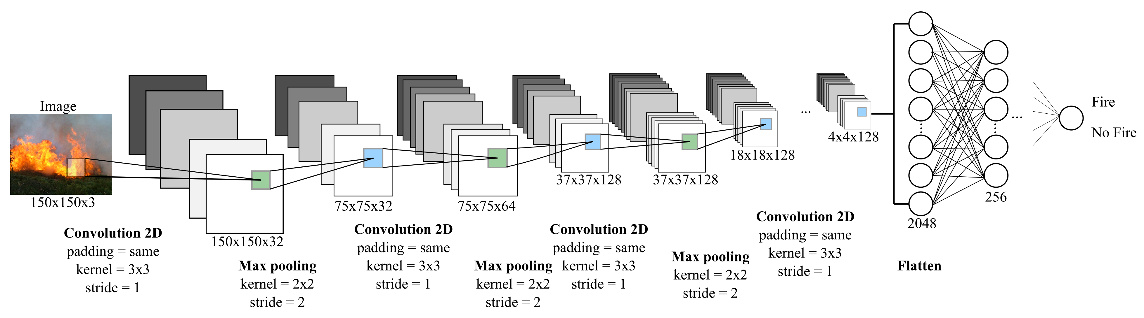
In this paper, we propose a new lightweight wildfire CNN for image classification. The CNN model can be trained in a reasonable time and computational resources (CPUs or GPUs, and memory), and is also suitable for real-time fire detection applications. LW-FIRE is an abbreviation for the Lightweight WildFIRE classification model. When a model has the real-time performance we add the “RT” prefix to the name of a model. The architecture of the basic Lightweight CNN for wildfire image classification is illustrated in Figure 5. The specification of layers and number of parameters is provided in

Table 2. Summary of the LW-FIRE150 deep convolutional neural network architecture.

No.	Block Type	Block Description	Size of Feature Maps	No. Parameters
1	Conv2D (ReLU)	2D convolution layer	(150, 150, 32)	896
2	BatchNormalization	Batch normalization layer	(75, 75, 32)	128
3	MaxPooling2D	Max pooling for 2D data	(75, 75, 32)	0
4	Conv2D (ReLU)	2D convolution layer	(75, 75, 64)	18,496
5	BatchNormalization	Batch normalization layer	(75, 75, 64)	256
6	MaxPooling2D	Max pooling for 2D data	(37, 37, 64)	0
7	Conv2D (ReLU)	2D convolution layer	(37, 37, 128)	73,856
8	BatchNormalization	Batch normalization layer	(37, 37, 128)	512
9	MaxPooling2D	Max pooling for 2D data	(18, 18, 128)	0
10	Conv2D (ReLU)	2D convolution layer	(18, 18, 128)	147,584
11	BatchNormalization	Batch normalization layer	(18, 18, 128)	512
12	MaxPooling2D	Max pooling for 2D data	(9, 9, 128)	0
13	Conv2D (ReLU)	2D convolution layer	(9, 9, 128)	147,584
14	BatchNormalization	Batch normalization layer	(9, 9, 128)	512
15	Conv2D (ReLU)	2D convolution layer	(9, 9, 128)	147,584
16	BatchNormalization	Batch normalization layer	(9, 9, 128)	512
17	MaxPooling2D	Max pooling for 2D data	(4, 4, 128)	0
18	Flatten	Flattens the input	2048	0
19	Dense (ReLU)	Densely connected NN layer	256	524,544
20	Dropout	Dropout regularization with rate 0.6	256	0
21	Dense (ReLU)	Densely connected NN layer	128	32,896
22	Dropout	Dropout regularization with rate 0.3	128	0
23	Dense (ReLU)	Densely connected NN layer	64	8256
24	Dropout	Dropout regularization with rate 0.15	64	0
25	Dense (ReLU)	Densely connected NN layer	32	2080
26	Dropout	Dropout regularization with rate 0.075	32	0
27	Dense (ReLU)	Densely connected NN layer	16	528
28	Dropout	Dropout regularization with rate 0.0325	16	0
29	Dense (Sigmoid)	Densely connected NN layer	1	17
			Total No. parameters:	1,106,753

. The structure of the CNN model was created with an extensive experimentation process and commonly observed practices from the DL community. From the experiments, we observed some favorable characteristics of the model on the validation dataset. Once the model achieved satisfied accuracy on the validation set, we tested our models on the three different testing sets. The process of evaluation is described in Section 5.

The input layer uses a set of 3-channel input images. The total number of images depends on the sub-image configuration chosen in the previous stage. We considered two configurations, as shown in Table 1: (i) N = 12 and (ii) N = 42, where the number of images $T_N=6000$ and $T_N$ = 21,000, respectively. The first convolution layer uses 32 output filters ($3\times 3$) followed by batch normalization and a max-pooling layer with $2\times 2$ strides. The second convolution layer uses 64 output filters followed by batch normalization and max-pooling layer. Then, an additional convolution layer with 128 output filters is followed by batch normalization and max-pooling layers. Outputs from the last max-pooling layer are flattened and connected with several fully connected (FC or Dense) layers, where ReLU and Sigmoid activation functions are used, respectively. Non-linearity is introduced in all convolution layers with the ReLU activation function. The ReLU activation function significantly reduces the time for model convergence. The max-pooling layer is used after the convolution layers to reduce the spatial dimensionality of the output feature maps.

A batch normalization (BN) layer was added after every convolution layer to normalize the values in the batch of images and to encourage stable estimation. This technique reduces the overfitting problem [26]. Finally, we introduced several dense layers with dropout regularization techniques that randomly set hidden units to 0 with different frequency ratings. The dropout layer is applied only during the training stage.

3.4. Inference

After a DL-based model is trained and validated with the training and validation subsets to perform binary classification, its performance is evaluated on the test subset. The data split strategy is described in Section 4.1. The performance of the model is evaluated in terms of various measures based on the confusion matrix and processing speed defined in terms of average frames per second. Every test yields a prediction (“fire” or “not fire”) and the time required for the prediction. We use this information to generate the testing accuracy of the model, execution time, and average frames per second.

4. Results

4.1. Evaluation Criteria

The transformed dataset consists of original images and sub-images, created in the pre-processing phase. The samples are split into three subsets: training, validation, and testing. We first randomly shuffled image data, and then divided them into 70% samples for training, 10% for validation, and 20% for testing. We trained our model on the training set and fine-tuned the hyperparameters on the validation set. The evaluation of the performance of the model was carried out on the testing subset.

Table 3. Number of images in each sub-set of dataset used for training, validation and testing.

N	Training Set (Fire, Not Fire)	Validation Set (Fire, Not Fire)	Test Set (Fire, Not Fire)
12	4552	652	1297
	(2735; 1817)	(394; 258)	(779; 518)
42	15,050	2149	4304
	(6208; 8842)	(910; 1239)	(1774; 2530)

provides more details about the number of samples used in each subset.

The predictive ability of the models is evaluated using the evaluation criteria based on the confusion matrix (contingency table), with four different results: true positives (TP), true negatives (TN), false positives (FP), and false negatives (FN). Evaluation criteria used for the model performance are the sensitivity or true positive rate (TPR), specificity or true negative rate (TNR), fall-out or false positive rate (FPR), precision or positive predictive value (PPV), accuracy (ACC), F1 Score, Matthews correlation coefficient (MCC), and Fowlkes—Mallows index (FM), as is defined in Equations (1)–(8).

$$\mathrm{TPR}=\frac{\mathrm{TP}}{\mathrm{TP}+\mathrm{FN}}$$

(1)

$$\mathrm{FPR}=\frac{\mathrm{FP}}{\mathrm{FP}+\mathrm{TN}}=1-\mathrm{TNR}$$

(2)

$$\mathrm{TNR}=\frac{\mathrm{TN}}{\mathrm{TN}+\mathrm{TP}}$$

(3)

$$\mathrm{PPV}=\frac{\mathrm{TP}}{\mathrm{TP}+\mathrm{FP}}$$

(4)

$$\mathrm{ACC}=\frac{\mathrm{TP}+\mathrm{TN}}{\mathrm{TP}+\mathrm{TN}+\mathrm{FP}+\mathrm{FN}}$$

(5)

$${\mathrm{F}}_1=\frac{2·\mathrm{TP}}{2·\mathrm{TP}+\mathrm{FP}+\mathrm{FN}}$$

(6)

$$\mathrm{MCC}=\frac{\mathrm{TP}\times \mathrm{TN}-\mathrm{FP}\times \mathrm{FN}}{\sqrt{(\mathrm{TP}+\mathrm{FP}\left)\right(\mathrm{TP}+\mathrm{FN}\left)\right(\mathrm{TN}+\mathrm{FP}\left)\right(\mathrm{TN}+\mathrm{FN})}}$$

(7)

$$\mathrm{FM}=\sqrt{\frac{\mathrm{TP}}{\mathrm{TP}+\mathrm{FP}}\times \frac{\mathrm{TP}}{\mathrm{TP}+\mathrm{FN}}}=\sqrt{\mathrm{PPV}\times \mathrm{TPR}}$$

(8)

4.2. Experimental Setup

The model was designed with Keras with a TensorFlow backend and was trained and tested on an Intel Core i7-10700KF CPU @ 3.80GHz with 32GB memory.

An adaptive learning rate optimizer (Adam) was used as an optimization algorithm to adjust the weights of the CNN model. Adam is used for first-order gradient-based optimization of the stochastic objective function, which is based on adaptive estimates of lower-order moments [27]. We used a mini-batch training scheme for feeding image data into the proposed model. This scheme ensures that we trained the model with a balanced training set during the training epochs. Parameters used with the optimizer are the learning rate $\alpha =0.001$, the exponential decay rates for the first and second-moment estimates ${\beta }_1=0.9$ and ${\beta }_2=0.999$, and a very small number to prevent any division by zero $ϵ=1\times {10}^{-8}$. The batch size is set to 32 for training and validation.

4.3. Classification Performance of the Proposed Framework

We consider two parameters when defining a model:

1.

The type of image tessellation scheme, as defined in Table 3, and

2.

The sample resolution R used for training, validation and testing, where R = 100, 150, 300, and possible resolutions are defined as $100\times 100$, $150\times 150$, and $300\times 300$.

Based on different combinations of two different image tessellation schemes and sample (sub-image) resolution, six different models are developed, as is shown in

Table 4. Six proposed models based on different image tessellation schemes and three different sub-image resolutions.

No.	Model	Number of Tiles/Image	Resolution
1	RT-LW-FIRE100${}_{12}$	$N=12$	$100\times 100$
2	LW-FIRE150${}_{12}$	$N=12$	$150\times 150$
3	LW-FIRE300${}_{12}$	$N=12$	$300\times 300$
4	LW-FIRE100${}_{42}$	$N=42$	$100\times 100$
5	LW-FIRE150${}_{42}$	$N=42$	$150\times 150$
6	LW-FIRE300${}_{42}$	$N=42$	$300\times 300$

. In accordance with the associated image tessellation scheme, the performance of each model is presented in

Table 5. Different configurations and their performance measures for $N=12$ and $N=42$.

Model	Image	No. Parameters	Epochs	Validation Accuracy	Testing Accuracy	FPS
RT-LW-FIRE100${}_{12}$	$100\times 100$	877,377	27/50	97.8%	96.1%	31.25 fps
LW-FIRE150${}_{12}$	$150\times 150$	1,106,753	29/50	98.13%	95.83%	27.7 fps
LW-FIRE300${}_{12}$	$300\times 300$	3,236,673	18/50	97.5%	95.4%	19.6 fps
LW-FIRE100${}_{42}$	$100\times 100$	877,377	32/50	98.44%	97.1%	27 fps
LW-FIRE150${}_{42}$	$150\times 150$	1,106,753	35/50	99.36%	97.25%	25.6 fps
LW-FIRE300${}_{42}$	$300\times 300$	3,236,673	6/50	98.13%	96.4%	20 fps

.

The performance of each model is presented in Table 5. The resolution R determines the total number of parameters. The models reach optimal performance in different epochs, as denoted in the column “Epochs”. The maximum number of epochs used in all tests is 50. More epochs were used in the experimental phase, but no significant improvement in terms of accuracy was observed; thus, we limited the number of epochs to 50. The validation accuracy in Table 5 is the accuracy of the optimal model with respect to the specific epoch displayed in the column “Epochs”. The average frames per second are calculated with respect to the number of images from the test set (Table 3).

The RT-LW-FIRE100${}_{12}$ model has 877,377 parameters and requires approximately 50 min to train. Its validation accuracy is 97.8%, and the testing accuracy is 96.1%. The model can make a prediction in 32 ms, and this enables processing of 31.25 FPS. In literature, the requirement for real-time capabilities is typically set to 30 fps, as is discussed in [28,29,30]. This sets the limitation for image processing time to at least 33.3 ms. The reason for providing the real-time capabilities is to enable the implementation of our method on embedded devices, such as the ones used in drones. In return, this will help in alarming the firefighting forces immediately after the wildfire is detected.

The highest validation accuracy of the RT-LW-FIRE100${}_{12}$ model is reached in 27 epochs. The other two models based on the same image tessellation scheme are denoted as LW-FIRE${150}_{12}$ and LWFIRE${300}_{12}$. These models reached the optimal validation accuracy after the 29th and 18th epochs, respectively.

The number of parameters increases with increasing image resolution. Even though more data is analyzed, results do not indicate a significant increase in performance, as is shown in the “Testing accuracy” column. However, the number of parameters causes the number of floating-point operations to increase. Hence, FPS is significantly decreased. Models also need more time to be trained, which is especially noticeable in the last configuration, where training can last up to seven hours.

The LW-FIRE100${}_{42}$ model has the same number of parameters as the RT-LW-FIRE100${}_{42}$. Its validation accuracy is 98.44%, and its testing accuracy is 97.1%. On the test dataset, it can make a prediction in 37 ms, which is approximately 27 fps. This model is very close to reaching real-time capabilities. With better hardware or sophisticated optimizations (such as Intel’s OpenVINO), this model could potentially be used in real-time applications. The best validation accuracy is reached after 32 epochs.

The next model, LW-FIRE150${}_{42}$, has 1,106,753 parameters. The best validation accuracy is reached after the 35th epochs of training and it is 99.36%, while the testing accuracy is 97.25%. An image is processed in 39 ms, which implies that the model can predict 25.6 images (frames) per second. In terms of the performance on the test dataset, this model is the best model of all models that share this image tessellation scheme.

The model LW-FIRE300${}_{42}$ has 3,236,673 parameters. The training time increased because the amount of data in the training phase also increased. The best validation accuracy is reached after the 6th epoch, and it is 98.1%, while the testing accuracy is 96.4%. On average, a test image is processed in 51 ms, which indicates a processing speed of 19.6 frames per second.

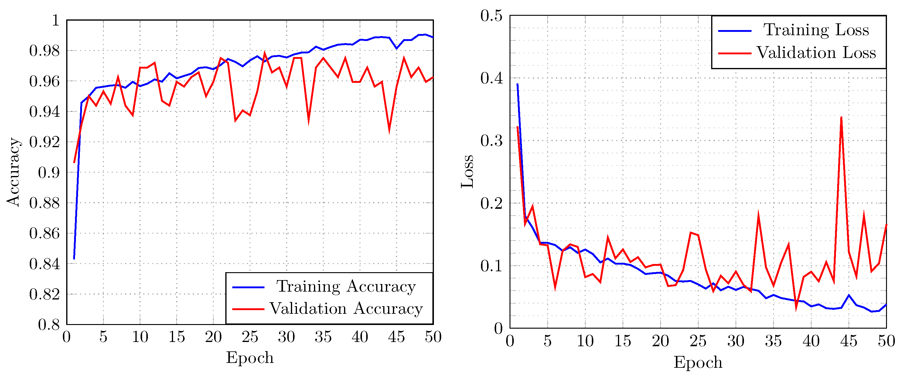
In Figure 6, we present the overall performance of the best performing model (LW-FIRE150${}_{42}$) in terms of accuracy on the testing subset. The model displays stability and robustness. It also shows that adding the batch normalization and dropout layers prevented overfitting.

4.4. Multiclass Classification

In this paper, we addressed the problem of wildfire image classification. We described a new deep learning-based model, and the dataset transformation on the example of two classes, namely “fire” and “not fire”. In this subsection, we provide sufficient evidence that our solution can be extended to work on multiclass classification.

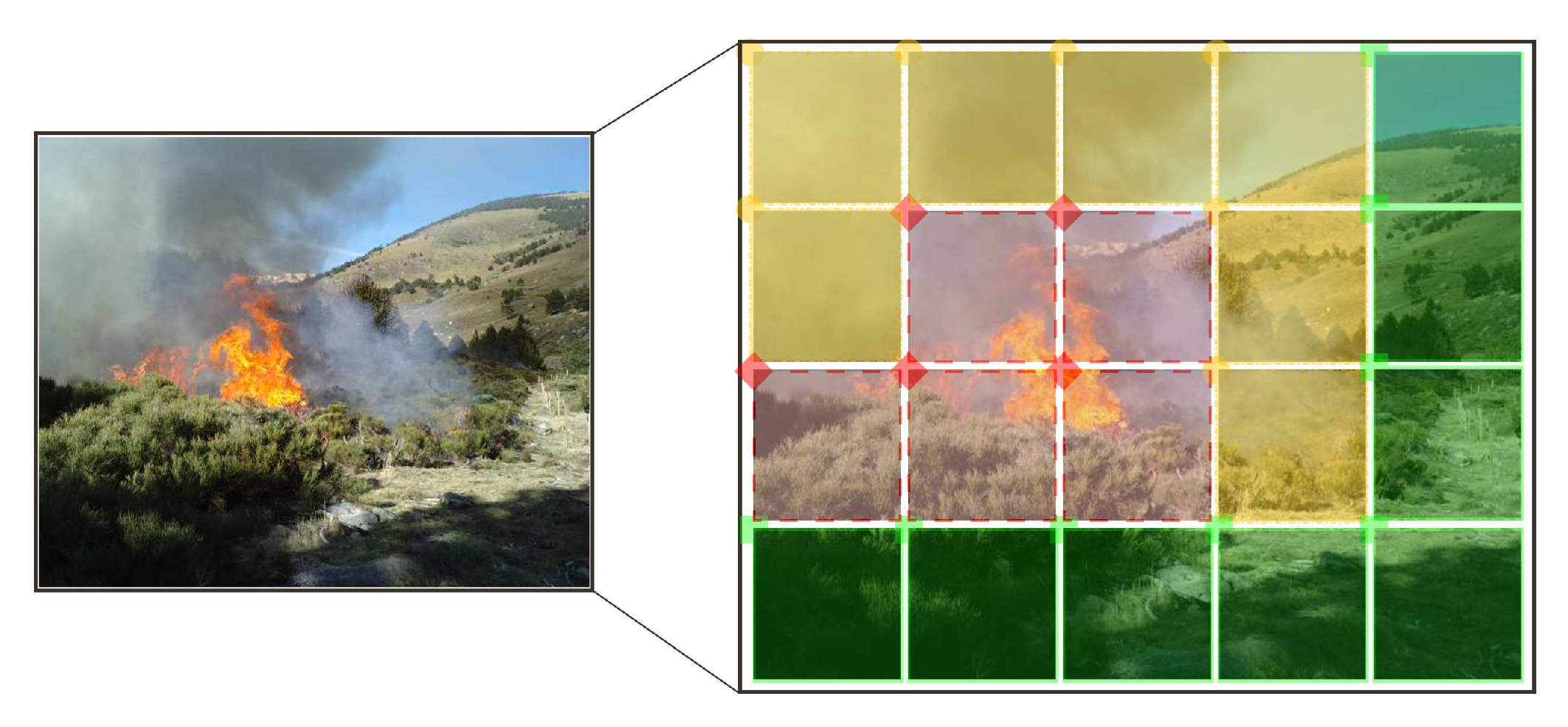
The number of possible classes is typically related to a specific application domain. Since we addressed the classification of wildfire images, we believe that the extension of this problem to include the class “smoke” is a logical choice. To prepare the dataset for multiclass classification, we use the same image tessellation technique described in Section 3.2.1, but now we also define a third class: “smoke”. The sub-images created in the image tessellation step need to be labeled with appropriate labels. Sub-images that are labeled as “fire” in the binary classification problem can still be used. On the other hand, sub-images that are labeled as “not fire” can contain information that is associated with smoke or not smoke or fire. Thus, we manually selected sub-images associated with smoke from the “not fire” class, and labeled them as “smoke”. The rest of the images remained with the label “not fire”. In Figure 7, we provide a visual representation of how an image can be divided into three classes. Next, the labels are encoded as categorical vectors. The same technique that is described here can be applied to other application domains. Once the dataset is prepared, the CNN model needs to be modified to support the multiclass classification.

Multiclass classification is demonstrated with the LW-FIRE${150}_{42}$ model. The model is modified to generate three output signals instead of the one which is used for binary classification. During the training, the categorical cross-entropy function is used as a loss function. The same strategy is used to divide the samples, i.e., 70% of samples were used for training, 10% for validation, and 20% for testing. The model was trained for 50 epochs. The best validation accuracy was obtained after the 39th epoch, and the accuracy was 95.3%. After testing our model on a testing subset, we noticed that the overall accuracy increased to 98.6%. This is because the sub-images from the “not fire” class are divided into two classes, which increased the differentiation between the “not fire” and “smoke” classes, and, subsequently, the “fire” class. Hence, the model identified sub-images with fire more easily. Analysis of results revealed the increase in true positives and the decrease in false negatives, which had a positive effect on the majority of metrics used in this paper.

5. Discussion

In this section, we provide a comparison between the six state-of-the-art models discussed in Section 2 and the best models proposed in this work. We measured the performance of all models on the same hardware configuration and provide the results of eight metrics described in Section 4.1. We evaluated the following models:

1.

FireNet [6];

2.

InceptionNetV1-OnFire [6];

3.

InceptionNetV3-OnFire [7];

4.

InceptionNetV4-OnFire [7];

5.

NasNet-A-OnFire [8];

6.

ShuffleNetV2-OnFire [8];

7.

Our LW-FIRE100${}_{12}$ model, and;

8.

Our LW-FIRE150${}_{42}$ model.

Models 1–6 were trained on the dataset presented in [6]. The dataset was created by combining several other datasets, i.e., data from Chenebert et al. [10] (75,683 images), Steffens et al. [11] (20,593 images), also known as the “furg-fire-dataset” [12], and material from public video sources (youtube.com: 269,426 images). The authors then extracted 23,408 images from this collection to create a new dataset for training (12,550 images of fire, and 10,858 images of not-fire). The testing subset consists of 2931 images.

Models 7–8 were trained on the transformed CFDB dataset, as described in Section 3. The generalization of two of our models was demonstrated not only on the testing subset of this dataset but also on a testing subset from [6]. Besides the model’s architecture, better generalization is achieved through the introduction of the dataset transformation technique, which increased the data usage from the dataset. To provide a fair comparison between the presented models, we performed two experiments:

1.

Experiment I: All models have been tested on the Dunnings dataset used in [6]. Results are presented in

Table 6. Comparison with the state of the art on the dataset presented in [6]. Our model was not trained on this dataset, though other models have been trained and tested on this dataset. * Evaluated on $2\times 2$ tiles of images in this dataset (as presented in Figure 8).

#	Model	TPR	FPR	TNR	PPV	ACC	F1	MCC	FM
#1	FireNet [6]	0.846	0.0831	0.916	0.910	0.881	0.877	0.765	0.878
#2	InceptionNetV1-OnFire [6]	0.810	0.0666	0.933	0.924	0.871	0.863	0.749	0.865
#3	InceptionNetV3-OnFire [7]	0.949	0.078	0.9218	0.9239	0.9358	0.9367	0.872	0.936
#4	InceptionNetV4-OnFire [7]	0.9481	0.0477	0.952	0.952	0.950	0.950	0.900	0.950
#5	NasNet-A-OnFire [8]	0.973	0.082	0.917	0.922	0.945	0.947	0.892	0.947
#6	ShuffleNetV2-OnFire [8]	0.960	0.078	0.921	0.9247	0.941	0.942	0.883	0.942
#8	Our LW-FIRE150${}_{42}$ *	0.980	0.091	0.908	0.914	0.944	0.946	0.891	0.946

;

2.

Experiment II: All models have been testes on the dataset configurations created in this work based on the CFDB dataset. Results are presented in

Table 7. Comparison with the state of the art on the dataset presented in this paper ($N=12$).

#	Model	TPR	FPR	TNR	PPV	ACC	F1	MCC	FM
#1	FireNet [6]	0.727	0.0559	0.944	0.928	0.835	0.816	0.688	0.8226
#2	InceptionNetV1-OnFire [6]	0.708	0.055	0.944	0.926	0.826	0.803	0.671	0.810
#3	InceptionNetV3-OnFire [7]	0.794	0.028	0.971	0.964	0.882	0.871	0.777	0.875
#4	InceptionNetV4-OnFire [7]	0.869	0.036	0.963	0.959	0.916	0.912	0.836	0.913
#5	NasNet-A-OnFire [8]	0.820	0.0637	0.936	0.927	0.878	0.870	0.761	0.872
#6	ShuffleNetV2-OnFire [8]	0.820	0.025	0.974	0.970	0.897	0.889	0.804	0.892
#7	Our RT-LW-FIRE100${}_{12}$	0.966	0.063	0.936	0.938	0.951	0.952	0.903	0.952

and

Table 8. Comparison with the state of the art on the dataset presented in this paper ($N=42$).

#	Model	TPR	FPR	TNR	PPV	ACC	F1	MCC	FM
#1	FireNet [6]	0.695	0.039	0.960	0.946	0.827	0.801	0.679	0.810
#2	InceptionNetV1-OnFire [6]	0.598	0.020	0.979	0.966	0.788	0.738	0.624	0.760
#3	InceptionNetV3-OnFire [7]	0.769	0.030	0.969	0.961	0.869	0.854	0.753	0.860
#4	InceptionNetV4-OnFire [7]	0.753	0.0328	0.967	0.958	0.860	0.843	0.737	0.849
#5	NasNet-A-OnFire [8]	0.730	0.009	0.990	0.987	0.860	0.839	0.746	0.849
#6	ShuffleNetV2-OnFire [8]	0.791	0.013	0.986	0.983	0.889	0.877	0.793	0.882
#8	Our LW-FIRE150${}_{42}$	0.976	0.030	0.969	0.970	0.973	0.973	0.946	0.973

, for $N=12$ and $N=42$, respectively.

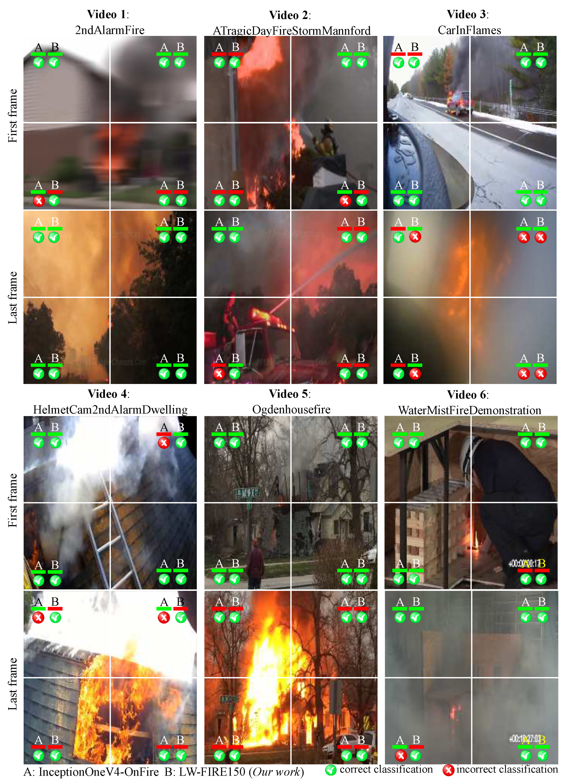
In Experiment I, we used a testing subset from [6], which consists of 2931 images extracted from six video sources. Some examples of images are provided in Figure 8, where we show the first and last frame of six video sources from the testing subset. In Table 6, we present the results. Models 1–6 have been evaluated on the original images, while our model LW-FIRE150${}_{42}$ was evaluated on $2\times 2$ sub-images. In this case, an image was considered to belong to the “fire” class if any of the sub-images has been classified as a “fire” image.

In Figure 8, we show the performance on $2\times 2$ sub-images of two models: InceptionOne V4-OnFire, which has the best overall performance on this dataset, and our LW-FIRE150${}_{42}$. The state-of-the-art models performed better on the original size images, while LW-FIRE150${}_{42}$ performed better on sub-images, as was expected. We evaluated our model on $2\times 2$ sub-images to show that our model can achieve a higher true positive rate (TPR) than the state-of-the-art models, while in other metrics, it shows comparable results. The results of our model could be improved if the false positive rate (FPR) is improved, which would have a positive effect on other metrics. Our model also outperformed FireNet, InceptionNetV1-OnFire, InceptionNetV3-OnFire, and ShuffleNetV2-OnFire when we consider metrics such as ACC, F1, MCC, and FM.

The classification accuracy is demonstrated in Figure 8. For example, InceptionOneV4-OnFire (A) could not classify one of the sub-images as fire in the first frame of Video 1 and 2, while the last frame of Video 2 misclassified a fire truck as a “fire”. In the first frame of Video 4, the model misclassified smoke as fire on one of the sub-images. In the last frame of Video 4, it failed to classify two sub-images as fire, and in Video 6, one sub-image as fire. In these examples, our model (B) correctly classified sub-images as “fire” or “not-fire” images. However, it misclassified sub-images in Video 3, where both algorithms have shown bad classification results. The results of the first frame of Video 3, 5, and 6, and the last frame of Video 1 and Video 5 show identical results of both models. On this statistical sample, LW-FIRE150${}_{42}$ performed better, and it showed better performance in the overall results in this experiment, which is also reflected in Table 6.

In Experiment II, we tested all models on the dataset described in this paper, where $N=12$ and $N=42$. The testing subset for $N=12$ has 1297 images, while for $N=42$, it has 4304 images, as indicated in Table 3. The results are presented in Table 7 and Table 8, for $N=12$ and $N=42$, respectively. The ShuffleNetV2-OnFire model has shown better performance in detecting frames that do not contain fire, reaching the FPR of 0.025 in case $N=12$. This is reflected in the results of TNR and PPV, which greatly rely on the FPR result. In the case of the NasNet-A-OnFire model, when $N=42$, FPR is 0.009. This makes this model the best in terms of TNR and PPV. In terms of ACC, F1, MCC, and FM, our models showed better performance. In some cases, the performance is better than 10% when compared to the state-of-the-art models. This was not evident in Experiment I, where the results of our model were similar to the results of the state of the art. This proves that our model is a more robust solution for the problem of wildfire classification and detection.

In

Table 9. Total number of parameters used in each model.

#	Model	No. Parameters ($\times {10}^6$)	FPS
#1	FireNet [6]	6.79	17
#2	InceptionNetV1-OnFire [6]	1.2	8.4
#3	InceptionNetV3-OnFire [7]	0.96	12.1
#4	InceptionNetV4-OnFire [7]	7.18	15.4
#5	NasNet-A-OnFire [8]	3.2	7
#6	ShuffleNetV2-OnFire [8]	0.156	40
#7	Our RT-LW-FIRE100${}_{12}$	0.87	31.25
#8	Our LW-FIRE150${}_{42}$	1.1	25.6

, we provide details about the number of parameters for each model. We also provide information about the real-time performance capabilities in terms of frames per second (FPS). The best performance is achieved with the ShuffleNetV2-OnFire model with 40 FPS. This model is also the smallest model in terms of parameters. Our model RT-LW-FIRE100${}_{12}$ achieves 31.25 FPS, and it is followed by LW-FIRE150${}_{42}$ with 25.6 FPS. This is not a surprise since ShuffleNetV2 is a convolutional neural network that is optimized for a direct metric (speed) rather than an indirect metric like floating point operations [14]. It is built upon ShuffleNetV1 [31], which utilizes pointwise group convolutions, bottleneck-like structures, and a channel shuffle operation. In Table 6, it can be observed that our model has a very similar performance as the ShuffleNetV2-OnFire in almost all categories, even though our model has never been trained on this dataset. In some categories, such as TPR, FPR, ACC, F1, MCC, and FM, it has even better performance. In Table 7 and Table 8, the results for the transformed dataset are not very similar, and it can be observed that the LW-FIRE150${}_{42}$ model outperforms the ShuffleNetV2-OnFire.

After the analysis of the results, we can conclude that the methods presented in this paper show an important potential. The results can additionally be improved by increasing the size of the original dataset to include more sources of wildfire images and videos. Additionally, the performance could be improved by using special accelerators, such as advanced GPU cards.

6. Conclusions

In this paper, we propose a new method for transforming a dataset and training a custom-made lightweight deep convolutional neural network from scratch. With extensive experiments, we showed that this method can be successfully used to attain high performance on two datasets. To the best of our knowledge, this is the first time that such a data transformation model is introduced. We also show that our deep learning model can be successfully used to classify images on a different dataset that was not used in the training process. The method described here can be applied to other datasets in which the context of the image could not be lost in the tessellation process.

A series of experimental results based on different configurations were carried out to identify the best model in terms of accuracy and timing performance. As a result, the models presented in this paper performed better when compared to the state of the art. The models were trained from scratch, and their performance results are better than the more complex deep convolutional models, which are based on models such as AlexNet and Google’s Inception, or their transfer-learning variants.

Our model is suitable to be used in a lightweight UAV platform to monitor conditions on inaccessible lands for the purpose of reducing the risk of damaging wildfires.