
Saliency Guided DNL-Yolo for Optical Remote Sensing Images for Off-Shore Ship Detection

Abstract
:1. Introduction
1.1. Preprocessing Methods for Ship Detection
1.2. Ship Detection Using Feature Engineering
1.3. Ship Detection Using Convolutional Neural Networks
2. Methodology
2.1. Scene Classification Using DPC Algorithm
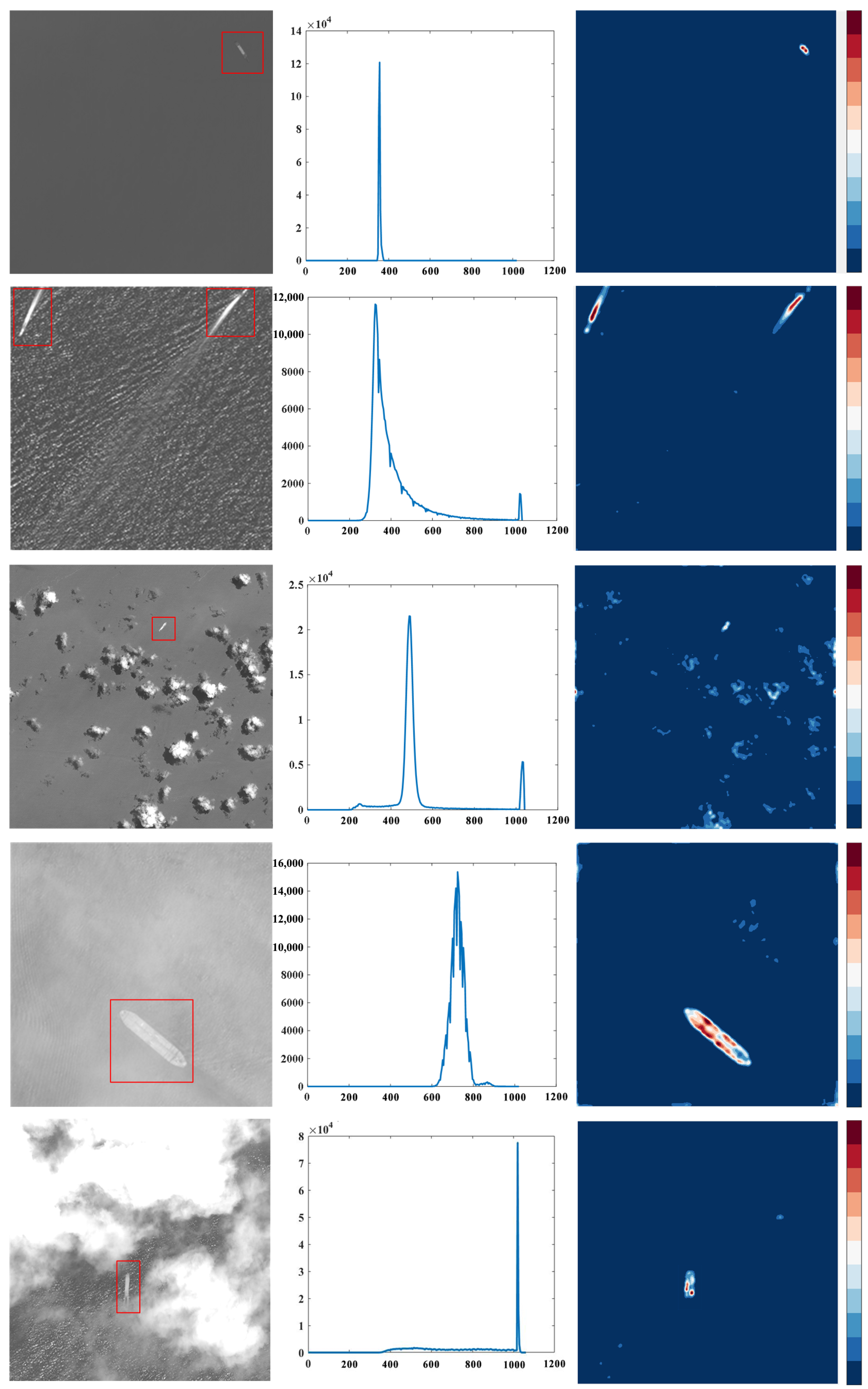
2.2. Saliency Detection for Different Scenes
2.3. Saliency Tuned YOLONet
3. Experiments
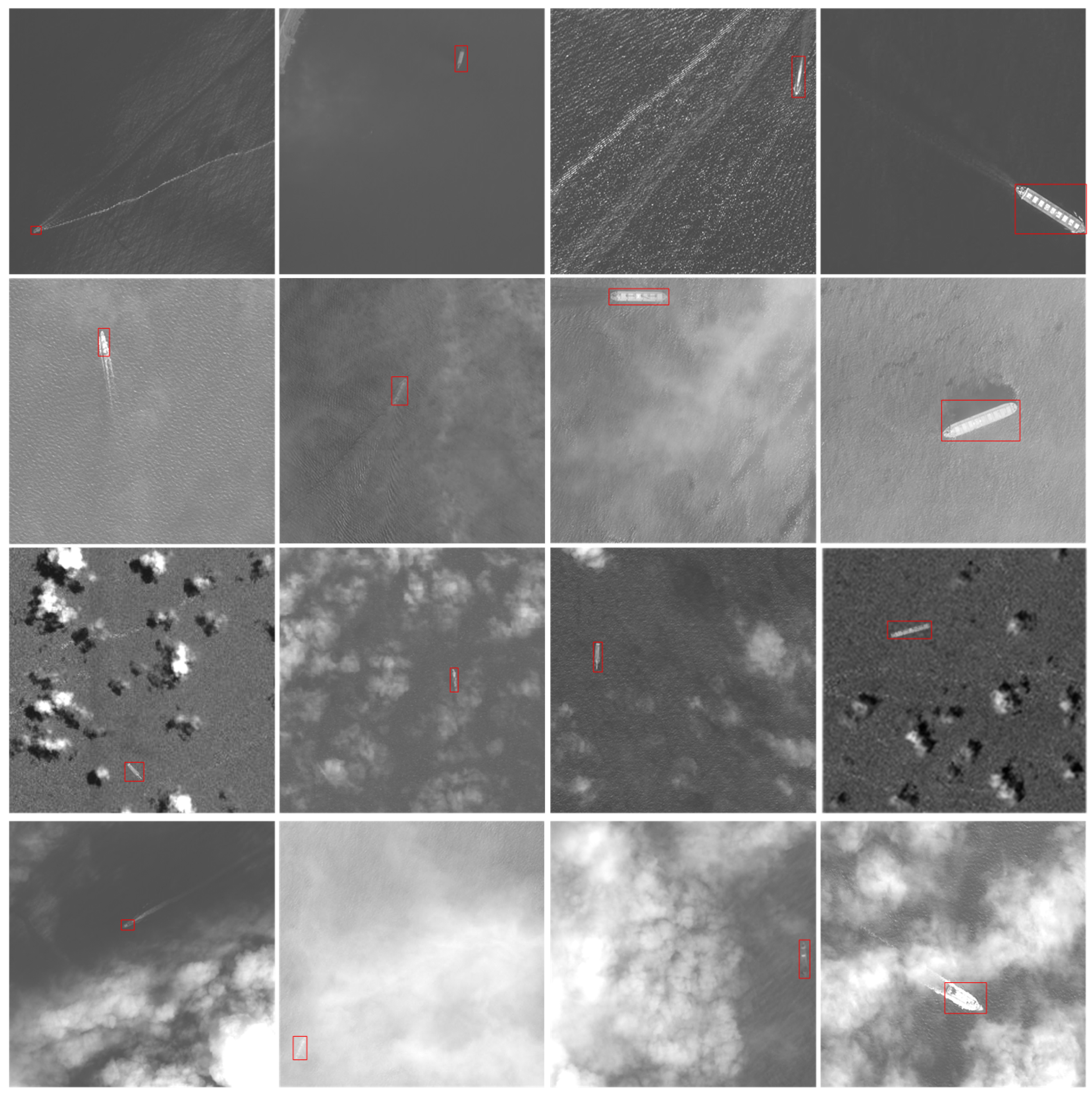
3.1. Datasets
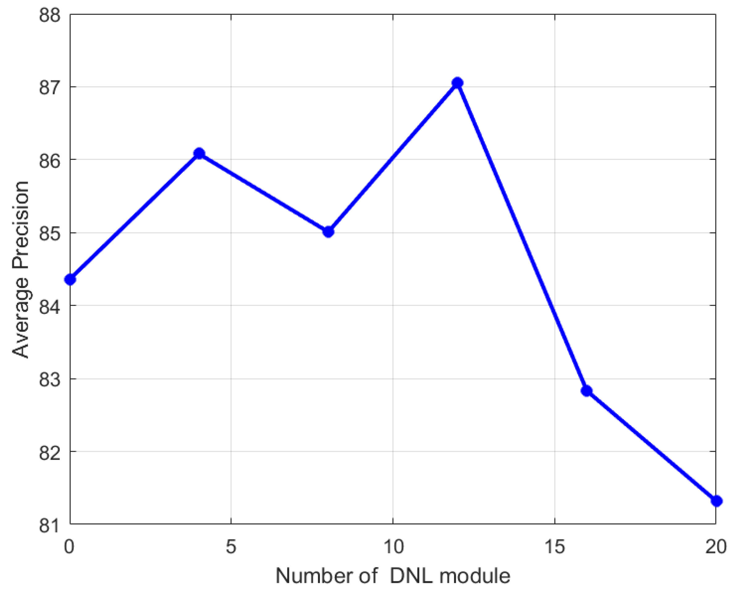
3.2. Experimental Analysis
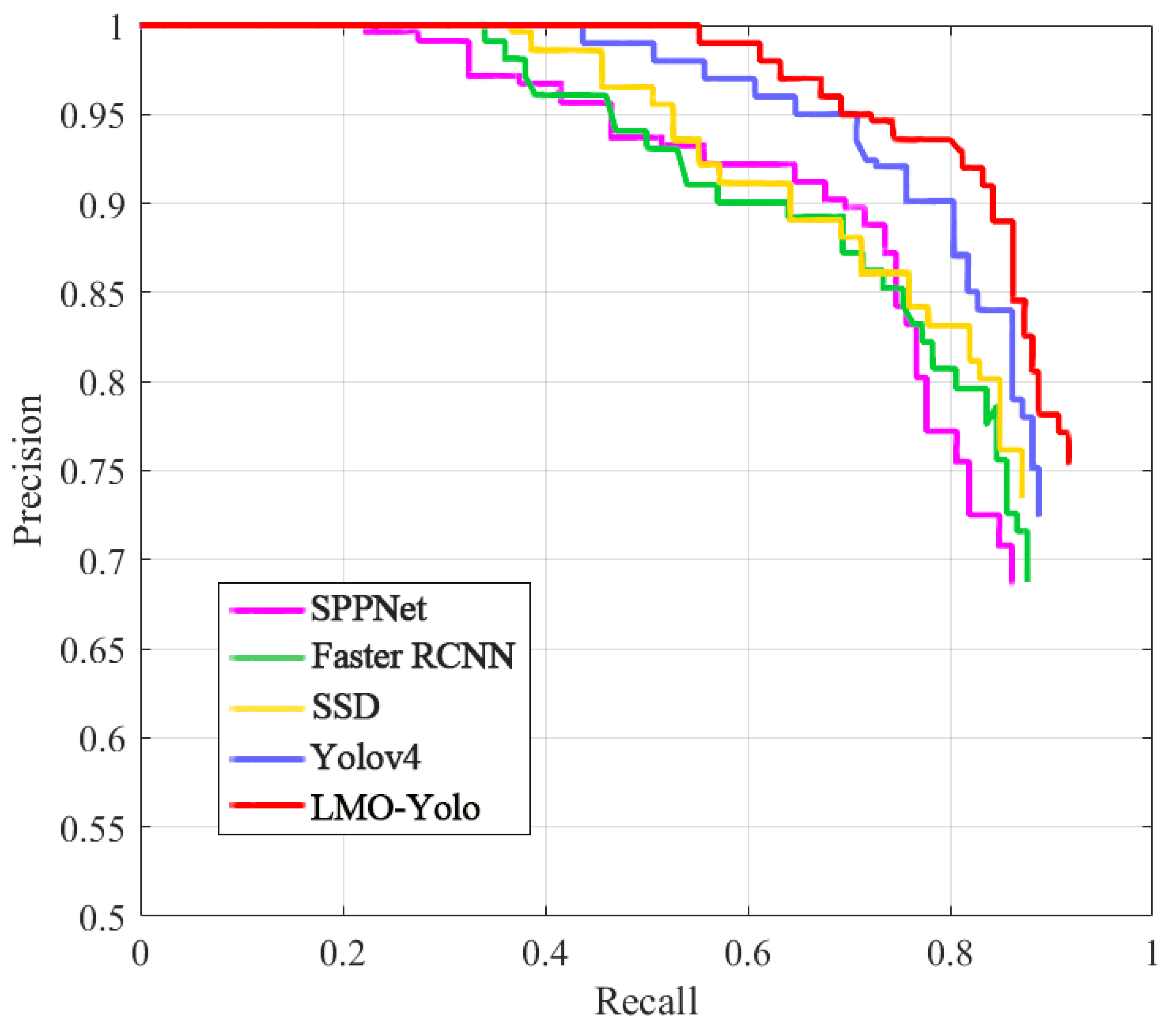
3.3. Comparisons on Detection Task with Other Methods
3.4. Discussion
4. Conclusions
Author Contributions
Funding
Institutional Review Board Statement
Informed Consent Statement
Data Availability Statement
Conflicts of Interest
References
- You, Y.; Ran, B.; Meng, G.; Li, Z.; Liu, F.; Li, Z. OPD-Net: Prow Detection Based on Feature Enhancement and Improved Regression Model in Optical Remote Sensing Imagery. IEEE Trans. Geosci. Remote Sens. 2020, 59, 6121–6137. [Google Scholar] [CrossRef]
- Hou, B.; Ren, Z.; Zhao, W.; Wu, Q.; Jiao, L. Object Detection in High-Resolution Panchromatic Images Using Deep Models and Spatial Template Matching. IEEE Trans. Geosci. Remote Sens. 2020, 58, 956–970. [Google Scholar] [CrossRef]
- Segl, K.; Kaufmann, H. Detection of small objects from high-resolution panchromatic satellite imagery based on supervised image segmentation. IEEE Trans. Geosci. Remote Sens. 2001, 39, 2080–2083. [Google Scholar] [CrossRef]
- Audebert, N.; Le Saux, B.; Lefèvre, S. How useful is region-based classification of remote sensing images in a deep learning framework? In Proceedings of the IEEE International Geoscience and Remote Sensing Symposium (IGARSS), Beijing, China, 10–15 July 2016; pp. 5091–5094. [Google Scholar] [CrossRef] [Green Version]
- Wenxiu, W.; Yutian, F.; Feng, D.; Feng, L. Remote sensing ship detection technology based on DoG preprocessing and shape features. In Proceedings of the IEEE International Conference on Computer and Communications (ICCC), Chengdu, China, 13–16 December 2017; pp. 1702–1706. [Google Scholar] [CrossRef]
- Inamdar, S.; Bovolo, F.; Bruzzone, L.; Chaudhuri, S. Multidimensional Probability Density Function Matching for Preprocessing of Multitemporal Remote Sensing Images. IEEE Trans. Geosci. Remote Sens. 2008, 46, 1243–1252. [Google Scholar] [CrossRef]
- Hurtik, P.; Molek, V.; Hula, J. Data Preprocessing Technique for Neural Networks Based on Image Represented by a Fuzzy Function. IEEE Trans. Fuzzy Syst. 2020, 28, 1195–1204. [Google Scholar] [CrossRef]
- Zheng, L.; Xu, W. An Improved Adaptive Spatial Preprocessing Method for Remote Sensing Images. Sensors 2021, 21, 5684. [Google Scholar] [CrossRef] [PubMed]
- Vivone, G.; Dalla Mura, M.; Garzelli, A.; Pacifici, F. A Benchmarking Protocol for Pansharpening: Dataset, Preprocessing, and Quality Assessment. IEEE J. Sel. Top. Appl. Earth Obs. Remote Sens. 2021, 14, 6102–6118. [Google Scholar] [CrossRef]
- Yao, J.; Fidler, S.; Urtasun, R. Describing the scene as a whole: Joint object detection, scene classification and semantic segmentation. In Proceedings of the IEEE Conference on Computer Vision and Pattern Recognition, Providence, RI, USA, 16–21 June 2012; pp. 702–709. [Google Scholar] [CrossRef] [Green Version]
- Zhong, Y.; Zhu, Q.; Zhang, L. Scene Classification Based on the Multifeature Fusion Probabilistic Topic Model for High Spatial Resolution Remote Sensing Imagery. IEEE Trans. Geosci. Remote Sens. 2015, 53, 6207–6222. [Google Scholar] [CrossRef]
- Zhu, X.X.; Tuia, D.; Mou, L.; Xia, G.S.; Zhang, L.; Xu, F.; Fraundorfer, F. Deep learning in remote sensing: A comprehensive review and list of resources. IEEE Geosci. Remote Sens. Mag. 2017, 5, 8–36. [Google Scholar] [CrossRef] [Green Version]
- Li, F.; Feng, R.; Han, W.; Wang, L. High-Resolution Remote Sensing Image Scene Classification via Key Filter Bank Based on Convolutional Neural Network. IEEE Trans. Geosci. Remote Sens. 2020, 58, 8077–8092. [Google Scholar] [CrossRef]
- Rodriguez, A.; Laio, A. Clustering by fast search and find of density peaks. Science 2014, 344, 1492–1496. [Google Scholar] [CrossRef] [PubMed] [Green Version]
- Zhu, C.; Zhou, H.; Wang, R.; Guo, J. A Novel Hierarchical Method of Ship Detection from Spaceborne Optical Image Based on Shape and Texture Features. IEEE Trans. Geosci. Remote Sens. 2010, 48, 3446–3456. [Google Scholar] [CrossRef]
- Yang, G.; Li, B.; Ji, S.; Gao, F.; Xu, Q. Ship Detection From Optical Satellite Images Based on Sea Surface Analysis. IEEE Trans. Geosci. Remote Sens. Lett. 2014, 11, 641–645. [Google Scholar] [CrossRef]
- Song, Z.; Sui, H.; Wang, Y. Automatic ship detection for optical satellite images based on visual attention model and LBP. In Proceedings of the IEEE Workshop on Electronics, Computer and Applications, IWECA, Ottawa, ON, Canada, 8–9 May 2014; pp. 722–725. [Google Scholar] [CrossRef]
- Shi, Z.; Yu, X.; Jiang, Z.; Li, B. Ship Detection in High-Resolution Optical Imagery Based on Anomaly Detector and Local Shape Feature. IEEE Trans. Geosci. Remote Sens. 2014, 52, 4511–4523. [Google Scholar] [CrossRef]
- Chen, H.; Gao, T.; Chen, W.; Zhang, Y.; Zhao, J. Contour Refinement and EG-GHT-Based Inshore Ship Detection in Optical Remote Sensing Image. IEEE Trans. Geosci. Remote Sens. 2019, 57, 8458–8478. [Google Scholar] [CrossRef]
- Hou, X.; Zhang, L. Saliency Detection: A Spectral Residual Approach. In Proceedings of the IEEE Conference on Computer Vision and Pattern Recognition, Minneapolis, MN, USA, 17–22 June 2007; pp. 1–8. [Google Scholar] [CrossRef]
- Goferman, S.; Zelnik-Manor, L.; Tal, A. Context-aware saliency detection. In Proceedings of the IEEE Computer Society Conference on Computer Vision and Pattern Recognition, San Francisco, CA, USA, 13–18 June 2010; pp. 2376–2383. [Google Scholar] [CrossRef] [Green Version]
- Tang, J.; Deng, C.; Huang, G.; Zhao, B. Compressed-Domain Ship Detection on Spaceborne Optical Image Using Deep Neural Network and Extreme Learning Machine. IEEE Trans. Geosci. Remote Sens. 2015, 53, 1174–1185. [Google Scholar] [CrossRef]
- Cheng, G.; Zhou, P.; Han, J. Learning Rotation-Invariant Convolutional Neural Networks for Object Detection in VHR Optical Remote Sensing Images. IEEE Trans. Geosci. Remote Sens. 2016, 54, 7405–7415. [Google Scholar] [CrossRef]
- Liu, L.; Ouyang, W.; Wang, X.; Fieguth, P.; Chen, J.; Liu, X.; Pietikainen, M. Deep Learning for Generic Object Detection: A Survey. Int. J. Comput. Vis. 2018, 128, 261–318. [Google Scholar] [CrossRef] [Green Version]
- Girshick, R.; Donahue, J.; Darrell, T.; Malik, J. Rich feature hierarchies for accurate object detection and semantic segmentation. In Proceedings of the IEEE Conference on Computer Vision and Pattern Recognition, Columbus, OH, USA, 23–28 June 2014; pp. 580–587. [Google Scholar]
- He, K.; Zhang, X.; Ren, S.; Sun, J. Spatial Pyramid Pooling in Deep Convolutional Networks for Visual Recognition. IEEE Trans. Pattern Anal. Mach. Intell. 2014, 37, 1904–1916. [Google Scholar] [CrossRef] [Green Version]
- Girshick, R. Fast R-CNN. In Proceedings of the IEEE International Conference on Computer Vision, Santiago, Chile, 7–13 December 2015; pp. 1440–1448. [Google Scholar]
- Ren, S.; He, K.; Girshick, R.; Sun, J. Faster RCNN: Towards real time object detection with region proposal networks. IEEE Trans. Pattern Anal. Mach. Intell. 2017, 39, 1137–1149. [Google Scholar] [CrossRef] [Green Version]
- Quiao, L.; Zhao, Y.; Li, Z.; Qiu, X.; Wu, J.; Zhang, C. DeFRCN: Decoupled Faster R-CNN for Few-Shot Object Detection. In Proceedings of the IEEE/CVF International Conference on Computer Vision, Montreal, BC, Canada, 11–17 October 2021. [Google Scholar]
- Nie, X.; Duan, M.; Ding, H.; Hu, B.; Wong, E.K. Attention Mask R-CNN for Ship Detection and Segmentation From Remote Sensing Images. IEEE Access 2020, 8, 9325–9334. [Google Scholar] [CrossRef]
- Li, Q.; Mou, L.; Liu, Q.; Wang, Y.; Zhu, X.X. HSF-Net: Multiscale Deep Feature Embedding for Ship Detection in Optical Remote Sensing Imagery. IEEE Trans. Geosci. Remote Sens. 2018, 56, 7147–7161. [Google Scholar] [CrossRef]
- Szegedy, C.; Toshev, A.; Erhan, D. Deep neural networks for object detection. In Proceedings of the Neural Information Processing Systems Conference, Lake Tahoe, NV, USA, 5–10 December 2013; pp. 2553–2561. [Google Scholar]
- Liu, W.; Anguelov, D.; Erhan, D.; Szegedy, C.; Reed, S.; Fu, C.; Berg, A. SSD: Single shot multibox detector. In Computer Vision—ECCV 2016; Lecture Notes in Computer Science; Springer: Cham, Switzerland, 2016; pp. 21–37. [Google Scholar]
- Redmon, J.; Divvala, S.; Girshick, R.; Farhadi, A. You only look once: Unified, real time object detection. In Proceedings of the IEEE Conference on Computer Vision and Pattern Recognition, Las Vegas, NV, USA, 27–30 June 2016; pp. 779–788. [Google Scholar]
- Redmon, J.; Farhadi, A. YOLO9000: Better, faster, stronger. In Proceedings of the IEEE Conference on Computer Vision and Pattern Recognition, Honolulu, HI, USA, 21–26 July 2017. [Google Scholar]
- Redmon, J.; Farhadi, A. Yolov3: An incremental improvement. arXiv 2018, arXiv:1804.02767. [Google Scholar]
- Bochkovskiy, A.; Wang, C.Y.; Liao, H.Y.M. Yolov4: Optimal speed and accuracy of object detection. arXiv 2020, arXiv:2004.10934. [Google Scholar]
- Law, H.; Deng, J. CornerNet: Detecting objects as paired keypoints. In Computer Vision—ECCV 2018; Lecture Notes in Computer Science; Springer: Cham, Switzerland, 2018; pp. 756–781. [Google Scholar]
- Chen, Q.; Wang, Y.; Yang, T.; Zhang, X.I.; Cheng, J.; Sun, J. You Only Look One-level Feature. In Proceedings of the IEEE/CVF Conference on Computer Vision and Pattern Recognition, Nashville, TN, USA, 20–25 June 2021. [Google Scholar]
- Cheng, M.-M.; Mitra, N.J.; Huang, X.; Torr, P.H.S.; Hu, S.-M. Global contrast based salient region detection. IEEE Trans. Pattern Anal. Mach. Intell. 2014, 37, 569–582. [Google Scholar] [CrossRef] [Green Version]
- Yin, M.; Yao, Z.; Cao, Y.; Li, X.; Zhang, Z.; Lin, S.; Hu, H. Disentangled non-local neural networks. In Computer Vision—ECCV 2020; Lecture Notes in Computer Science; Springer: Cham, Switzerland, 2020. [Google Scholar]
- Zheng, J.; Xu, Q.; Chen, J.; Zhang, C. The on-orbit noncloud-covered water region extraction for ship detection based on relative spectral reflectance. IEEE Geosci. Remote Sens. Lett. 2018, 15, 818–822. [Google Scholar] [CrossRef]
- Kisantal, M.; Wojna, Z.; Murawski, J.; Naruniec, J.; Cho, K. Augmentation for small object detection. arXiv 2019, arXiv:1902.07296. [Google Scholar]


| − | Scene Classification | Object Detection |
|---|---|---|
| Data size Data type | 1 × 256 Gray vector | 512 × 512 Panchromatic |
| Total samples Train samples Test samples | 2344 2110 234 | 2721 2448 273 |
| Original samples Augment samples | − − | 2245 476 |
| Methods | Baseline | SC | SD | DNL | P(%) | R(%) | AP(%) |
|---|---|---|---|---|---|---|---|
| 1 | ✓ | - | - | - | 90.77 | 80.30 | 85.21 |
| 2 | ✓ | - | ✓ | - | 91.96 | 80.65 | 85.65 |
| 3 | ✓ | - | - | ✓ | 92.37 | 81.33 | 85.82 |
| 4 | ✓ | - | ✓ | ✓ | 92.74 | 81.88 | 86.59 |
| 5 | ✓ | ✓ | ✓ | ✓ |
| Algorithm | P(%) | R(%) | AP(%) |
|---|---|---|---|
| Our approach | |||
| YOLOv4 | 90.77 | 80.30 | 85.21 |
| SSD | 84.98 | 77.76 | 81.33 |
| Faster-RCNN | 83.59 | 76.49 | 80.59 |
| SPPNet | 88.32 | 75.22 | 79.46 |
Publisher’s Note: MDPI stays neutral with regard to jurisdictional claims in published maps and institutional affiliations. |
© 2022 by the authors. Licensee MDPI, Basel, Switzerland. This article is an open access article distributed under the terms and conditions of the Creative Commons Attribution (CC BY) license (https://creativecommons.org/licenses/by/4.0/).
Share and Cite
Guo, J.; Wang, S.; Xu, Q. Saliency Guided DNL-Yolo for Optical Remote Sensing Images for Off-Shore Ship Detection. Appl. Sci. 2022, 12, 2629. https://doi.org/10.3390/app12052629
Guo J, Wang S, Xu Q. Saliency Guided DNL-Yolo for Optical Remote Sensing Images for Off-Shore Ship Detection. Applied Sciences. 2022; 12(5):2629. https://doi.org/10.3390/app12052629
Chicago/Turabian StyleGuo, Jian, Shuchen Wang, and Qizhi Xu. 2022. "Saliency Guided DNL-Yolo for Optical Remote Sensing Images for Off-Shore Ship Detection" Applied Sciences 12, no. 5: 2629. https://doi.org/10.3390/app12052629