Mining the Frequent Patterns of Named Entities for Long Document Classification

Abstract

Nowadays, a large amount of information is stored as text, and numerous text mining techniques have been developed for various applications, such as event detection, news topic classification, public opinion detection, and sentiment analysis. Although significant progress has been achieved for short text classification, document-level text classification requires further exploration. Long documents always contain irrelevant noisy information that shelters the prominence of indicative features, limiting the interpretability of classification results. To alleviate this problem, a model called MIPELD (mining the frequent pattern of a named entity for long document classification) for long document classification is demonstrated, which mines the frequent patterns of named entities as features. Discovered patterns allow semantic generalization among documents and provide clues for verifying the results. Experiments on several datasets resulted in good accuracy and marco-F1 values, meeting the requirements for practical application. Further analysis validated the effectiveness of MIPELD in mining interpretable information in text classification.

1. Introduction

Text classification is a classic topic in the field of natural language processing. With the development of information technology, a large amount of document-level text data have emerged on different topics, such as news articles [1], patent documents [2], e-commerce [3], construction specification [4], and medical narratives [5]. Effective classification of those long documents is beneficial to the efficient acquisition of target information. Differently from short texts, long documents have more characters and contain more topically irrelevant information, which usually affects text classification tasks. The core information in the document’s text is often hidden in several keywords or sentences, as shown in Figure 1. Hence, how to excavate this information is a challenging problem for long document classification.

Current mainstream methods of text classification can be divided into two categories, i.e, machine learning-based methods and deep learning-based methods. Both of them generally follow a 2-stage paradigm: Firstly, converting text data to vectors which contain the key information of text, and secondly feeding them into the classification model. How to construct a vector containing the key features of a long document is a key step to improving classification performance. For machine learning-based methods, statistics-based text representation methods are the most commonly used, such as one-hot [6], bag-of-words [7], and n-grams with TF-IDF [8]. These methods are simple and effective, with low computational costs. However, they often suffer from data sparsity, have dimensional disasters, and ignore the semantic information, especially when the text is long and contains a lot of information. Deep learning-based methods typically employ a neural network-based approach, such as word vector, which transforms the text into a low-dimensional vector. In addition, neural network models can capture more abstract semantic features between words and sentences. However, the neural network methods usually need a large scale dataset to achieve good performance, and their time consumption is significant. Besides, they are generally considered black-box models, so they are not well interpretable.

Motivated by a novel software test case recommendation method [9], which utilizes a correlation identification method to identify and recommend the proper test cases in the test case knowledge graph, we demonstrate a long document classification model, MIPELD. Our work aims to mine the core features and find the keywords in a long document. Specifically, we first apply the named entity recognition pattern to the text in preprocessing, replacing the specific name of each entity in the text with a unified entity label. This process can enhance the robustness of the extracted features for generalization among various documents. Different from [9], we adapt a distance constraint function adapted to the Apriori algorithm to mine the frequent itemsets of words which contain local features hidden in the key sentences. Furthermore, all the words and frequent itemsets are further screened as the feature words under the direction of the information gain metrics calculated using the “one vs. rest” method since the document types in long document classification tasks are pretty numerous. Subsequently, based on the selected words and frequent itemsets, all the text is converted into a discrete vector by bag-of-words. Finally, we employ a simple and effective model, a Naive Bayesian model, as the classification model. In addition, according to the selected key frequent itemsets and the feature weight of the Naive Bayesian, MIPELD provides the key sentences of each text, which can improve the interpretability of the classification results.

To summarize, our major contributions can be grouped into three parts:

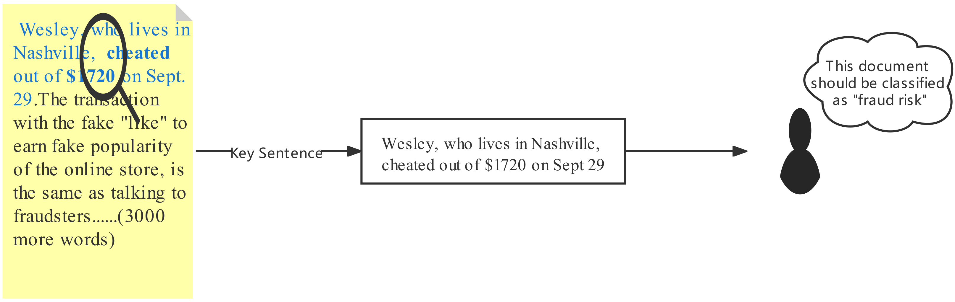
• We present the idea that identifying key information in long documents is the key to classifying such long documents;
• We demonstrate the MIPELD, a model that can extract key information from long document samples, classify them according to key information, and provide the basis for the classification choices;
• Our experimental results on three datasets demonstrate that our method has accurate and robust performance.

2. Related Work

In this section, we introduce the related work under two mainstream branches: machine learning-based methods and deep learning-based methods.

2.1. Machine Learning-Based Methods

With the development of machine learning, text classification started to utilize machine learning methods, such as Naive Bayesian (NB) [10,11,12,13,14], support vector machines (SVM) [15,16,17,18,19,20], k-nearest neighbors (KNN) [21,22,23,24,25,26], decision trees (DT) [27,28,29], and random forest (RF) [30,31,32,33].

For an NB classifier, A. Mccallum and K. Nigam [13] described the differences and details between a Bayesian network and a polynomial model which made the Naive Bayesian assumptions, and compared their classification performances on five text corpora. K. Sang-Bum et al. [12] proposed some effective techniques for Naive Bayesian text classification, which use two empirical heuristics: per-document text normalization and a feature weighting method. Z. Qu et al. [14] proposed an improved Bayes method for Chinese information classification, which applies TF-IDF into its conditional probability and applies grade factor feature weights into the classification formula of Naive Bayes.

For an SVM classifier, Z. Wang et al. [19] proposed an optimal SVM-based text classification algorithm, using multiple optimal strategies, such as the weight definition, the entropy weighting scheme for feature selection, and optimal parameter settings. M. Goudjil et al. [20] reported the active learning approach, employing SVM to select a set of documents to reduce the labeling effort.

For a KNN classifier, E.-H. Han et al. [24] proposed a weight adjusted k-nearest neighbor (WAKNN) classification model, which gains feature weights with a greedy hill climbing method. S. Jiang et al. [25] presented an improved KNN model for text categorization that combines a constrained one-pass clustering algorithm and KNN text classification. S. Chen et al. [26] presented a method of representative sample optimization based on the CURE algorithm, and proposed a quick QKNN (Quick k-nearest neighbor) on the basis of gaining the k-nearest neighbor samples.

For DT and RF classifier, B. Xu et al. [32] proposed an improved random forest algorithm for text classification and developed a novel feature weighting method and tree selection method to make the random forest model well suited to document categorization, using dozens of topics. The extreme gradient boosting (XGBoost) [34] algorithm proposed by Chen et al. an the improvement on a gradient boosting decision tree (GBDT) algorithm, which has the advantages of regularization, parallelization, and flexibility; and its performance is remarkable. The light gradient boosting machine [35] (LGB) is another improvement on the GBDT algorithm, which has several advantages, such as high accuracy and fast training speed. The decision trees in LightGBM are grown leaf-wise, instead of checking all the previous leaves for each new leaf.

These methods have performed well in text classification and showed robustness, so many researchers still use them in many fields, such as spam filtering [36] and information retrieval [37]. However, it is worth noting that machine learning-based models cannot extract features directly from text data, so they generally incorporate text representation approaches, such as bag-of-words (BOWS) [7] with n-grams [38]. Such traditional statistical-based representation approaches only employ a word frequency method to get the text representations, without considering the semantic relationships between words, which leads to the problem of data sparsity and dimensionality.

2.2. Deep Learning-Based Methods

Deep learning-based methods employ the neural-network structure, which can generate low-dimensional vectors to represent text and capture better semantic relationships between words than the statistical methods [39]. Deep learning-based methods usually use the distributed representations of words, sentences, and documents, such as Word2Vec [40] and Doc2Vec [41]; and some studies [42,43] fed the word representations obtained by these two methods into the classifier to accomplish the text classification task. The early deep learning methods for text classification used convolutional neural networks (CNN). Kim [44] proposed a convolutional neural network model called TextCNN to analyze movie reviews [45], Stanford Sentiment Treebank [46], and customer reviews [47]. TextCNN produces good results in short text classification. Other experiments [48] show that when the text length exceeds 2000, the performance of TextCNN is not significantly improved compared with the traditional methods. TextRNN [49] is a well-known text classification model; however, it is not effective at handling long documents because a long text leads to a vanishing gradient. The author also proposed a recurrent neural network (RNN) for text classification to capture contextual information. Based on long short term memory (LSTM) [50], Miwa M et al. [51] proposed an end-to-end model to classify the entity relationships in long texts. RNN and LSTM both have no restriction on text length, but they have difficulty in learning long-range correlations of sequences, and their training is time consuming. The current best systems for text classification leverage transformer-based pretrained language models [52], such as BERT [53], as a critical encoding component to achieve state-of-the-art performance. Unfortunately, transformer-based models are incapable of processing long documents due to their quadratically increasing memory and time consumption. Consequently, most transformer-based models have a length limit of 512, and recent works [54,55,56,57,58,59,60] have been devoted to alleviating this constraint. They provided several solutions for this problem:

• The truncation method [54,56]: These solutions only use some (head or tail) of the tokens from the text instance, which will lose information but reduce the computational cost.
• The hierarchical structure method [57,58,59]: A long document will be split into multiple parts to fit the length limit, and the representations of the parts are sent into neural networks to construct final representations. A typical model, the HAN [59] proposed by Yang et al., includes two levels of attention mechanisms: word level and sentence level, which allow the model to pay more or less attention to individual words or sentences in constructing the representation of a document.
• Key sentence selection [60]: These approaches aim to select the core parts of the original text instance in an intelligent way to preserve the most relevant elements.

However, all those solutions have their own drawbacks: the truncation methods lose key information from the original text; the hierarchical structure methods inevitably fail to capture long-range dependencies of text for representation learning; the key sentence selection models are complex, and their computational cost is substantially higher than that of the truncation method. Furthermore, all of these methods suffer from poor interpretability.

3. Method

Formally, given raw data with n texts, $D_{raw}=\{t_1,t_2,\dots ,t_n\}$ with respect to a specific category C, where $t_i$ stands for the $i^{th}$ text. The task of text classification is to determine which particular category each document belongs to. In this section, we introduce the implementation details of MIPELD. The model’s architecture is shown in Figure 2. In the first stage, the selected text entities are replaced with unified entity labels using the BiLSTM-CRF model. In the second stage, an improved Apriori algorithm is utilized to obtain the frequent word sets of the text. A distance constraint function is devised to extract words that are close to each other within a certain range. Then, feature words and frequent itemsets are selected under the guidance of information gain metrics. Based on these features, each text is converted into vectors according to the word frequencies. In the third stage, we feed these vectors into the Naive Bayesian model to train a classifier.

3.1. Named Entity Recognition for Semantic Generalization

Entity information in text is important for text classification. However, the number and classes of entities in long document are so numerous that the constructed text vectors will be sparse if they are selected as features directly. Hence, we leverage named entity recognition to process the text. Specifically, to obtain the entity information in the original text, we use a model incorporating bidirectional long short term memory and a conditional random field layer (BiLSTM-CRF) [61] to obtain the representation of a word with its left and right context and produce a valid sequence of output labels. Finally, we replace the entity names with the entity labels, as shown in Figure 3.

The BiLSTM layer is calculated as follows:

$$\begin{array}{c}\hfill h_t=BiLSTM[h_{t-1}:x_t]\end{array}$$

(1)

In the CRF layer, for an input text sequence $\mathbf{X}$, the score of the sequence of predictions $\mathbf{y}$ is calculated as in Equation (2):

$$s(\mathbf{X},\mathbf{y})=\sum _{i=0}^n{A}_{y_i,y_{i+1}}+\sum _{i=1}^n{P}_{i,y_i}$$

(2)

where $A_{i,j}$ is the transition matrix learned with, which represents the score of a transition from the tag i to tag j. $P_{i,j}$ is the matrix of scores output by the BiLSTM network.

3.2. Key Feature Mining

For the feature words of a long document, we should not only emphasize the keywords, but also emphasize the similar context words. To this end, we employ an improved Apriori algorithm to obtain the keywords and their contextual information close to them. At the same time, we utilize the information gain metrics as the evaluation criteria for word feature selection.

3.2.1. The Improved Apriori Algorithm

The Apriori algorithm [62] is a typical frequent itemset mining algorithm proposed by Agrawal and Srikant, which aims at discovering relationships between items in a large amount of data. Intuitively, it can find the sets of words that co-occur frequently in the text, which are the key features needed for text classification. The general procedure of Apriori is shown in Algorithm 1:

Algorithm 1: Apriori algorithm.

INPUT:  the word segmentation of text $D_{seg}$,minimum support threshold ${\theta }_{minsupport}$ OUTPUT:  Frequent itemsets of words F 1: $F_1=find\_frequent\_itemset\left(D_{seg}\right)$ 2: for($k=2;F_{k-1}!=⌀;k++)$ 3:  { 4:    $C_k=apriori\_gen\left(F_{k-1}\right)$ 5:    $F_k=\{c_k\in C_k\mid c_k.count\ge {\theta }_{minsupport}\}$ 6:  } 7: Return $F={\cup }_k{F}_k$

$F_k$ means a frequent itemset containing k items, i.e., frequent k-itemset. $C_k$ represents the candidate frequent k-itemset. Specifically, we firstly apply data cleaning methods to the sample data (removing deactivated words and irrelevant symbols, etc.), and then divide each text into words. The obtained words are considered to be itemsets, and the Apriori algorithm is applied to obtain frequent itemsets. The frequent itemsets obtained by the Apriori algorithm are the globally frequent itemsets of the text, which cannot capture the local contextual features of the keywords. Hence, we devised a distance constraint function to filter the frequent itemsets. Specifically, for a frequent itemset $F_k^l$={$w_1^l$,$w_2^l$…$w_k^l$}, we calculate the distance $dis{t}_{i,j}$ between $w_i^l$ and $w_j^l$ in $F_k^i$. For all i and j, if $dis{t}_{i,j}$ satisfies the following distance function condition (3):

$$\begin{array}{c}\hfill dis{t}_{i,j}\le k\ast lo{g}_2\lambda ,\end{array}$$

(3)

then $F_k^i$ will be selected as a feature item. k denotes the number of words contained in $F_k$. $\lambda$ is the manual hyper parameter.

3.2.2. The Information Gain

Information gain (IG) can be widely leveraged in feature selection. It implies the contributions of specific features and provides interpretable clues explicitly with respect to the classification results. Formally, the information gain is calculated as the difference between the information entropy and the conditional entropy of the dataset. Specifically, for a given corpus D consisting of K different types of text, its information entropy is calculated as in formula (4):

$$\begin{array}{c}\hfill H\left(D\right)=-\sum _{i=1}^K\frac{|C_i|}{\left|D\right|}lo{g}_2\frac{|C_i|}{\left|D\right|}\end{array}$$

(4)

where $\left|D\right|$ denotes the number of texts; |$C_i$| denotes the amount of $i^{th}$ type of text. In particular, we adopt the “one vs. rest” method to calculate the conditional entropy. The “one vs. rest” method is given n classes, including any classes as one type and other $n-1$ classes as one type, as shown in Figure 4. They are regarded as two types as input to the IG calculation process.

Then, the conditional entropy of a feature F on $C_i$ can be measured by formula (5):

$$\begin{array}{cc}\hfill H\left(C_i\right|F)& =\sum _{i=1}^{n}p\left(f\right)H\left(C_i\right|F=f)\hfill \\ & =-\sum _{f=0,1}p\left(f\right)\sum _{c=0,1}p\left(c\right|f)log\left(p\left(c\right|f)\right)\hfill \end{array}$$

(5)

c and f take the value of 1 or 0, representing the appearance and nonappearance of feature F, respectively. Finally, the information gain of feature F in one type can be measured by formula (6):

$$\begin{array}{c}\hfill IG(F,C_i)=H\left(D\right)-H\left(C_i\right|F)\end{array}$$

(6)

In this way, given training data D with n types of text, we can obtain n lists containing the value of the information gain of each candidate feature from each type of text. Next, we extract $topK$ items from the corresponding list as feature words according to the proportion of each type of text in D, so that we can get a feature word list $W_f\in \left|V\right|$. Finally, each text in D can be transformed into an $\left|V\right|$-dimensional vector by the bag-of-words model according to the $W_f$. These vectors can be used to train a classifier.

3.3. The Naive Bayesian Classifier

The main idea of our method is to identify text types based on whether the text contains key features, and the idea of the Naive Bayesian classifier coincides with it. Naive Bayesian methods have been widely used for text classification since the 1950s. Formally, given a text $t_i$, the probability of each type $c_j$ is calculated as in formula (7):

$$\begin{array}{c}\hfill p\left(c_j\right|t_i)=\frac{p\left(t_i\right|c_j)·p\left(c_j\right)}{p\left(t_i\right)}\end{array}$$

(7)

As $p\left(t_i\right)$ is the same for all types, $type\left(t_i\right)$, the type of $t_i$, can be determined by:

$$\begin{array}{cc}\hfill type\left(t_i\right)& =arg\underset{c_j}{max}\left\{p\left(c_j\right|t_i)\right\}\hfill \\ \hfill & =arg\underset{c_j}{max}\left\{p\left(t_i\right|c_j)p\left(c_j\right)\right\}\hfill \end{array}$$

(8)

Specifically, we utilize the multinomial Naive Bayesian model for text classification in this paper. In the multinomial model, a text is regarded as a bag of words. The frequency of each feature word in the text is captured. In this model, a similar Naive Bayes assumption is made: that the probability of the occurrence of each feature word in a text is independent of the occurrence of other feature words in the text. Denote the number of times feature $f_k$ occurs in text $t_i$ as $n_{ik}$; then the probability $p\left(t_i\right|c_j)$ can be computed by formula (9):

$$\begin{array}{c}\hfill p\left(t_i\right|c_j)=p\left(\right|t_i\left|\right)|t_i|!\prod _{k=1}^{\left|V\right|}\frac{p{\left(f_k\right|c_j)}^{n_{ik}}}{n_{ik}!}\end{array}$$

(9)

where $|t_i|$ is the number of feature words in text $t_i$. Given a training set D, the probability $p\left(c_j\right)$ is estimated as:

$$\begin{array}{c}\hfill p\left(c_j\right)=\frac{1+n_{c_{j}k}}{n_{all}+l}\end{array}$$

(10)

where $n_j$ is the number of texts of type $c_j$, l is the number of types, and $n_{a}ll$ is the number of all entities in $Dj$. $p\left(f_k\right|c_j)$ is computed as:

$$\begin{array}{c}\hfill p\left(f_k\right|c_j)=\frac{1+N_{c_{j}k}}{N_{all}+N_j}\end{array}$$

(11)

where $N_j$ is the number of words in class $c_j$, $N_{c_{jk}}$ is the number of words $w_k$ in class $c_j$, and $N_{all}$ is the number of words in the whole training set D.

4. Experiments

In this section, we introduce the datasets, experimental setup, and contrast methods, and report the results of the experiments. Meanwhile, to verify the effectiveness of the method, we provide analytical experiments and case analysis.

4.1. Dataset and Experimental Settings

Our experiments were conducted on several open source datasets, CCKS 2021, CCF-BDCI 2020, and THUNews. The CCKS 2021 dataset is a financial risk detection dataset containing 6000 texts from public news and reports. Each text has two classification levels: level1 is 3-tiered for risk categories, and level2 is multi-tiered for risk causality. CCF-BDCI 2020 is a news dataset containing 7320 texts with 10 classes. The THUNews dataset is a large scale news dataset which contains 836,075 instances with 14 classes. Detailed information about the datasets is shown in

Table 1. The statistics of the three datasets.

Dataset	Texts	Classes	Train	Test
CCKS 2021-Level1	6000	3	4800	1200
CCKS 2021-Level2	6000	8	4800	1200
CCF-BDCI 2020	7320	10	5856	1464
THUNews	836,075	14	668,860	167,215

. The length statistics of the texts in these two datasets are shown in Figure 5. Obviously, the average lengths of texts in CCF-BDCI 2020 and THUNews are longer than that in CCKS 2021.

In this paper, we implemented MIPELD in Python 3.7.0. Besides, several ready-made toolkits were also involved: Jieba toolkit (the Jieba toolkit is available at https://github.com/fxsjy/jieba) (accessed on 13 January 2022) for word segmentation, and Sklearn (the SKlearn toolkit is available at https://scikit-learn.org) (accessed on 13 January 2022) for the Naive Bayesian classifier. As introduced in Section 3, some hyper parameters would influence the performance. In the first stage, we substituted the following entities: name, address, organization, and time. In the key feature mining stage, we set the distance constraint parameter as 20, and the minimum support of Apriori algorithm was set to 0.2. In addition, the key feature number was set to 2000, and all datasets were randomly separated according to the text length distribution. The training data and test data were acquired by splitting the data 4:1.

4.2. Baseline Methods

To evaluate the performance of MIPELD, representative text classification models were chosen as our baselines.

4.2.1. Traditional Machine Learning Methods

• K-nearest neighbor (KNN) [21] is a non-parametric classification method that finds the k-nearest neighbors of the text to be classified in the training set, then ranks the candidate types of the text to be classified based on the neighbor types, and finally selects the type with the highest score as the type of text to be classified.
• A support vector machine (SVM) [15] is defined over the vector space where the classification problem is to find the decision surface that “best” separates the data points of one type from the other.
• A decision tree (DT) [27] creates a tree based on the attributes for categorized data points.
• Random forest (RF) [30] is an ensemble learning method for text classification, which uses multiple decision trees.
• Extreme gradient boosting (XGBoost) [34] is an improvement on the gradient boosting decision tree algorithm. It uses a novel regularization technique to control the overfitting.
• Light gradient boosting machine (LGB) [35] is another improvement on the GBDT algorithm. The decision trees in LGB are grown leaf-wise, instead of checking all the previous leaves for each new one.

In addition, all the traditional machine learning-based methods utilized the TF-IDF method for their text representation.

4.2.2. Deep Learning-Based Methods

• Word2Vec-based classification methods [42] utilize distributed representations of natural words, Word2Vec. Each word in the vocabulary is represented as a vector in a high-dimensional space. Words with similar meanings are close in vector space.
• Doc2Vec-based classification methods [43] employ Doc2Vec to represent the document, which is an unsupervised algorithm that learns vector representations of documents.
• TextCNN [44] applies convolutional neural networks (CNN) with different kernel sizes to extract different features for text classification.
• A recurrent neural network (RNN) [49] is a powerful method for text, string, and sequential data classification by assigning more weights to the previous data points of a sequence.
• Long short-term memory (LSTM) [50] is a special type of RNN that addresses text classification by preserving long term dependency in a more effective way in comparison to the basic RNN.
• BiLSTM [63] is built on LSTM, adding a backward LSTM, to encode information from back to front to obtain the semantics of the full text.
• HAN [59] is a hierarchical attention network for document classification. The HAN constructs word-level and sentence-level features, respectively. The attention mechanism is applied to assign weights to different words and sentences.
• BERT [57] is a pre-trained language model proposed by Google that extracts the semantics of texts. When dealing with long documents, we use truncation methods to get tokens for BERT.

For the Word2Vec-based and Doc2Vec-based classification methods, we employed Word2Vec and Doc2Vec, respectively, to obtain the vector representations of the documents, and utilized the Naive Bayesian classifier to obtain the classes of the documents. Finally, the classification performance was measured by accuracy rate (ACC) and marco-F1 score.

4.3. Experiments Results

4.3.1. Main Results

The experiment results are presented in

Table 2. The main results on the datasets. The best results are in bold, and the second best ones are underlined.

Model	CCKS 2021-Level1		CCKS 2021-Level2		CCF-BDCI 2020		THUNews
	ACC (%)	Macro-F1 (%)	ACC (%)	Macro-F1 (%)	ACC (%)	Macro-F1 (%)	ACC (%)	Macro-F1 (%)
KNN	59.75	38.48	42.92	31.79	88.52	87.26	84.85	82.95
RandomForest	84.58	56.55	52.25	39.38	88.80	88.00	81.01	72.04
DT	80.42	53.76	50.16	42.26	86.48	85.68	81.61	77.66
SVM	89.25	59.70	55.67	41.54	91.39	90.38	85.41	70.82
XGBoost	89.19	61.38	62.17	52.26	88.91	88.61	82.83	84.36
LGB	90.42	63.12	61.84	54.13	89.92	90.81	84.59	85.69
Word2Vec	71.42	50.80	38.50	30.94	80.19	77.82	70.36	62.87
Doc2Vec	80.17	53.91	50.08	42.12	89.84	88.34	85.57	83.13
RNN	85.50	57.17	38.60	25.27	75.27	69.63	78.40	63.98
TextCNN	89.40	59.73	58.40	46.39	86.58	84.17	92.41	90.67
UniLSTM	88.60	59.26	46.30	33.96	55.27	42.21	84.56	66.22
BiLSTM	89.20	59.67	61.80	52.09	88.01	86.50	93.05	90.44
HAN	74.73	50.15	44.87	36.47	70.75	51.88	90.36	87.27
BERT	92.70	66.96	37.80	16.56	30.74	20.85	50.63	48.84
MIPELD	89.42	68.17	62.33	55.11	92.01	90.84	87.97	85.88

. Firstly, it shows that the SVM and the two well fine-tuned models, XGBoost and LGB, outperformed the other traditional machine learning methods. Regarding the best ACC and marco-F1 they achieved, SVM achieved 91.29% and 90.38% on CCF-BDCI 2020, and 85.41% and 70.82% on THUNews, respectively. The XGBoost achieved 62.17% and 52.26% on CCKS 2021-Level2, respectively. Additionally, the LGB achieved 90.42% and 63.12%, respectively. In addition, the comparison of the experimental results on CCF-BDCI 2020 and THUNews shows that the performances of the traditional machine learning-based methods declined when the types of text in the dataset became more numerous.

Secondly, the BERT worked better than other deep learning-based methods on CCKS 2021-Level1. Regarding ACC and marco-F1, it achieved 92.70% and 66.96%, respectively. However, its performance on CCKS 2021-Level2, CCF-BDCI 2020, and THUNews was extremely poor. The reason for the poor performance of BERT on CCKS 2021-Level2 was probably that the number of samples was not enough, from three types to eight types, and the reason for the poor performance on the other two datasets was probably that the text lengths in CCF-BDCI 2020 and THUNews mostly exceeded the maximum sequence length, so some useful information placed beyond the maximum length would have been discarded by truncating, causing BERT to be incapable of capturing the features of the full text. About the hierarchical approach, the HAN, it had good results on the THUNews dataset. However, it is obvious that HAN underperformed on the first two smaller datasets. Furthermore, when dealing with extremely long documents, HAN still has to truncate them, which causes semantic loss.

Thirdly, the experimental results also show that deep learning methods usually require large datasets to guarantee good performance. Their performances are superior to those of machine learning methods when the scale of the dataset is large enough.

Finally, the MIPELD outperformed the baseline models in marco-F1 on both levels of CCKS 2021. For the accuracy rate on CCKS 2021-Level1, the BERT and the LGB achieved better scores; however, MIPELD obtained acceptable results, only lower than BERT’s by around 3% and LGB around 1%. Furthermore, MIPELD achieved the best results on both CCKS 2021-Level2 and CCF-BDCI 2020. Although several deep learning-based models outperformed MIPELD on the THUNews dataset, MIPELD still achieved comparable results and outperformed all the traditional machine learning-based methods. Meanwhile, in comparison with the results of Doc2Vec and Word2Vec, the results indicate that the features mined by MIPELD are more significant. In particular, MIPELD is more advantageous on small scale datasets, which is more valuable for practical applications, because in real scenarios we often have to deal with small scale datasets. Moreover, compared with hierarchical models, MIPELD can provide more interpretability. The frequent itemsets of key features mined by MIPELD improve the confidence of its classification results.

4.3.2. Time Consumption Analysis

We compared the model training times and the inference decoding times of all the methods on the CCF-BDCI 2020 dataset, and we summarize the results in

Table 3. The running-time comparison results.

Model	Training	Inference
KNN	1.26 s	10.98 s
RandomForest	2.98 s	2.35 s
DT	4.08 s	0.78 s
SVM	16.72 s	6.26 s
XGBoost	29.62 s	4.90 s
LGB	22.17 s	5.10 s
Word2Vec	36.13 s	26.01 s
Doc2Vec	106.21 s	28.80 s
RNN	59 min	7 min
TextCNN	73 min	9 min
UniLSTM	60 min	7 min
BiLSTM	82 min	10 min
HAN	89 min	5 min
BERT	102 min	13 min
MIPELD	33.09 s	8.12 s

. The evaluation of MIPELD and traditional machine learning-based models was based on an Intel i7-10700 CPU, whereas the evaluation of deep learning-based methods was based on a single Nvidia P100 GPU.

It is obvious that the time consumed by the machine learning algorithms was less than that consumed by the deep learning algorithms. In particular, BERT had the highest time consumption due to the complexity of its architecture, and the RNN and the LSTM cannot process data in parallel, resulting in high time consumption as well. In addition, for the time consumption of Word2Vec and Doc2Vec, we only counted the training and inference time taken by the Naive Bayesian classifier, so their time consumption is on the same level as that of the traditional machine learning models. By comparing the time consumption results with baselines, we can conclude that MIPELD possesses the advantage of low time consumption, yet it has comparable classification performance.

4.4. Ablation Experiments

The key motivation of MIPELD is to extract the key local features of a long document and give interpretable grounds for classification. Specially, we utilized two components to achieve this: named entity label replacement and an improved Apriori algorithm with a distance constraint function. To evaluate the effectiveness of MIPELD, we conducted an ablation experiment, and the results are shown in

Table 4. Results of the main components ablation experiment. NER denotes the semantic generalization from the named entity recognition.

Model	CCKS 2021-Level1		CCKS 2021-Level2		CCF-BDCI 2020		THUNews
	Macro-F1 (%)	Decline↓(%)	Macro-F1 (%)	Decline↓(%)	Macro-F1 (%)	Decline↓(%)	Macro-F1 (%)	Decline↓(%)
MIPELD	68.17	-	55.11	-	90.84	-	87.96	-
w/o NER	66.27	1.90	54.54	0.57	90.66	0.18	86.88	1.08
w/o Apriori	63.31	4.86	52.98	2.13	90.46	0.38	82.36	5.60
w/o Distance	63.73	4.44	53.87	1.24	90.59	0.25	85.78	2.11

.

4.4.1. About Named Entity Label Replacement

The performance of w/o NER drops slightly in Table 4. On the one hand, it indicates that the semantic generalization of entity can boost the performance. On the other hand, the contextual semantic features of the improved Apriori algorithm can express the local features of long documents, which may be the reason for the smaller decline of the algorithm.

4.4.2. About the Improved Apriori Algorithm

Among all models, MIPELD w/o Apriori achieved the worst performance. This observation reflects that not only the individual word but also its contextual information contained in its synonyms should be emphasized for classification.

4.4.3. About the Distance Constraint Function

The distance constraint function aims to constrain the distances of words in the frequent itemsets in order to mine the local features. It is worth noting that the performance of MIPELD w/o the distance constraint function declined more on the CCF-BDCI 2020 dataset than on CCKS 2021, which might have been due to the longer length of texts in CCF-BDCI 2020 than in CCKS 2021.

4.5. Case Study

We present a case study on classification results visualization and feature weights’ contributions visualization.

4.5.1. Classification Results Visualization

Intuitively, there are some significant words in a long document to help with text classification. Another advantage of MIPELD is the by-products—the frequent itemsets obtained by the improved Apriori algorithm, which can provide interpretable evidence for classification by locating the key sentences. For example, case 1 with 3994 words in

Table 5. The key sentences. mined by MIPELD.

Class	Dataset	Frequent Itemsets Feature	Key Sentence	Original Texts
Fraud risk	CCKS 2021-Level1	“[name], [money], cheat”	[name], who lives in Nashville, was cheated out of [money] on 29 September.	Wesley, who lives in Nashville, was cheated out of $\$1720$ on 29 September. The transaction with the fake “like” to earn fake popularity of the online store, is the same as talking to fraudsters…(3000 more words)
Part-time click farming	CCKS 2021-Level2	“[name], click farming”, “[name], [money], cheat”	In the [time], [name] saw an ad in a chat group, advertising that there is a software can make a profit by part-time click farming,…, So in the end [name] was cheated out of a total of [money]	In the afternoon of 5 September 2019, Larry saw an ad in a chat group, advertising that there is a software can make a profit by part-time click farming,…, So in the end Larry was cheated out of a total of $29,686.
Sports	CCF-BDCI 2020	“[name], medalist, [time]”	On [time], [name], the bronze medalist in the singles men’s table tennis at the Rio Olympics, posted that he had resumed training.	On 22 September, Jun Mizutani, the bronze medalist in the singles men’s table tennis at the Rio Olympics, posted that he had resumed training…(500 more words).
Lottery	THUNews	“lottery, [time], [address]”	Lottery winner may have hit $80m jackpot–china’s lottery may have set a new record with a man expected to win 514 million yuan ($80 million) from two tickets bought in East China’s [address] on [time].	Lottery winner may have hit $80m jackpot–china’s lottery may have set a new record with a man expected to win 514 million yuan ($80 million) from two tickets bought in East China’s Zhejiang Proince on Tuesday...(600 more words).

was classified into “Fraud risk,” because words such as “cheated,” “$1720,” and “Wesley” were detected by MIPELD. Similarity, for case 2, which is related to money fraud for the reason of part-time click farming, the model focused its attention on such words as “Larry,” “click farming,” “cheated,” and “$29,686,” and thus classified this case into “Part-time click farming”.

4.5.2. Feature Weights’ Contributions Visualization

In this section, we analyze the weight contributions of the features mined by MIPELD based on the experimental results on the CCKS 2021dataset. Figure 6 shows the three key features with the highest contributions in each class in CCKS 2021-Level1. As shown in

Table 6. The interpretability of classification results.

Class	Original Sentences	Interpretability
Misappropriation risk	On 18 January 2019, Young, who worked in an auto equipment manufacturing company in Wuhu City, verbally reported to the police that he had identity theft on their credit card and $2900 was spent in their account…(1700 more words)	On [time], [name], who worked in an auto equipment manufacturing company in [address], verbally reported to the police that he had identity theft on their credit card and [money] was spent in their account.
Fraud risk	Wesley, who lives in Nashville, cheated out of $\$1720$ on 29 September. The transaction with the fake “like” to earn fake popularity of the online store, is the same as talking to fraudsters…(3000 more words)	[name], who lives in Nashville, was cheated out of [money] on 29 September.
Others	From February 2018 to April 2018, Cai used their cell phone for profit, disseminated obscene electronic information through online chat and other forms, disseminated more than 80 obscene videos and more than 200 obscene pictures, and made a profit of more than $9000. He was accused of spreading obscene materials…(1500 more words)	From [time] to [time], [name] used their cell phone for profit, disseminated obscene electronic information through online chat and other forms, disseminated more than 80 obscene videos and more than 200 obscene pictures, and made a profit of more than $9000. He was accused of spreading obscene materials.

, these features provide interpretability to the results of text classification.

4.6. Analysis Experiments

In this section, we further discuss the effectiveness of the distance constraint and the semantic generalization obtained from named entity recognition.

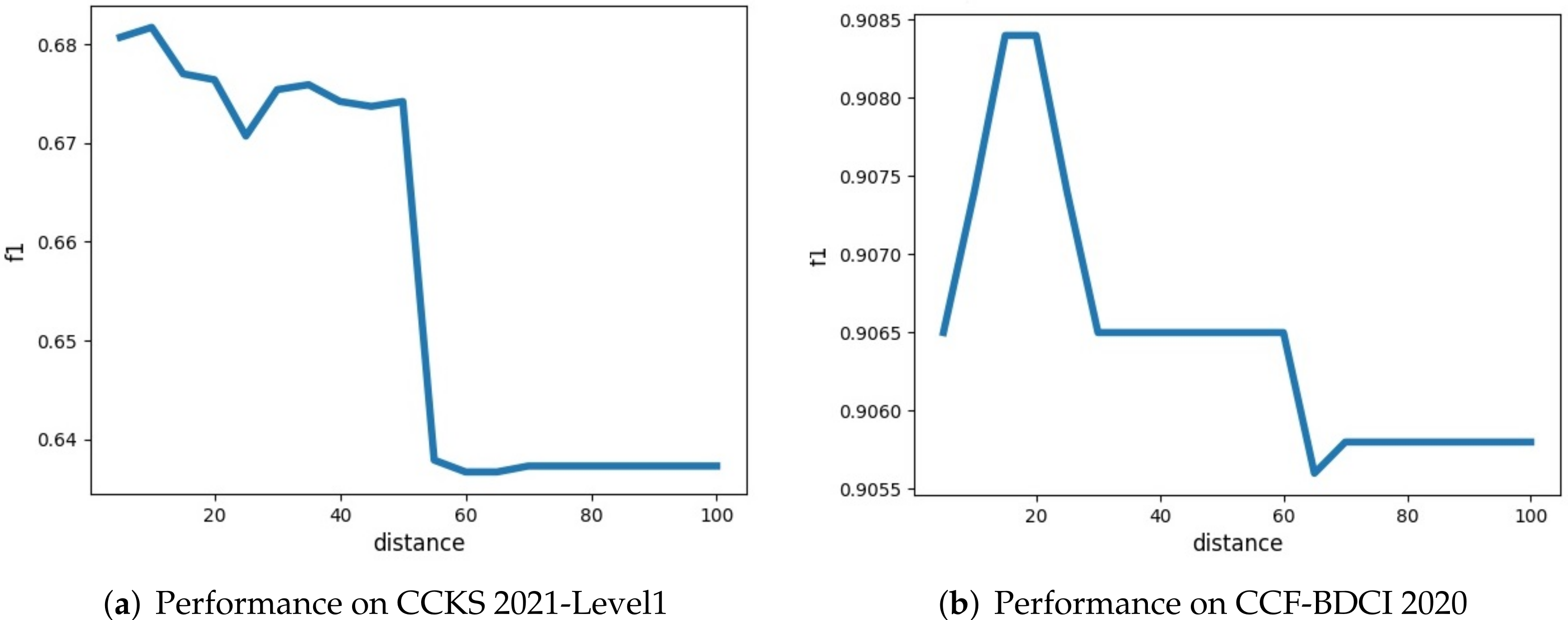
4.6.1. The Effectiveness of the Distance Constraint

In order to verify the effectiveness of the distance constraint, we firstly adjusted its parameter $\lambda$ from 5 to 100, and analyzed then the evolution of performance. Firstly, Figure 7 shows that with the increases in the distance constraint, the macro-F1 at first increased to its maximum and then decreased, and finally stayed at a stable value, which is consistent with the result of MIPELD w/o the distance constraint in the ablation experiment. The reason is that when $\lambda$ is relatively small, the distance constraint is more strict and most of the frequent itemsets are excluded; when $\lambda$ is large, the distance constraint is too lenient to filter the frequent itemsets, so it loses its effect. Moreover, we can observe that for two datasets, MIPELD achieved its best respectibe performances when $\lambda$ = 10 or $\lambda$ = 15, respectively. The possible reason is that the average text length of CCKS 2021 is shorter than that of CCF-BDCI 2020.

4.6.2. The Effectiveness of the Semantic Generalization

In this section, we investigate how the semantic generalization contributes to the classification performance.

Table 7. The effects of different entity label replacements on feature dimensionality and model performance. w/o NER means no replacement of entity label.

Replaced Entities	Feature Vector Dimensions	ACC (%)	Macro-F1 (%)
w/o NER	1227	89.33	66.27
organization	1216	89.33	67.64
organization, money, address	1117	89.37	68.11
organization, money, name, address, time	1115	89.42	68.17
organization, money, name, address, time, job	1113	88.83	67.32

demonstrates the classification performance when using different entity replacement strategies. It shows that as the number of replacement entities increased, the dimensionality of the feature vector was reduced and the model achieved better performance. This observation indicates that generalizing the semantics of entities, i.e., replacing entities with their labels, can alleviate the feature sparsity. In addition, it is worth noting that the performance decreased after replacing the “job” entities, which indicates that the “job” entities’ diversity is relevant for classification, and it also shows that the selection of the replacement entities should be based on the actual situation.

5. Conclusions

Our study proposed a novel document-level classification method that classifies documents by generalizing the semantics of named entities in the text and mining key features existing at local areas in long documents. First, various named entities in the texts are replaced with named entity labels obtained by the BiLSTM-CRF model. Second, the improved Apriori algorithm is used o mine the frequent itemsets that exist in the local parts of the documents. Meanwhile, the information gain metric is used to select the key features. Then, under the direction of the mined key features, the texts are converted to numerical vectors using the bag-of-words model. Finally, the Naive Bayesian classifier is applied to classify the text.

This research made some contributions to the task of document classification. First, this paper presents the idea of classifying long documents by local key features and their combinations, which is indeed helpful for document classification according to the experimental results. Second, we provide the document-level classification method MIPELD, which mines key features of document text that contain the frequent patterns of named entities. These key features mined by our model provide a high interpretability paradigm for classification results.

There are some improvements needed to our model. First, the optimal threshold of the distance constraint function in the improved Apriori algorithm is obtained by using grid search experiments. MIPELD would have stronger robustness if a module could be designed to adaptively generate the optimal threshold based on text length. Second, for the basis of mining key features, we have only adopted the distance between keywords so far. If we combine other constraints, such as syntactic dependency, then the key features will be more significant and will provide better interpretability. With these modules to select the replaced named entities, the classification performance will be improved.

References

1. Jang, B.; Kim, I.; Kim, J.W. Word2vec convolutional neural networks for classification of news articles and tweets. PLoS ONE 2019, 14, e0220976. [Google Scholar] [CrossRef] [PubMed] [Green Version]
2. Bai, J.; Shim, I.; Park, S. MEXN: Multi-Stage Extraction Network for Patent Document Classification. Appl. Sci. 2020, 10, 6229. [Google Scholar] [CrossRef]
3. Wang, X.; Tong, Y. Application of an emotional classification model in e-commerce text based on an improved transformer model. PLoS ONE 2021, 16, e0247984. [Google Scholar] [CrossRef] [PubMed]
4. Moon, S.; Lee, G.; Chi, S. Semantic text-pairing for relevant provision identification in construction specification reviews. Autom. Constr. 2021, 128, 103780. [Google Scholar] [CrossRef]
5. Venkataraman, G.R.; Pineda, A.L.; Bear Don’t Walk IV, O.J.; Zehnder, A.M.; Ayyar, S.; Page, R.L.; Bustamante, C.D.; Rivas, M.A. FasTag: Automatic text classification of unstructured medical narratives. PLoS ONE 2020, 15, e0234647. [Google Scholar] [CrossRef]
6. Zhang, X.; LeCun, Y. Which encoding is the best for text classification in chinese, english, japanese and korean? arXiv 2017, arXiv:1708.02657. [Google Scholar]
7. Ling, W.; Tsvetkov, Y.; Amir, S.; Fermandez, R.; Dyer, C.; Black, A.W.; Trancoso, I.; Lin, C.C. Not all contexts are created equal: Better word representations with variable attention. In Proceedings of the 2015 Conference on Empirical Methods in Natural Language Processing, Pittsburgh, PA, USA, 17–21 September 2015; pp. 1367–1372. [Google Scholar]
8. Zhang, X.; Zhao, J.; LeCun, Y. Character-level convolutional networks for text classification. Adv. Neural Inf. Process. Syst. 2015, 28, 649–657. [Google Scholar]
9. Ke, W.J.; Wu, C.; Fu, X.F.; Gao, C.; Song, Y.Y. Interpretable Test Case Recommendation based on Knowledge Graph. In Proceedings of the 2020 International Conference on Software Quality (QRS), Macau, China, 11–14 December 2020; IEEE: Macau, China, 2020; pp. 489–496. [Google Scholar]
10. Heckerman, D. Bayesian networks for data mining. Data Min. Knowl. Discov. 1997, 1, 79–119. [Google Scholar] [CrossRef]
11. Chen, J.; Huang, H.; Tian, S.; Qu, Y. Feature selection for text classification with Naïve Bayes. Expert Syst. Appl. 2009, 36, 5432–5435. [Google Scholar] [CrossRef]
12. Kim, S.B.; Han, K.S.; Rim, H.C.; Myaeng, S.H. Some effective techniques for naive bayes text classification. IEEE Trans. Knowl. Data Eng. 2006, 18, 1457–1466. [Google Scholar]
13. McCallum, A.; Nigam, K. A comparison of event models for naive bayes text classification. In AAAI-98 Workshop on Learning for Text Categorization; Citeseer: Princeton, NJ, USA, 1998; Volume 752, pp. 41–48. [Google Scholar]
14. Qu, Z.; Song, X.; Zheng, S.; Wang, X.; Song, X.; Li, Z. Improved Bayes method based on TF-IDF feature and grade factor feature for chinese information classification. In Proceedings of the 2018 IEEE International Conference on Big Data and Smart Computing (BigComp), Shanghai, China, 15–17 January 2018; IEEE: Shanghai, China, 2018; pp. 677–680. [Google Scholar]
15. Vapnik, V.; Chervonenkis, A.Y. A class of algorithms for pattern recognition learning. Avtomat. Telemekh 1964, 25, 937–945. [Google Scholar]
16. Cortes, C.; Vapnik, V. Support-vector networks. Mach. Learn. 1995, 20, 273–297. [Google Scholar] [CrossRef]
17. Haddoud, M.; Mokhtari, A.; Lecroq, T.; Abdeddaïm, S. Combining supervised term-weighting metrics for SVM text classification with extended term representation. Knowl. Inf. Syst. 2016, 49, 909–931. [Google Scholar] [CrossRef]
18. Kim, H.; Howland, P.; Park, H.; Christianini, N. Dimension reduction in text classification with support vector machines. J. Mach. Learn. Res. 2005, 6, 37–53. [Google Scholar]
19. Wang, Z.Q.; Sun, X.; Zhang, D.X.; Li, X. An optimal SVM-based text classification algorithm. In Proceedings of the 2006 International Conference on Machine Learning and Cybernetics, Dalian, China, 13–16 August 2006; IEEE: Dalian, China, 2006; pp. 1378–1381. [Google Scholar]
20. Goudjil, M.; Koudil, M.; Bedda, M.; Ghoggali, N. A novel active learning method using SVM for text classification. Int. J. Autom. Comput. 2018, 15, 290–298. [Google Scholar] [CrossRef]
21. Fix, E.; Hodges, J.L. Discriminatory analysis. Nonparametric discrimination: Consistency properties. Int. Stat. Rev. Int. Stat. 1989, 57, 238–247. [Google Scholar] [CrossRef]
22. Lu, L.R.; Fa, H.Y. A Density-Based Method for Reducing the Amount of Training Data in kNN Text Classification. J. Comput. Res. Dev. 2004, 41, 539–545. [Google Scholar]
23. Wandabwa, H.; Zhang, D.; Sammy, K. Text categorization via attribute distance weighted k-nearest neighbor classification. In Proceedings of the 2016 International Conference on Information Technology (ICIT), Bhubaneswar, India, 22–24 December 2016; IEEE: Bhubaneswar, India, 2016; pp. 225–228. [Google Scholar]
24. Han, E.H.S.; Karypis, G.; Kumar, V. Text categorization using weight adjusted k-nearest neighbor classification. In Pacific-Asia Conference on Knowledge Discovery and Data Mining; Springer: Minneapolis, MN, USA, 2001; pp. 53–65. [Google Scholar]
25. Jiang, S.; Pang, G.; Wu, M.; Kuang, L. An improved K-nearest-neighbor algorithm for text categorization. Expert Syst. Appl. 2012, 39, 1503–1509. [Google Scholar] [CrossRef]
26. Chen, S. K-nearest neighbor algorithm optimization in text categorization. In IOP Conference Series: Earth and Environmental Science; IOP Publishing: Bristol, UK, 2018; Volume 108, p. 052074. [Google Scholar]
27. Hormann, A.M. Programs for machine learning Part I. Inf. Control. 1962, 5, 347–367. [Google Scholar] [CrossRef] [Green Version]
28. Wang, Y.; Wang, Z.O. Text categorization rule extraction based on fuzzy decision tree. In Proceedings of the 2005 International Conference on Machine Learning and Cybernetics, Guangzhou, China, 18–21 August 2005; IEEE: Guangzhou, China, 2005; Volume 4, pp. 2122–2127. [Google Scholar]
29. Bahassine, S.; Madani, A.; Kissi, M. An improved Chi-sqaure feature selection for Arabic text classification using decision tree. In Proceedings of the 2016 11th International Conference on Intelligent Systems: Theories and Applications (SITA), Mohammedia, Morocco, 19–20 October 2016; pp. 1–5. [Google Scholar]
30. Breiman, L. Random forests. Mach. Learn. 2001, 45, 5–32. [Google Scholar] [CrossRef] [Green Version]
31. Parmar, H.; Bhanderi, S.; Shah, G. Sentiment mining of movie reviews using Random Forest with Tuned Hyperparameters. In Proceedings of the International Conference on Information Science, Seoul, Korea, 6–9 May 2014; pp. 1–6. [Google Scholar]
32. Xu, B.; Guo, X.; Ye, Y.; Cheng, J. An Improved Random Forest Classifier for Text Categorization. J. Comput. 2012, 7, 2913–2920. [Google Scholar] [CrossRef] [Green Version]
33. Islam, M.Z.; Liu, J.; Li, J.; Liu, L.; Kang, W. A semantics aware random forest for text classification. In Proceedings of the 28th ACM International Conference on Information and Knowledge Management, Beijing, China, 3–7 November 2019; pp. 1061–1070. [Google Scholar]
34. Chen, T.; Guestrin, C. Xgboost: A scalable tree boosting system. In Proceedings of the 22nd Acm Sigkdd International Conference on Knowledge Discovery and Data Mining, San Francisco, CA, USA, 13–17 August 2016; pp. 785–794. [Google Scholar]
35. Ke, G.; Meng, Q.; Finley, T.; Wang, T.; Chen, W.; Ma, W.; Ye, Q.; Liu, T.Y. Lightgbm: A highly efficient gradient boosting decision tree. In Proceedings of the Advances in Neural Information Processing Systems 30 (NIPS 2017), Long Beach, CA, USA, 4–9 December 2017; 30. [Google Scholar]
36. Guzella, T.S.; Caminhas, W.M. A review of machine learning approaches to spam filtering. Expert Syst. Appl. 2009, 36, 10206–10222. [Google Scholar] [CrossRef]
37. Dwivedi, S.K.; Arya, C. Automatic text classification in information retrieval: A survey. In Proceedings of the Second International Conference on Information and Communication Technology for Competitive Strategies, Udaipur, India, 4–5 May 2016; pp. 1–6. [Google Scholar]
38. Lin, C.Y.; Hovy, E. Automatic evaluation of summaries using n-gram co-occurrence statistics. In Proceedings of the 2003 Human Language Technology Conference of the North American Chapter of the Association for Computational Linguistics, Edmonton, AB, Canada, 27 May 2003; pp. 150–157. [Google Scholar]
39. Joulin, A.; Grave, E.; Bojanowski, P.; Mikolov, T. Bag of tricks for efficient text classification. arXiv 2016, arXiv:1607.01759. [Google Scholar]
40. Mikolov, T.; Sutskever, I.; Chen, K.; Corrado, G.S.; Dean, J. Distributed representations of words and phrases and their compositionality. Adv. Neural Inf. Process. Syst. 2013, 26, 3111–3119. [Google Scholar]
41. Le, Q.; Mikolov, T. Distributed representations of sentences and documents. In Proceedings of the 31st International Conference on Machine Learning, PMLR, China, Bejing, 22–24 June 2014; pp. 1188–1196. [Google Scholar]
42. Altowayan, A.A.; Tao, L. Word embeddings for Arabic sentiment analysis. In Proceedings of the 2016 IEEE International Conference on Big Data (Big Data), Washington, DC, USA, 5–8 December 2016; IEEE: Washington, DC, USA, 2016; pp. 3820–3825. [Google Scholar]
43. Dogru, H.B.; Tilki, S.; Jamil, A.; Hameed, A.A. Deep learning-based classification of news texts using doc2vec model. In Proceedings of the 2021 1st International Conference on Artificial Intelligence and Data Analytics (CAIDA), Riyadh, Saudi Arabia, 6–7 April 2021; pp. 91–96. [Google Scholar]
44. Kim, Y. Convolutional Neural Networks for Sentence Classification. In Proceedings of the 2014 Conference on Empirical Methods in Natural Language Processing (EMNLP), Doha, Qatar, 25 August 2014. [Google Scholar]
45. Pang, B.; Lee, L. Seeing stars: Exploiting class relationships for sentiment categorization with respect to rating scales. In Proceedings of the 43rd Annual Meeting of the Association for Computational Linguistics (ACL’05), Ann Arbor, MI, USA, 25–30 June 2005. [Google Scholar]
46. Socher, R.; Perelygin, A.; Wu, J.; Chuang, J.; Manning, C.D.; Ng, A.Y.; Potts, C. Recursive deep models for semantic compositionality over a sentiment treebank. In Proceedings of the 2013 Conference on Empirical Methods in Natural Language Processing, Seattle, WA, USA, 18–21 October 2013; pp. 1631–1642. [Google Scholar]
47. Hu, M.; Liu, B. Mining and summarizing customer reviews. In Proceedings of the Tenth ACM SIGKDD International Conference on Knowledge Discovery and Data Mining, Seattle, WA, USA, 22–25 August 2004; pp. 168–177. [Google Scholar]
48. Keeling, R.; Chhatwal, R.; Huber-Fliflet, N.; Zhang, J.; Wei, F.; Zhao, H.; Shi, Y.; Qin, H. Empirical Comparisons of CNN with Other Learning Algorithms for Text Classification in Legal Document Review. In Proceedings of the 2019 IEEE International Conference on Big Data (Big Data), Los Angeles, CA, USA, 9–12 December 2019; pp. 2038–2042. [Google Scholar]
49. Liu, P.; Qiu, X.; Huang, X. Recurrent neural network for text classification with multi-task learning. arXiv 2016, arXiv:1605.05101. [Google Scholar]
50. Hochreiter, S.; Schmidhuber, J. Long short-term memory. Neural Comput. 1997, 9, 1735–1780. [Google Scholar] [CrossRef]
51. Miwa, M.; Bansal, M. End-to-end relation extraction using lstms on sequences and tree structures. arXiv 2016, arXiv:1601.00770. [Google Scholar]
52. Vaswani, A.; Shazeer, N.; Parmar, N.; Uszkoreit, J.; Jones, L.; Gomez, A.N.; Kaiser, L.; Polosukhin, I. Attention is all you need. In Proceedings of the Advances in Neural Information Processing Systems, Long Beach, CA, USA, 4–9 December 2017; pp. 5998–6008. [Google Scholar]
53. Devlin, J.; Chang, M.W.; Lee, K.; Toutanova, K. Bert: Pre-training of deep bidirectional transformers for language understanding. arXiv 2018, arXiv:1810.04805. [Google Scholar]
54. Sun, C.; Qiu, X.; Xu, Y.; Huang, X. How to fine-tune bert for text classification. In China National Conference on Chinese Computational Linguistics; Springer: Hohhot, China, 2019; pp. 194–206. [Google Scholar]
55. Akbik, A.; Bergmann, T.; Blythe, D.; Rasul, K.; Schweter, S.; Vollgraf, R. FLAIR: An easy-to-use framework for state-of-the-art NLP. In Proceedings of the 2019 Conference of the North American Chapter of the Association for Computational Linguistics (Demonstrations), Minneapolis, MN, USA, 2–7 June 2019; pp. 54–59. [Google Scholar]
56. Adhikari, A.; Ram, A.; Tang, R.; Lin, J. Docbert: Bert for document classification. arXiv 2019, arXiv:1904.08398. [Google Scholar]
57. Mulyar, A.; Schumacher, E.; Rouhizadeh, M.; Dredze, M. Phenotyping of clinical notes with improved document classification models using contextualized neural language models. arXiv 2019, arXiv:1910.13664. [Google Scholar]
58. Zhang, R.; Wei, Z.; Shi, Y.; Chen, Y. BERT-AL: BERT for Arbitrarily Long Document Understanding. In Proceedings of the 8th International Conference on Learning Representations, ICLR 2020, Addis Ababa, Ethiopia, 26–30 April 2020. [Google Scholar]
59. Yang, Z.; Yang, D.; Dyer, C.; He, X.; Smola, A.; Hovy, E. Hierarchical attention networks for document classification. In Proceedings of the 2016 conference of the North American Chapter of the Association for Computational Linguistics: Human Language Technologies, San Diego, CA, USA, 12–17 June 2016; pp. 1480–1489. [Google Scholar]
60. Min, S.; Zhong, V.; Socher, R.; Xiong, C. Efficient and robust question answering from minimal context over documents. arXiv 2018, arXiv:1805.08092. [Google Scholar]
61. Lample, G.; Ballesteros, M.; Subramanian, S.; Kawakami, K.; Dyer, C. Neural Architectures for Named Entity Recognition. 2016. Available online: http://xxx.lanl.gov/abs/1603.01360 (accessed on 13 January 2022).
62. Agrawal, R.; Srikant, R. Fast algorithms for mining association rules. In Proceedings of the 20th International Conference on Very Large Data Bases, Santiago de Chile, Chile, 12–15 September 1994; Volume 1215, pp. 487–499. [Google Scholar]
63. Graves, A.; Schmidhuber, J. Framewise phoneme classification with bidirectional LSTM and other neural network architectures. Neural Netw. 2005, 18, 602–610. [Google Scholar] [CrossRef]
Figure 1. An example of a long document’s key sentences. These key sentences can be very effective in helping people to classify the document.
Applsci 12 02544 g001
Figure 2. The overview of MIPELD’s structure.
Applsci 12 02544 g002
Figure 3. An example of entity label replacement.
Applsci 12 02544 g003
Figure 4. The classification method of “one vs. rest”.
Applsci 12 02544 g004
Figure 5. The text length statistics of datasets. The c-axis in the figure represents the length of text, and the y-axis represents the quantity of text. Obviously, the average lengths of texts in CCF-BDCI 2020 and THUNews are longer than that of CCKS 2021. Specifically, the average lengths in the three datasets are 592.2, 969.6, and 941.4; and the medians are 289, 711, and 698, respectively. (a) The text length statistics of CCKS 2021; (b) The text length statistics of CCF-BDCI 2020; (c) The text length statistics of THUNews.
Applsci 12 02544 g005
Figure 6. The feature weights’ contributions. The y-axis represents the contribution, and the x-axis represents different features. Specifically, feature A is “[name], [time], [address], identify theft”; feature B is “[organization], [time], phone”; feature C is “[name], [address], steal”; feature D is “[name], [time], cheat”; feature E is “[name], [money], cheat”; feature F is “[name], ID card”; feature G is “[name], [time], accuse”; and feature H is “phone, disseminate.” “M_risk” means “Misappropriation risk”. “F_risk” means “Fraud risk”. (a) The weights of the three features with the highest contributions to “Misappropriation risk”. (b) The weights of the three features with the highest contribution to “Fraud risk”. (c) The weights of the three features with the highest contribution to “Others”.
Applsci 12 02544 g006
Figure 7. The proposed MIPELD performance. (a) The model performance on CCKS 2021-Level1; (b) The model performance on CCF-BDCI 2020.
Applsci 12 02544 g007