Article

Neuronal Constraint-Handling Technique for the Optimal Synthesis of Closed-Chain Mechanisms in Lower Limb Rehabilitation

by
José Saúl Muñoz-Reina
1,
Miguel Gabriel Villarreal-Cervantes
1,*,
Leonel Germán Corona-Ramírez
2 and
Luis Ernesto Valencia-Segura
1,2
1
Instituto Politécnico Nacional, Centro de Innovación y Desarrollo Tecnológico en Cómputo, Ciudad de Mexico 07738, Mexico
2
Instituto Politécnico Nacional, Unidad Profesional Interdisciplinaria en Ingeniería y Tecnologías Avanzadas, Ciudad de Mexico 07340, Mexico
*
Author to whom correspondence should be addressed.
Appl. Sci. 2022, 12(5), 2396; https://doi.org/10.3390/app12052396
Submission received: 27 January 2022 / Revised: 17 February 2022 / Accepted: 23 February 2022 / Published: 25 February 2022
(This article belongs to the Special Issue Applications of Artificial Intelligence Systems)

Abstract

:
The optimal methods for the synthesis of mechanisms in rehabilitation usually require solving constrained optimization problems. Metaheuristic algorithms are frequently used to solve these problems with the inclusion of Constraint-Handling Techniques (CHTs). Nevertheless, the most used CHTs in the synthesis of mechanisms, such as penalty function and feasibility rules, generally prioritize the search for feasible regions over the minimization of the objective function, and it notably influences the exploration and exploitation of the algorithm such that it could induce in the premature convergence to the local minimum and thus the solution quality could deteriorate. In this work, a Neuronal Constraint-Handling (NCH) technique is proposed and its performance is studied in the solution of mechanism synthesis for rehabilitation. The NCH technique uses a neural network to search for the fittest solutions into the feasible and the infeasible region to pass them to the next generation of the evolutionary process of the Differential Evolution (DE) algorithm and consequently improve the obtained solution quality. Two synthesis problems with four–bar and cam–linkage mechanisms are the study cases for developing lower-limb rehabilitation routines. The NCH is compared with four state-of-the-art constraint-handling techniques (penalty function, feasibility rules, stochastic ranking, ϵ -constrained method) included into four representative metaheuristic algorithms. The irace package is used for both the algorithm settings and neuronal network training to fairly and meaningfully compare through statistics to confirm the overall performance. The statistical results confirm that, despite changes in the rehabilitation trajectories, the proposal presents the best overall performance among selected algorithms in the studied synthesis problems for rehabilitation, followed by penalty function and feasibility rule.

1. Introduction

Nowadays, rehabilitation systems based on closed-chain mechanisms are a low-cost alternative for rehabilitation routines [1,2,3]. In the design of these systems, a mechanism synthesis process is made. the synthesis process consists of determining the link lengths to generate a rehabilitation trajectory in the mechanism coupler link [4]. Among the graphical, analytical, or optimal methods used in the synthesis of mechanisms [5], the optimal method is the most suitable to solve synthesis problems because several design objectives, constraints, and precision points can be handled as an optimization problem. However, the solution quality depends on the numerical methods (optimizers) that solves the optimization problem [6,7,8].
Numerical methods are frequently used to solve complex problems in the optimal synthesis of mechanisms. These can be classified into indirect and direct search methods [9]. the indirect search methods require derivatives of both the objective function and constraints presenting issues when the optimization problem is non-continuous and in the case of highly nonlinear spaces (the obtained solutions converge to the initial guessing). the most popular indirect search method to solve optimal synthesis problems is the Sequential Quadratic Programming (SQP) [10,11,12,13,14]. Otherwise, the direct search methods do not require a derivative of the objective function and constraints, and the solutions are obtained heuristically [15] allowing for searching for solutions in highly nonlinear or discontinuous spaces.
The direct search methods such as metaheuristic algorithms are currently used to solve the synthesis of mechanisms problems because they are based on a set of solutions called population such that the initial guessing does not influence the obtained solutions. the metaheuristic algorithms are inspired in biological systems as the Genetic Algorithm (GA) [16], Differential Evolution (DE), Malaga University and Mechanism Synthesis Algorithm (MUMSA) [17], In social phenomena as the Particle Swarm Optimization (PSO) [18], inspired by musical composition as the Harmony Search (HS) [19] or in physics as the Inclined Planes Optimization (IPO) [20]. Among these algorithms, GA, DE, PSO, and MUMSA are usually implemented to solve synthesis problems, finding better solutions than indirect search methods in the synthesis of mechanisms [3,7,21,22,23].
On the other hand, the original versions of metaheuristic algorithms solve unconstrained optimization problems. Nevertheless, the mechanism synthesis problems are formulated as optimization problems with inequality constraints requiring not only the selection of optimizers that search in high nonlinearity objective space, but also the ways of finding into the complex search shapes enclosed by constraints. Therefore, the optimizers and the ways of handling complex constraints are crucial. the efficiency of the optimizers to provide the most suitable solution quality depends on the way of handling constraints. In constrained optimization problems, Constraint-Handling Techniques (CHTs) have been incorporated [24,25,26]. In the solution of constrained optimization problems, there are five types of constraint-handling techniques; these are: penalty functions, special representations and operators, repair algorithms, separation of objective function and constraints, and hybrid methods [24]. Currently, the Penalty Function (PF), Feasibility Rules (FR), Stochastic Ranking (SR), and ϵ -Constraint ( ϵ C) are popular constraint-handling techniques used in metaheuristic algorithms for the synthesis of mechanisms [27,28,29]. the PF transforms a constrained optimization problem into an unconstrained one [30]. In the PF, the constraints are penalized and incorporated into the objective function, and the penalty factor in constraints is usually high. Therefore, the search for feasible regions is prioritized over the objective function minimization, for instance, in [5,6,8,17,31,32,33,34,35,36,37,38,39]. The FR have three rules for handling constraints. In this method, the search for feasible regions is also prioritized over the objective function minimization [3,7,21,40,41]. the SR works by using a pseudo-random ordering of solutions where the first ones in the ranking are selected [29,42]. A probabilistic parameter controls the order of solutions to prioritize the search for feasible regions or the minimization of the objective function. the ϵ C relaxes the constraints to increase the probability of selecting solutions close to feasible regions. This constraint-handling technique prioritizes the search for feasible regions over the minimization of the objective functions. the ϵ C also has a gradient-based mutation mechanism to find feasible regions using the gradient of unfeasible solutions [29,43]. Through the empirical study of four CHTs (PF, FR, SR, and ϵ C) for the solution of mechanism synthesis given in [29], it is confirmed that the most suitable solution quality depends on the way of handling constraints and consequently impacts the efficiency of optimizers. In that work, the feasibility rules usually led to efficient optimization in the solution of mechanism synthesis for rehabilitation.
The summary of metaheuristic algorithms and their constraint-handling techniques used in the mechanism synthesis problem in a broad context and for specific rehabilitation purposes is given in Table 1. the PF and the FR are the most promising and widely used CHTs for the mechanism synthesis problem for rehabilitation. It is also observed that the performance of SR and ϵ C have only been investigated a little. According to recent literature [44], the trend to improve the solution accuracy for the dimensional synthesis problem is to make modifications of metaheuristics by hybridizing different algorithms or modifying their structure, as they are shown in Table 1. However, the efficient and effective use of handling constraints based on neuronal networks has not been investigated in the dimensional synthesis problem for rehabilitation. This research direction can significantly influence the metaheuristic behavior.

1.1. Contributions

The constraint-handling techniques used in the synthesis of mechanisms generally prioritize the search for feasible regions. According to the results in [29], it is observed that the fast convergence to feasible regions as presented in the penalty function, feasibility rules, and ϵ -constraint increase the convergence probability to local minimums in synthesis problems. On the other hand, stochastic ranking controls the search by prioritizing feasible regions and minimizing the objective function through a probabilistic factor. However, the pseudo-random ordering of solutions in stochastic ranking decreases the metaheuristic algorithm capability to explore and exploit search space in the synthesis problem solution. Therefore, to decrease the convergence probability to a local minimum in metaheuristic algorithms, the incorporation of a neuronal network as a constraint-handling technique is presented in this work, and the proposed NCH technique represents the first contribution of the work. This technique searches for solutions in the infeasible or feasible regions based on prior knowledge. the neural network as a constraint-handling technique can find patterns in complex data sets to ensure the obtained solution quality, in particular, problems [49,50,51,52]. The proposed NCH technique is applied to the solution of two synthesis problems to develop lower limb rehabilitation routines. One of these mechanisms is the most common one in the literature, the four–bar linkage mechanism. the other mechanism is a new mechanism reported in [22] conformed by a cam and links called cam–linkage mechanism. Sixteen algorithms are selected to make a comparative analysis and confirm the NCH technique’s performance. the sixteen algorithms are based on four metaheuristic algorithms using four popular constraint-handling techniques. Therefore, these algorithms and techniques are the most representative of mechanism synthesis problems in the state-of-the-art.
On the other hand, the stochastic parameters in algorithms produce every run, reaching different solutions. the algorithm parameters can significantly influence the performance of those algorithms and the quality of solutions [53,54]. Thus, unlike other research, this work takes into consideration the automatic parameter tuning of all algorithms with the aid of the irace package [55], to make a fair and meaningful comparative statistical analysis. the descriptive and inferential statistical analysis verifies the performance of the proposed NCH technique included into the DE/RAND/1/BIN through the convergence towards a region of the design space where the obtained solutions remain within a useful and competitive margin [56]. Therefore, the analysis provides enough information about the most suitable constraint-handling technique applied to algorithms for solving the mentioned problems and confirms the performance of the proposal with respect to the state-of-the-art CHTs. the fair and meaningful comparative statistical analysis represents the second contribution of this work.

1.2. Paper Organization

This work is organized as follows: Section 2 presents the NCH technique implemented in a DE variant called DE/RAND/1/BIN. Section 3 presents two study cases to test the proposed constraint-handling technique performance. the first study case is related to the synthesis of a four–bar linkage mechanism, and the second study case is associated with the synthesis of the cam–linkage mechanism. Section 4 analyzes the NCH technique in a DE algorithm with respect to four popular constraint-handling techniques (FR, SR, EC, and PF) included into four metaheuristic algorithms commonly used in mechanism synthesis (ED, GA, PSO, MUMSA). the analysis is based on descriptive statistics, confidence intervals and inferential statistics. Section 5 presents conclusions of the work.

2. Constraint-Handling Technique Based on a Neural Network for the Differential Evolution Algorithm

This work presents the constraint-handling technique based on a neural network. This technique is implemented in a DE variant called DE/RAND/1/BIN and is tested in the solution of mechanism synthesis problems. In this work, those problems have more than one design objective, and they are formulated by using the weighted sum method [57].
Section 2.1 presents the general statement of the mechanism synthesis problem as a mono-objective optimization problem. Section 2.2 explains the operation of the DE variant DE/RAND/1/BIN, and Section 2.3 shows the proposed constraint-handling technique based on a neural network.

2.1. Statement of the Mechanism Synthesis Problem

Optimization problems for the synthesis of mechanisms usually require satisfying several design objectives and constraints. Multi-objective or mono-objective optimization techniques can solve design problems. Nowadays, mono-objective optimization techniques are commonly used for solving mechanism synthesis problems, where a multi-objective problem is transformed into a mono-objective problem by the weighted sum approach. Therefore, the mechanism synthesis problem related to this work is expressed as follows.
Min x * J ¯ ( x ) subject to :
g j ( x ) 0 j = { 1 , 2 , , m }
h k ( x ) = 0 k = { 1 , 2 , , r }
x m i n x x m a x
where J ¯ ( x ) = i = 1 n w i J i ( x ) is the weighted objective function, J i is the i-th term associated with a design performance index, w i is the i-th weight attributed to each term, x R q is the design variable vector, g j ( x ) and h k ( x ) are the inequality and equality constraints, respectively, and [ x m i n , x m a x ] R q are the design variable vector bounds.

2.2. General Overview of the Differential Evolution Algorithm

In this work, the optimization strategy for the solution of synthesis problems is based on the differential evolution variant called DE/RAND/1/BIN [58]. The term “DE” in the name of the variant DE/RAND/1/BIN relates to the Differential Evolution algorithm. the term “RAND” indicates the inclusion of a random mutation with one “1” pair of individuals, meaning that the base vector is randomly selected from the population and one difference vector is added. the last term “BIN” implies the incorporation of a binomial crossover.
DE/RAND/1/BIN initializes with a population X G = { X 1 G , X 2 G , , X N P G } in the generation G = 0 with N P individuals. Each individual X p G p = { 1 , 2 , , N P } in the population X G has D genotypic characteristics represented by the design variable x p , q i.e., X p G = [ x p , 1 , x p , 2 , , x p , q ] q = { 1 , 2 , , D } . In the initial generation G = 0 , the design variable vector is determined by random values in the range [ X m i n , X m a x ] .
The individuals in the population X G undergo the mutation and crossover processes to generate a population of offspring individuals U G = { U 1 G , U 2 G , U 3 G , , U p G } in each generation G. These processes aim to improve the fitness of individuals X G for the next generation of parents X G + 1 . the mutation and crossover processes of the variant DE/RAND/1/BIN are detailed in (5):
u p , q G = x r 3 , q G B a s e v e c t o r + F ( x r 1 , q G x r 2 , q G ) D i f f e r e n c e v e c t o r , M u t a t i o n If rand ( 0 , 1 ) < CR or q = q rand x p , q G , Otherwise C r o s s o v e r
where C R [ 0 , 1 ] is the crossover factor, F [ 0 , 1 ] is a scale factor, and r 1 , r 2 and r 3 are random numbers that represent the information of three individuals; these must be different from the individual p and, among them, and q r a n d { 1 , 2 , , D } is a random value that controls the crossover point.
Each new offspring’s individual U p G is compared with their parent X p G . Both individuals compete and only the fittest individuals pass on to the next generation G + 1 . In this work, the selection between the parent and the offspring vectors is based on the Neuronal Constraint-Handling (NCH) technique. This technique is described in the following subsection.

2.3. Neuronal Constraint-Handling Technique

The Neuronal Constraint-Handling (NCH) technique is based on a feed-forward artificial neural network [59]. This technique selects the most suitable individual between two existing individuals X p G and U p G . the best individual for the next population X G + 1 is obtained considering the value of the objective functions J ¯ ( x ) and the sum of infeasible constraint distance ϕ ( x ) given by (6).
ϕ ( x ) = j = 1 m m a x ( 0 , g j ( x ) )
The best individual between X p G and U p G is defined based on the neural network architecture. the operation of the NCH technique with DE/RAND/1/BIN algorithm is presented in the block diagram shown in Figure 1. The NCH technique can be divided in three processes to select solutions. In the first process, the value of the objective function J ¯ and the value of the sum of infeasible constraint distance ϕ of two individuals are normalized in the range [0,1], using the maximum objective function value ( m a x ( J ¯ ( X G ) ) ) and the maximum sum of infeasible constraint distance ( m a x ( ϕ ( X G ) ) ) found in the population X G . Each normalized value is introduced in the input layer of neurons consisting of four neurons a 1 s = 1 , a 2 s = 1 , a 3 s = 1 , and a 4 s = 1 . the input neuron values are defined by (7)–(10).
a 1 1 = J ¯ ( X p G ) m a x ( J ( X G ) )
a 2 1 = ϕ ( X p G ) m a x ( ϕ ( X G ) )
a 3 1 = J ¯ ( U p G ) m a x ( J ( U G ) )
a 4 1 = ϕ ( U p G ) m a x ( ϕ ( U G ) )
In the second process, the neuron values of the input layer go to a hidden layer of neurons, where the inputs are analyzed according to a selection rule learned a priori. Hence, the values in the input layer goes to the neurons in the hidden layer a r s r = { 1 , 2 , , n f s } s = { 2 , 3 , , c 1 } , where c is the number of layers and n f s is the number of neurons in the s layer. In this process, the user can select the number of layers and neurons. the third process selects the best individual between X p G and U p G . One neuron a 1 s = c is established in the output layer, and then, with this information, the best individual is given by the selector (11):
X p G + 1 = X p G if a 1 c < 0 U p G if a 1 c 0
As can be seen in Figure 1, the neurons a r s in the NCH technique receive the values of previous neurons, but these input values do not go directly to the next neuron. These input values are introduced using neuronal weights w ¯ t , r s [ 100 , 100 ] t = { 1 , 2 , , n f s 1 } , as shown in Figure 2.
The output value of the neuron a r s is obtained using (12), where u ¯ r s [ 100 , 100 ] is a bias value, n f s 1 is the number of neurons in the s 1 layer, and f ( μ ) [ 1 , 1 ] is a sigmoid activation function given by (13):
a r s = f t = 1 n f s 1 ( w ¯ t , r s a r s 1 ) + u ¯ r s
f ( μ ) = 1 e μ 1 + e μ
Algorithm 1 shows the operation of DE/RAND/1/BIN algorithm with the neuronal constraint-handling technique. the proposal is called R1B-NCH.
Algorithm 1 Pseudo-code of the DE/RAND/1/BIN with the inclusion of the NCH technique (R1B-NCH).
1:
Generate an initial population X 0 with N P individuals.
2:
Evaluate X 0 .
3:
G 0
4:
while  G G m a x   do
5:
for all X p G X G do
6:
  Generate a child individual U p G based on (5)
7:
  Evaluate the fitness of U p G .
8:
  Determine for the next generation, the individual X p G + 1 according to the proposed NCH technique (11) between X p G and U p G .
9:
end for
10:
G G + 1
11:
end while
12:
Select the best individual in the last population i.e.,  x = B e s t ( X G m a x ) in the optimization problem (1)–(4).
It is important to note that the selection rule in the NCH technique is based on the neuronal weights w ¯ t , r s and bias u ¯ r s . Therefore, those weight values must (train) to develop a suitable selection process in the synthesis process of mechanisms.

3. Study Cases

This work considers two study cases to test the DE/RAND/1/BIN algorithm with the Neuronal Constraint-Handling technique. The first study case is related to the synthesis of a four–bar linkage mechanism [7,11], and the second study case is associated with the synthesis of the cam–linkage mechanism for lower limb rehabilitation [22]. Both linkage mechanisms are synthesized to follow paths in the coupler point.

3.1. Case 1: Four–Bar Linkage Mechanism

The conceptual design model for the four–bar linkage mechanism is presented in Figure 3, where r 1 , r 2 , r 3 , and r 4 are the link lengths, θ 1 is the ground link angle, [ x 0 , y 0 ] is the Cartesian position of the mechanism with respect to the coordinate system x y , and θ 2 i i = { 1 , 2 , , n f } is the i-th crank angle.
The dimensional synthesis problem for this mechanism consists of finding the link lengths that approximate the coordinate [ x P i , y P i ] of the coupler link point P to the coordinates [ x ¯ P i , y ¯ P i ] of the rehabilitation trajectory. Figure 3 shows the design variable vector, and it is defined in (14):
x = r 1 , r 2 , r 3 , r 4 , θ 1 , x 0 , y 0 , r c x , r c y , θ 2 1 , θ 2 2 , , θ 2 n f
The dimensional synthesis optimization problem is presented in (15)–(19), where the constant values w 1 = 1 and w 2 = 0.01 weight the design goals:
Min x w 1 i = 1 n f [ ( x P i x ¯ P i ) 2 + ( y P i y ¯ P i ) 2 ] + w 2 i = 1 n f ( θ 2 i θ ¯ 2 i ) 2
subject to:
g 1 ( x ) 0 : r 2 + r 1 r 3 r 4 0
g 2 ( x ) 0 : r 4 r 1 + r 2 + r 3 0
g 3 ( x ) 0 : r 3 r 1 + r 2 + r 4 0
x m i n x x m a x
The first design goal minimizes the error between the desired precision points [ x ¯ P i , y ¯ P i ] and the path [ x P i , y P i ] of the mechanism’s coupler link point. The second design goal minimizes the angular displacement error between the desired angles θ ¯ 2 i and the crank angles θ 2 i . In this problem, the desired angles θ ¯ 2 i are established by (20):
θ 2 i ¯ = θ 2 1 + 2 π i 1 n f 1 i = { 1 , 2 , , n f }
The i-th desired precision point [ x ¯ P i , y ¯ P i ] is established based on the ankle trajectory for rehabilitation routine. In this work, two trajectories are considered for the synthesis process representing a change in the human anatomy. The Pearson correlation between both trajectories is 95%. The trajectory points are shown in Figure 4, where Figure 4a,b are considered as trajectory 1 and trajectory 2, respectively, for the synthesis process. The Cartesian coordinates of the trajectory points are shown in Table A1.
The synthesis problem has three inequality constraints (16)–(18). These constraints define a crank-rocker mechanism according to the Grashof criterion. The design variable vector x R 23 for the four–bar linkage mechanism is bounded by x m i n and x m a x limits. These limits are established according to [29].

3.2. Case 2: Cam–Linkage Mechanism

The second optimization problem is the synthesis of a cam–linkage mechanism. The design problem was presented by Shao et al. [22]. The conceptual model for the cam–linkage mechanism is shown in Figure 5, where r 1 , r 2 , . . . , r 8 are the link lengths; β , γ , η are related to angular displacements; [ x 0 , y 0 ] is the Cartesian position of the mechanism with respect to the x y coordinate system; e and the angle α define the displacement position of the slider.
The dimensional synthesis problem for this mechanism consists of finding the link lengths and the cam profile that approximate the coordinates [ x P i , y P i ] of the coupler link point P to the coordinates [ x ¯ P i , y ¯ P i ] of the rehabilitation trajectory. In this work, two rehabilitation trajectories are considered for the synthesis process representing a change in the human anatomy. The Pearson correlation between both trajectories is 97%. The trajectory points are shown in Figure 6, where Figure 6a,b are considered as trajectory 1 and trajectory 2, respectively, for the synthesis process. The Cartesian coordinates of the trajectory points are shown in Table A2 and Table A3.
In this synthesis problem, the design variable vector is given by (21):
x = r 1 , r 2 , r 3 , r 4 , r 5 , r 6 , r 7 , r 8 , α , β , γ , η , x 0 , y 0 , e
The dimensional synthesis optimization problem is presented in (22)–(34).
Min x w 1 i = 1 n f ( θ 1 i θ ¯ 1 i ) 2 Θ r e f + w 2 R 0 R r e f
subject to:
g 1 : r 1 + r 2 r 3 s m i n 2 + e 2 0
g 2 : r 1 + r 3 r 2 s m i n 2 + e 2 0
g 3 : r 1 + s m a x 2 + e 2 r 2 r 3 0
g 4 : r 2 2 + r 3 2 ( d A C ) m i n 2 2 r 2 r 3 cos π / 6 0
g 5 : r 2 2 r 3 2 + ( d A C ) m a x 2 + 2 r 2 r 3 cos ( π π / 6 ) 0
g 6 : r 5 2 + r 6 2 ( d D F ) m i n 2 2 r 5 r 6 cos π / 6 0
g 7 : r 5 2 r 6 2 + ( d D F ) m a x 2 + 2 r 5 r 6 cos ( π π / 6 ) 0
g 8 : ( d O D ) m a x r 4 r 1 0
g 9 : | r 4 r 1 | ( d O D ) m i n 0
g 10 : ( d B e ) m a x r 3 0
g 11 : 0.12 R 0 0.6 | ρ | m i n 0
x m i n x x m a x
The first term of the weighted objective function (22) minimizes the error between the crank angles θ 1 i and the desired angles θ ¯ 1 i i = { 1 , 2 , , n f } , where n f is the number of precision points, and θ ¯ 1 i is defined by (35):
θ 1 i ¯ = θ 1 1 + 2 π i 1 n f 1 i = { 1 , 2 , , n f }
The second term minimizes the base radius R 0 of the cam (see Figure 5). Both design objectives are weighted by w 1 = 0.3 and w 2 = 0.7 , and normalized by Θ r e f = 0.4246 [rad] and R r e f = 0.3782 [m] according to [22].
On the other hand, the first three inequality constraints (23)–(25) guarantee a complete revolution of the crank angle θ 2 (Grashof criterion), where s m i n and s m a x are the minimum and maximum values of s ( θ 1 ) in the precision points. The inequality constraints (26)–(29) provide high efficiency of the force transmission from the input link (crank link) to the output link, where d A C is the distance between points A and C, and d D F is the distance between points D and F. The inequality constraints (30)–(32) guarantee the path feasibility in the output link, where d O D is the distance between points D and F, and d B e is the distance between points B and e. The inequality constraint (33) defines the minimum curvature radius of the cam profile. The design variable vector x is bounded by x m i n and x m a x . For more details about the constraints and boundary limits, see [29].

4. Results

In this section, the behavior of the DE/RAND/1/BIN algorithm with the NCH technique, named R1B-NCH, is compared with four popular constraint-handling techniques included in four metaheuristic algorithms. The metaheuristic algorithms involve the Differential Evolution (DE) variant DE/RAND/1/BIN, Genetic Algorithm (GA), Particle Swarm Optimization (PSO), and the Malaga University Mechanism Synthesis Algorithm (MUMSA). Moreover, Feasibility Rules (FR), Stochastic-Ranking (SR), ϵ -Constrained ( ϵ C), and Penalty Function (PF) are considered as constraint-handling techniques. Therefore, the R1B-NCH algorithm is compared with sixteen different algorithms in the solution of study cases.
As was mentioned in previous sections, two different trajectories in each study case are considered. The good parameter setting of optimization algorithms (algorithm parameter tuning) are found using only trajectory 1 for each study case. The irace package carries out the algorithm parameter’s tuning process to get significant results in the comparative analysis process. On the hand, the NCH technique is trained with the same package considering the parameter setting obtained previously and trajectory 1 for each study case.
Once the algorithm parameter setting is obtained and the neuronal constraint handling is trained, the second trajectory in the mechanism synthesis problem is used to show the algorithm performance under changes in the trajectory. This test provides information about the capability of the NCH technique to handle variations in the optimization problem that were considered neither in the algorithm tuning process nor the training process. This second trajectory provides different data than the trained data set provided by the first trajectory, and then this test evaluates the ability of the NCH to handle a data set that was not considered in the training process and the capacity to produce a suitable response in the output of the NCH.
This section is divided into three subsections: the first one presents the experiment conditions obtained by the algorithm tuning and training process. The second one shows algorithm performance analysis per each study case using descriptive, confidence intervals, and inferential statistics. Finally, in the third one, the overall evaluation of the algorithms is discussed to confirm the performance of the proposed NCH technique included in the DE/RAND/1/BIN.

4.1. Experiment Conditions: Algorithm Parameter Tuning and Neuronal Constraint Handling Training Process

This section presents the parameter tuning of algorithms and also the training process of the proposed NCH technique. Those processes are applied at each study case and consider the first trajectory.
Four metaheuristic algorithms (DE/RAND/1/BIN, GA, PSO, and MUMSA) with the use of four constraint-handling techniques (FR, SR, ϵ C and PF) are considered in the tuning process. The irace [55] package version 3.3 implemented in the R software version 3.6.2 is used in the parameter setting of algorithms. The irace package finds the most suitable setting of the algorithm parameters given a specific optimization problem through a set of automatic configuration procedures in a particular problem. At each iteration of configuration procedures, it maximizes the algorithms’ performance across difference demands and uses either the non-parametric Friedman test or the paired t-test to identify worse configurations to be discarded. When these procedures end, the best algorithm setting results in a much higher-performing optimization algorithm, and it can be used to solve the problem. For the detailed explanation of the irace procedure, consult [60]. The maximum number of algorithm executions in the irace package for finding the algorithm parameter setting is set as 50,000. Each algorithm in one execution includes a stop criterion based on the objective function evaluation. In this case, 300,000 evaluations of the objective function are considered. The maximum number was empirically chosen through a series of trial and error procedures where the trade-off between the computational time and the convergence to a suitable solution is considered.
The algorithm parameter setting obtained by the irace package is presented in Table 2 for the first study case and Table 3 for the second one.
The training of the NCH technique into the DE/RAND/1/BIN consists of finding the neural weights w ¯ t , r s and the bias u ¯ r s by using the irace package. In the training process of the NCH technique, the crossover factor C R and the scale factor limits F m i n , F m a x are fixed with the same configuration of the algorithm DE/RAND/1/BIN using the Feasibility Rules (FR) constraint handling technique (see Table 2 and Table 3).
Four neurons in the input layer ( a r 1 r = { 1 , 2 , 3 , 4 } ), three neurons in three hidden layers ( a r s r = { 1 , 2 , 3 } s = { 2 , 3 , 4 } ), and one neuron in the output layer ( a 1 5 ) are considered. The number of neurons in each layer was obtained by the trial and error procedure where different numbers of neurons are compared to maximize the algorithm efficiency. Based on that set of trials, three layers of neurons are recommended, with three neurons in each layer for the study cases. The neural weights w ¯ t , r s and the bias u ¯ r s for each study case are shown in Table 4.

4.2. Algorithm Performance Analysis

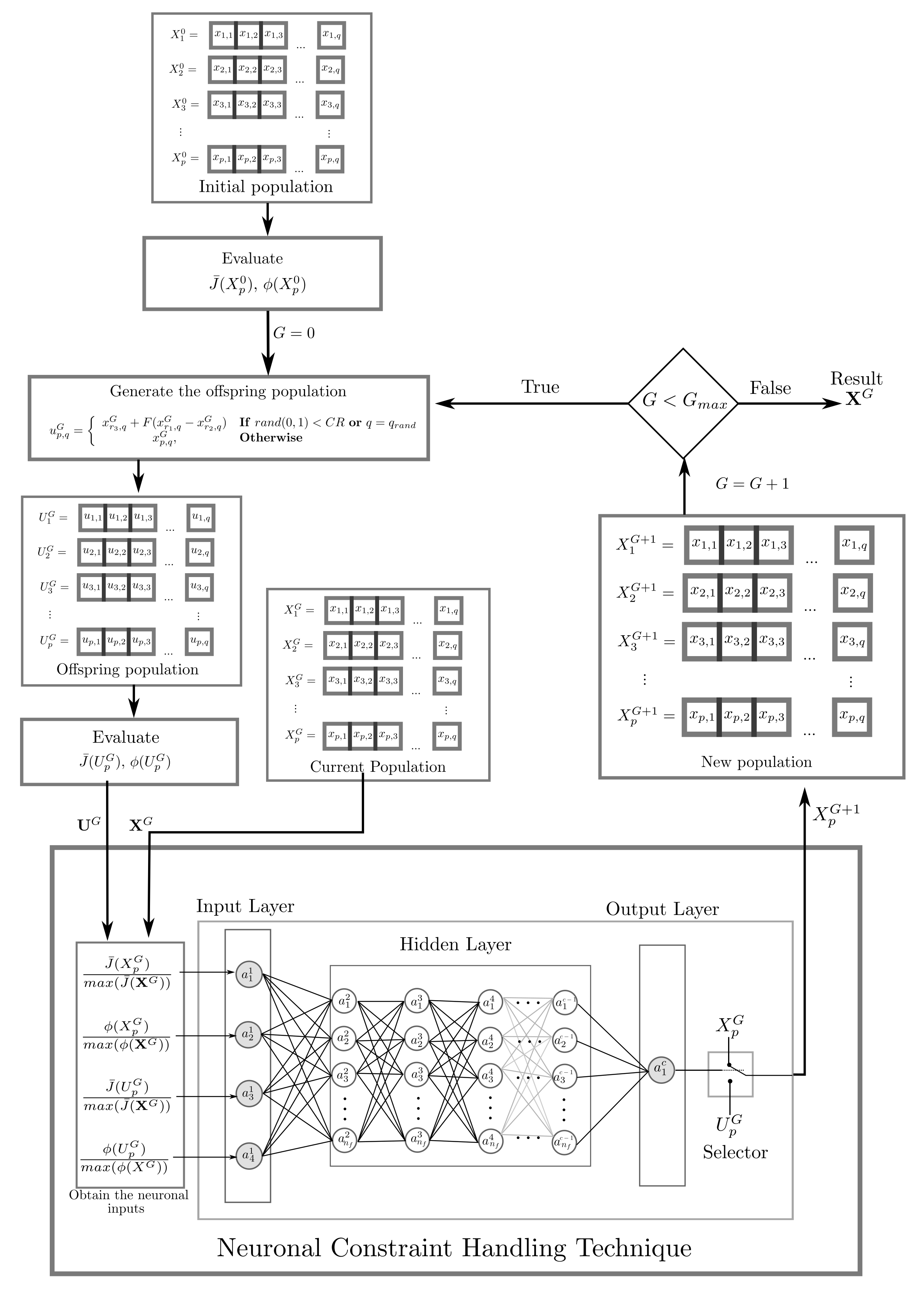
Thirty executions are carried out to evaluate the metaheuristic algorithm performance (DE/RAND/1/BIN, GA, PSO, MUMSA) for each constraint-handling technique (FR, SR, ϵ C, PF, NCH). The acronyms given by the sixteen algorithms are related to the algorithms’ acronym, followed by the constraint-handling technique through a dash. For instance, in the case of algorithms related to the DE/RAND/1/BIN, the acronyms are expressed as R1B-FR, R1B-SR, R1B- ϵ C, and R1B-PF.
The algorithm parameters presented in Table 2, and Table 3 and Table 4 are considered in the executions. Sixty individuals, particles, or chromosomes ( N P = 60 ) and 600,000 objective function evaluations are established as a stop condition for each algorithm.
The results obtained by each algorithm consider the thirty best objective function values obtained through the thirty executions (one value per each execution). This set of values conforms to one sample for the statistical analysis described in this section for a particular algorithm.
In this section, the samples of all algorithms are analyzed by using descriptive statistics, confidence intervals, and inferential statistics.

4.2.1. Descriptive Statistics

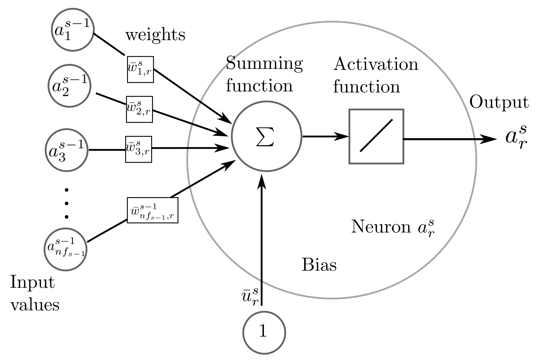
The samples related to thirty executions of algorithms are analyzed by using descriptive statistics metrics, such as the mean, the media, the standard deviation (std), and the maximum (max) and minimum (min) values of the objective function. In addition, the number of Non-Feasible Solutions (NFS) at the end of the optimization process through the thirty executions is also included to know whether the constraint-handling technique shows some issue to leave the infeasible region.
Study case 1:
Table 5 shows the descriptive statistics of samples for study case 1 using trajectory 1 in the synthesis process. The columns are related to the analyzed algorithm, the descriptive statistics metrics, and the NFS for each sample. Boldface indicates the minimum value for each column. According to the results in Table 5, all metaheuristic algorithms find feasible solutions through the thirty executions (see NFS metric). R1B-NCH, R1B-SR, and R1B-PF obtain the three best solutions in that order (see column “min”). R1B-NCH gives the best algorithm performance finding solutions. The obtained solution in R1B-SR and R1B-PF presents an increment of 37.88 % and 41.94 % , respectively, with respect to R1B-NCH (see column “min”). In addition, the mean and minimum results are less in R1B-NCH than other algorithms, and the standard deviation, the median, and maximum values present an average behavior.
Table 6 shows the descriptive statistics of the samples for study case 1 using trajectory 2 in the synthesis process. The columns of such tables contain the same terms explained above. In this analysis, the R1B-NCH algorithm reliability is studied under trajectory changes to be followed by the four–bar linkage mechanism. According to the results in Table 6, all metaheuristic algorithms find feasible solutions (see “NFS” column). MUMSA- ϵ C, R1B-FR, and R1B-NCH obtain the three best solutions in that order. In spite of R1B-NCH presenting the third position, the difference with respect to the MUMSA- ϵ C is minimal at around 2.59 % (see “min” column). Moreover, the R1B-NCH algorithm has the best mean value, indicating the consistency of results through different executions. The standard deviation, the median, the maximum, and minimum values of the objective function have average performance in the R1B-NCH with respect to other algorithms.
Study case 2:
Table 7 shows the descriptive statistics for study case 2 using trajectory 1 in the synthesis process. The columns of such tables contain the same terms explained above. According to the results in Table 7, all metaheuristic algorithms find feasible solutions except for the PSO-FR and R1B-SR algorithm (see “NFS” column). R1B-NCH, MUMSA-FR, and MUMSA- ϵ C obtain the three best solutions (see “min” column). R1B-NCH gives the best algorithm performance finding solutions due to the mean, the median, and the min value of the best objective function being less than other algorithms. The standard deviation and the maximum value of the objective function also present a lower value than the average in the proposal.
Table 8 shows the descriptive statistics for study case 2 using trajectory 2 in the synthesis process. The columns of such tables contain the same terms explained above. In this analysis, the R1B-NCH algorithm reliability is studied under a trajectory change in the cam–linkage mechanism. According to the results in Table 8, all metaheuristic algorithms find feasible solutions except for PSO-FR, R1B-SR, and PSO- ϵ C (see “NFS” column). MUMSA-FR, R1B-NCH, and MUMSA-SR obtain the three best solutions in that order. The R1B-NCH presents a very slight increment of around 0.68 % with respect to the obtained result given in MUMSA-FR (see “min” column). The R1B-NCH also obtains the best values in the mean, the standard deviation, the median, and the maximum value of the objective function.
It is observed in Table 5, Table 6, Table 7 and Table 8 that the R1B-NCH presents an outstanding mean performance (see “mean” columns) in the search for solutions through study cases in spite of presenting changes in the optimization problems (rehabilitation trajectories) where the algorithm setting and the NCH technique were tuned and trained, respectively.
However, descriptive statistics cannot estimate the best algorithm behaviors for future executions. Therefore, the analysis of results by 95 % confidence intervals and inferential statistics [56] is carried out in the next section.

4.2.2. Confidence Intervals and Inferential Statistics

This section confirms the best algorithm behavior to solve each study case considered in this work. The best algorithm behavior is obtained by analyzing the sample (thirty best values of the objective function) obtained in each algorithm execution by 95 % confidence intervals [61] and using the non-parametric Friedman test [56].
The 95 % Confidence Interval (CI) [61] is a range of values for a selected sample of a study, where, with a 95 % confidence, the interval contains the population’s true mean. Therefore, the confidence interval values closest to zero indicate the most promising algorithm due to the high probability that the mean behavior of the algorithm is inside such interval. Moreover, in what follows, for each study case, the use of inferential statistics through the Friedman test of the algorithm samples with the best CI will confirm the algorithm performance.
Study case 1:
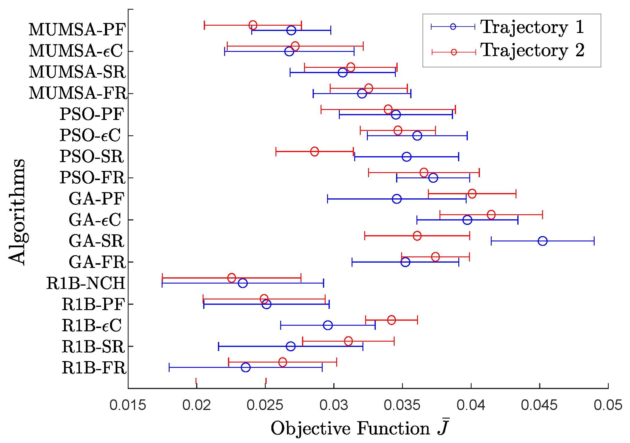
Table 9 shows the confidence interval values obtained by each algorithm for study case 1 using both trajectories, and Figure 7 shows its graphical representation. It is observed that the R1B-NCH, the R1B-PF, and the MUMSA-PF have confidence intervals closer to zero (to the left) for trajectory 1. The R1B-NCH presents the confidence interval lower limit value closest to zero, and its confidence interval upper limit does not exceed the MUMSA-PF confidence interval upper limit. The results using trajectory 2 show that R1B-FR, R1B-PF, and R1B-NCH have confidence intervals closer to zero. The R1B-NCH presents the confidence interval lower limit value closest to zero, and the upper limit does not exceed the confidence interval upper limit of R1B-FR.
The 95 % -confidence Friedman test is carried out in those three outstanding algorithms per each trajectory, i.e., in R1B-NCH, R1B-PF, and MUMSA-PF for trajectory 1; and, in R1B-FR, R1B-PF, and R1B-NCH for trajectory 2. According to the Friedman test in those groups of three algorithms, there is no statistically significant difference in the comparisons because the returned p-value is greater than 0.05 . It is also confirmed in the multiple comparisons with the Bonferroni post-hoc error correction method of the Friedman test given in Table 10 that the associated p-value is greater than 0.05 , indicating the no confirmation of the superiority of one algorithm in the comparison. In this paper, a tie is declared in the comparison when that situation occurs. Thus, in all comparisons presented in Table 10, the algorithms draw.
In the mechanism synthesis problem, it is common to obtain the optimal solution by setting different (usually thirty) executions to the same problem [47]. However, there may be significant differences among the best solutions obtained through different executions, and the most promising solution obtained by the optimizer in the mechanism synthesis problem is given through the best solution among executions [62].
Then, to know whether the proposed R1B-NCH empirically presents a high probability of finding the best results in the kinematic synthesis problem for lower limb rehabilitation, the following is defined: As the confidence interval indicates whether these executions are repeated in several tests, the proportion of calculated 95 % confidence intervals that is included the population’s true mean value would tend toward 95 % ; then, the confidence interval closest to zero will indicate the population’s true mean value is closer to the reduction of the objective function, and, hence, it is assumed that this interval presents a high probability of granting the best solution (minimum value) through thirty executions of the algorithm (executions commonly used for finding the best solution in the mechanism synthesis problem).
In order to verify the previous assumption, the other four sets of thirty executions are performed for the two groups of three algorithms (R1B-NCH, R1B-PF, and MUMSA-PF for trajectory 1; and R1B-FR, R1B-PF, and R1B-NCH for trajectory 2). In Table 11, the minimum values from the thirty executions per set are displayed. It is observed that, in each column related to the set of data for the corresponding trajectories, the minimum value, marked in boldface, is obtained by the proposed R1B-NCH.
According to this analysis for study case 1, it is observed that the R1B-NCH algorithm presents a high probability to find the best solution through thirty executions of the algorithm in the mechanism synthesis problem for lower limb rehabilitation.
Study case 2:
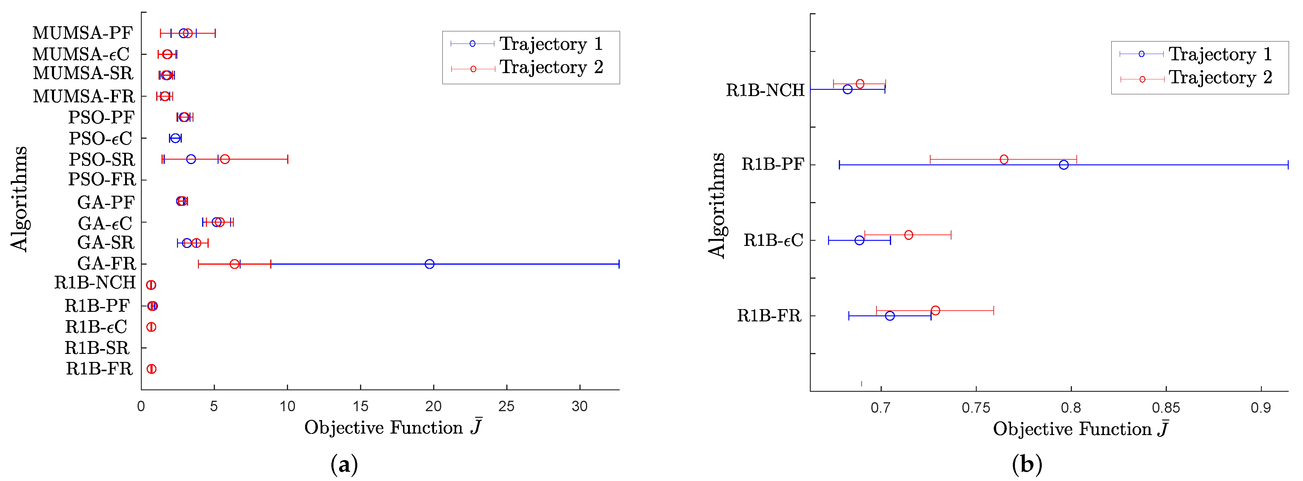
Table 12 shows the confidence intervals obtained by each algorithm for study case 2 using both trajectories. Figure 8a shows the graphical representation of the confidence interval, and Figure 8b shows the close-up view of the confidence intervals closer to zero. According to the results for both trajectories, R1B-FR, R1B- ϵ C, and R1B-NCH have confidence intervals closer to zero, where R1B-NCH presents the confidence interval lower limit value closest to zero and its upper limit does not exceed the R1B- ϵ C confidence interval upper limit.
The 95 % -confidence Friedman test is performed in those three outstanding algorithms, i.e., in R1B-FR, R1B- ϵ C, and R1B-NCH for both trajectories. According to the Friedman test in those groups of three algorithms, there exist a statistically significant difference among them in both trajectories because the p-value associated is less than the proposed significance level. Hence, to determine if one algorithm outperforms the other, inferential statistics given by the Friedman test for multiple comparisons with the Bonferroni post-hoc error correction method is carried out for finding the accurate pairwise comparisons. In Table 13, such tests are given, and in boldface, the winner in the comparison is highlighted. According to the number of wins, the results indicate that R1B-NCH is the most promising optimizer in the optimal synthesis for the study case 2 in both trajectories because it wins in all comparisons.
In order to empirically confirm the superiority of the proposed R1B-NCH, to obtain the optimal solution by setting different (usually thirty) executions to the same problem, other four sets of thirty executions are performed for the two groups of three algorithms (R1B-FR, R1B- ϵ C, and R1B-NCH for both trajectories). In Table 14, the minimum values from the thirty executions per set are displayed. It is observed that, in each column, the minimum value, marked in boldface, is given by the expected algorithm (based on Table 13), i.e., the proposed R1B-NCH. Note that these boldface values cannot be reached by the other algorithms (R1B-FR and R1B- ϵ C), confirming the statistical analysis presented above.

4.2.3. Overall Evaluation of the Proposed NCH through Study Cases

The overall evaluation of the most promising algorithms given in Section 4.2.2 is discussed next.
In the first study case and according to Table 10, the most promising algorithms considering both trajectories are: R1B-NCH, R1B-PF, MUMSA-PF, and R1B-FR. In that case, all algorithms draw with each other. Thus, each algorithm presents two draws. In the second study case and according to Table 13, the most promising algorithms are: R1B-NCH, R1B-EC, and R1B-FR. In such a case, the R1B-NCH wins four times, and the R1B-EC wins one time. With this information, a summary of the number of wins and draws for both study cases, and trajectories are presented in Table 15. According to this table, the overall evaluation of the most promising algorithms is analyzed, and it is confirmed that the most promising one is the proposed R1B-NCH because it wins and draws four times. The next best behaviors of the algorithms to solve the synthesis problem are related to R1B-PF and R1B-FR in that order.
Then, the NCH technique increases the exploration and exploitation capabilities in the ED/RAND/1/BIN algorithm to solve the considered mechanism synthesis problems. The obtained solution (mechanism) could improve the lower limb rehabilitation machine.
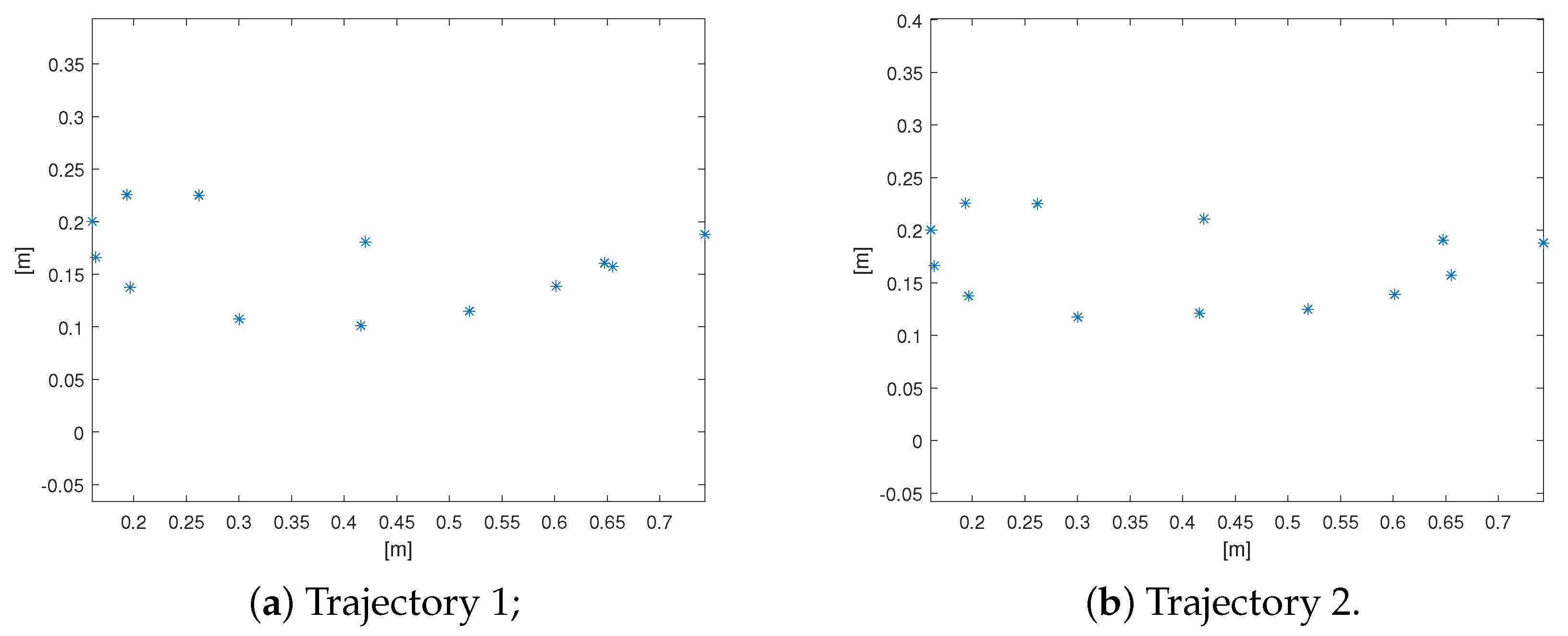
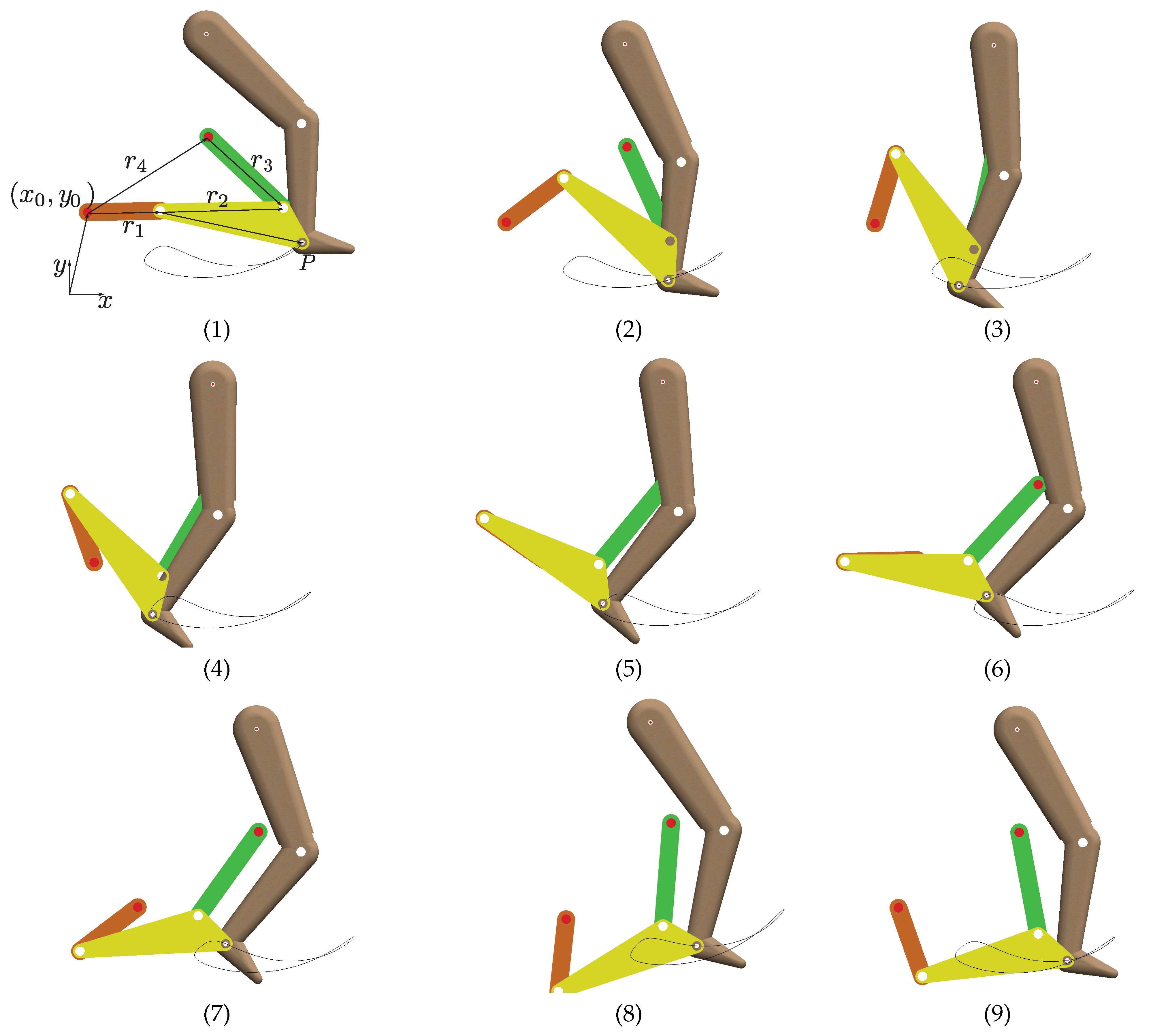
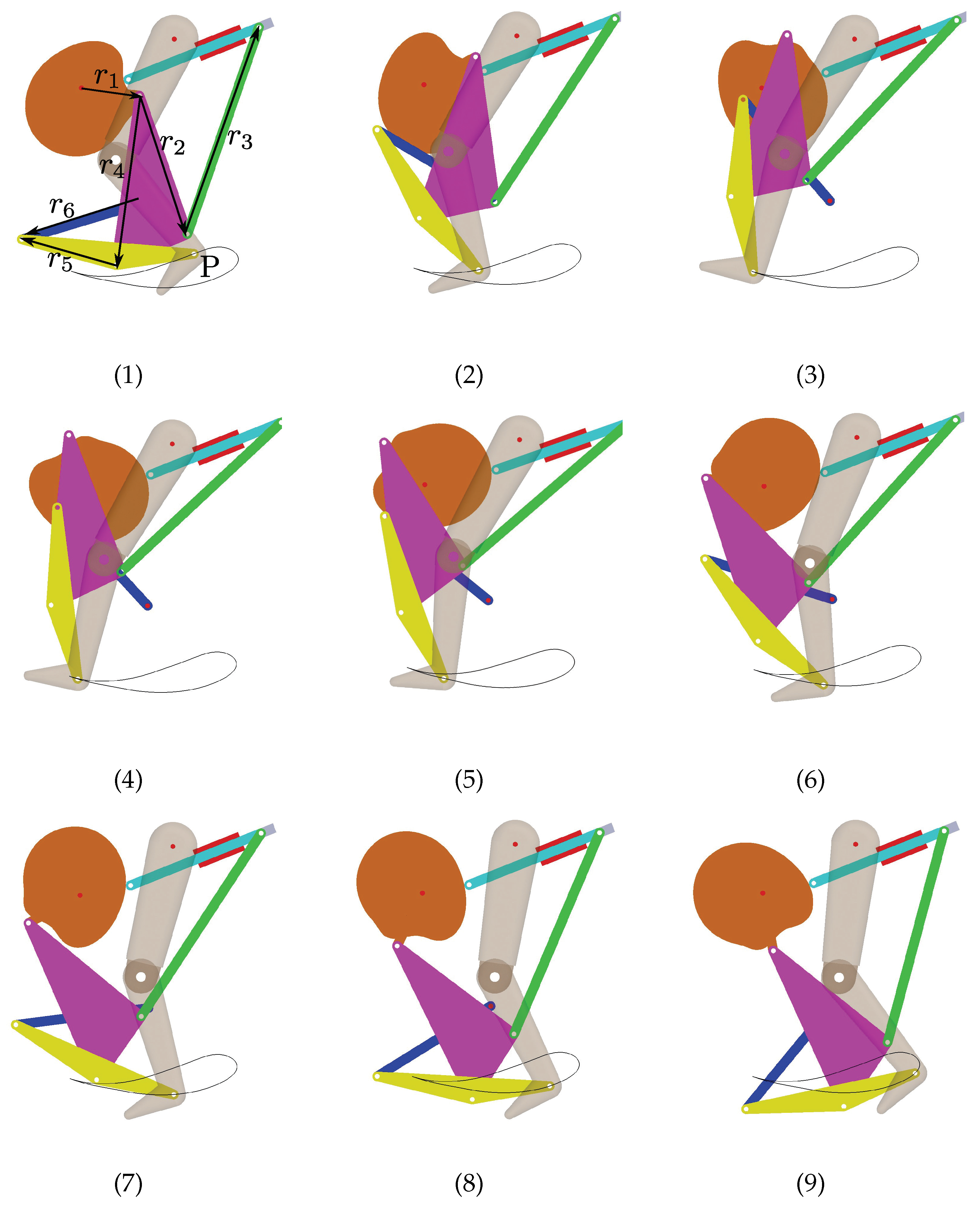
Finally, the best solutions obtained by the R1B-NCH algorithm for each study case are displayed in Table 16 and Table 17. In order to validate the obtained mechanism for rehabilitation purposes, the Computer-Aided Design (CAD) of the mechanism in different phases of the crank movement is shown in Figure 9 and 
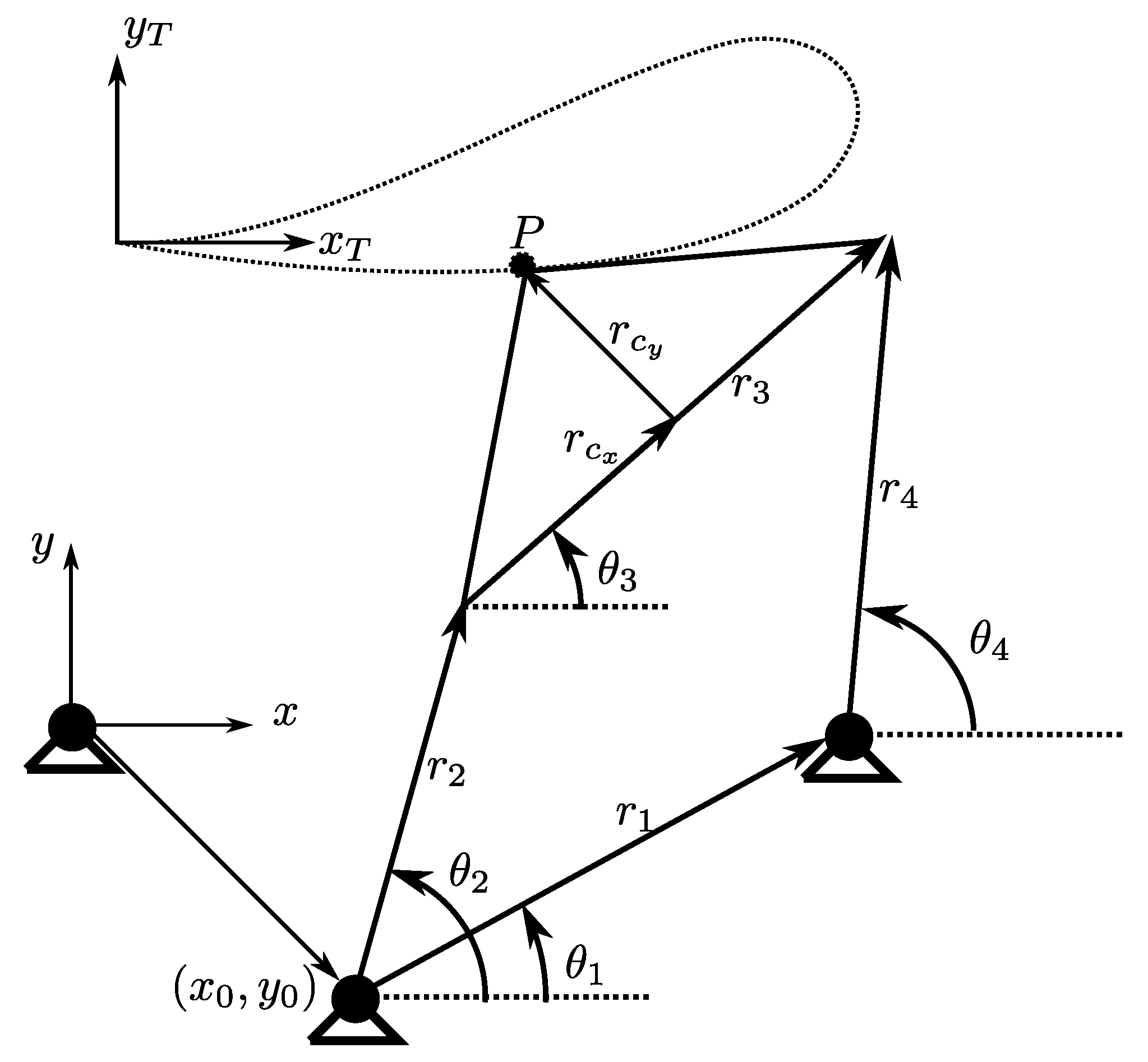
Figure 10. Through the figure sequences given by the number 1 to the sequence number 9, it is observed that the coupler point of the mechanism in both figures can provide the proposed rehabilitation routine showing in a continuous line. Furthermore, if we fixed the human ankle joint in the coupler point of the mechanism, the mechanism can reproduce the natural movement of the leg, as is shown in those figures.

5. Conclusions

In this work, the Neuronal Constraint-Handling (NCH) technique is proposed and included in the differential evolution variant ED/RAND/1/BIN algorithm. The proposal is validated in the solution of synthesis problems of the four–bar and cam–linkage mechanisms (two study cases) for developing lower-limb rehabilitation routines.
The constraint-handling techniques FR, SR, ϵ C, and PF are included in the metaheuristic algorithms DE/RAND/1/BIN, GA, PSO, and MUMSA for comparative purposes.
The NCH performance is fairly and meaningfully compared with sixteen metaheuristic algorithms using the irace package for both the algorithm settings and neuronal network training, and the statistical analysis for the confirmation of the overall performance.
The statistical results confirm that the proposed R1B-NCH presents the best overall performance in spite of using different trajectories than were used to tune the algorithms and train the NCH technique. Furthermore, the results indicate that the NCH technique balances the exploration and exploitation capabilities in the ED/RAND/1/BIN algorithm to solve the considered mechanism synthesis problems and thus obtains better design solutions.
Future work involves the use and the comparative study of other neuronal network architecture such as recurrent neural networks and symmetrically connected neural networks as constraint handling techniques. Recent authors’ work indicates that the use of the relative angle method in the development of the kinematic motion in the synthesis problem of mechanism indirectly increases the exploration capability of the algorithms, i.e., the statement of the optimization problem highly influences in the optimizer. The use of NCH techniques with the relative angle method could benefit the search and improve the obtained results. Another research direction involves using the NCH technique in multi-objective search approaches for the mechanism synthesis problems in rehabilitation routines.

Author Contributions

Conceptualization, J.S.M.-R. and M.G.V.-C.; Data curation, J.S.M.-R.; Formal analysis, J.S.M.-R.; Funding acquisition, M.G.V.-C. and L.G.C.-R.; Investigation, J.S.M.-R. and M.G.V.-C.; Methodology, J.S.M.-R. and M.G.V.-C.; Project administration, M.G.V.-C.; Resources, L.G.C.-R.; Software, J.S.M.-R.; Supervision, M.G.V.-C.; Validation, J.S.M.-R., M.G.V.-C. and L.E.V.-S.; Visualization, J.S.M.-R. and L.E.V.-S.; Writing—original draft, J.S.M.-R. and M.G.V.-C.; Writing—review and editing, J.S.M.-R. and M.G.V.-C. All authors have read and agreed to the published version of the manuscript.

Funding

This research was funded by Secretaría de Investigación y Posgrado del Instituto Politécnico Nacional (SIP-IPN) Grant Nos. 20180196, 20220255, 20181312, 20196226, 20201406, and 20221407.

Institutional Review Board Statement

Not applicable.

Informed Consent Statement

Not applicable.

Data Availability Statement

The data presented in this study are available on request from the corresponding author.

Acknowledgments

The authors acknowledge support from the Secretaría de Investigación y Posgrado (SIP) and the Comisión de Operación y Fomento de Actividades Académicas (COFAA) of the Instituto Politécnico Nacional (IPN). The first and fourth authors acknowledge support from the Mexican Consejo Nacional de Ciencia y Tecnología (CONACyT) through a scholarship to pursue graduate studies at CIDETEC-UPIITA-IPN.

Conflicts of Interest

The authors declare no conflict of interest.

Abbreviations and Nomenclature

Abbreviations

NCHNeuronal Constraint-Handling
DEDifferential Evolution
DE/RAND/1/BINDE variant with random mutation an binomial crossover
SQPSequential Quadratic Programming
GAGenetic Algorithm
PSOParticle Swarm Optimization
MUMSAMalaga University Mechanism Synthesis Algorithm
POEMAPareto Optimum Evolutionary multi-objective Algorithm
GA-FLGA–Fuzzy Logic
AGAnt-Gradient
CSCuckoo Search
ICAImperialist Competitive Algorithm
TLBOTeaching-Learning-Based Optimization
HLIDEHybrid Lagrange Interpolation DE
CMDECombined-Mutation DE
CHTConstraint-Handling Techniques

Nomenclature

J ¯ Weighted objective function
J i i-th objective function
xDesign variable vector
g j j-th inequality constraint
h k k-th equality constraint
x m i n & x m a x Upper and lower design variable vector bounds
X G Population of individuals in a G generation
X p G p-th individual in the X G population
U G Offspring individuals in a G generation
ϕ Constraint distance
f ( μ ) Sigmoid function
a r s r-th neuron in s-th layer in NCH technique
w ^ t , r s t-th wight for a r s neuron
a r s r-th bias in s-th layer for a r s neuron
w i i-th weight in the objective function
[ x ¯ p i , y ¯ p i ] Desired path points
[ x p i , y p i ] Mechanism path points
r i i-th length link
θ 2 i i-th crank angle
[ x 0 , y 0 ] Ground link origin
[ r c x , r c y ] Lengths in the coupler link
β , γ & η Link angles
eSlider displacement
α Slider angular position
R 0 Cam base radius
Θ r e f Normalization angle parameter
R r e f Normalization radius parameter
d i j Distance between i to j point
C R Crossover factor
F m i n & F m a x Maximum and minimum scale factor limit
M R Mutation rate
P f Probabilistic factor in SR
c p Control the relaxation of constraints
T c Maximum iterations to relax constraints
R G Number of attempts to improve a solution
P g Probabilistic factor to improve a solution

Appendix A. Trajectories for Rehabilitation in the Study Cases

Table A1. Cartesian coordinates of the precision points for both trajectories in study case 1.
Trajectory 1Trajectory 2
x [m]y [m]x [m]y [m]
0.74290.1880.74290.188
0.65510.15730.65510.1573
0.60140.13880.60140.1388
0.51890.11490.51890.1249
0.41590.10120.41590.1212
0.30010.10740.30010.1174
0.19640.13750.19640.1375
0.16390.16620.16390.1662
0.16050.20030.16050.2003
0.19340.22560.19340.2256
0.26190.22510.26190.2251
0.42010.18080.42010.2108
0.64740.16070.64740.1907
0.74290.1880.74290.188
Table A2. Cartesian coordinates of the precision points for trajectory 1 in study case 2.
x [mm]y [mm]x [mm]y [mm]x [mm]y [mm]
−315.8706−725.914102.286−784.1517249.9019−624.0724
−305.426−729.4993113.9412−782.7289232.1635−626.9287
−295.562−732.633126.2456−780.9599214.5033−631.2082
−284.9638−735.7146137.8298−779.0587195.4565−636.575
−272.9513−738.8459150.0497−776.7977175.5689−643.126
−259.5651−742.091162.2326−774.345154.0295−650.5493
−245.4816−745.2649175.691−771.2814132.9875−658.2092
−230.7078−748.3559188.404−768.0873110.6898−666.7843
−217.2474−750.9006201.7067−764.441988.04307−675.2332
−201.8657−754.024214.2527−760.680662.68539−684.4142
−188.5033−756.6797228.0001−756.168437.99372−693.0726
−173.8345−759.6436240.3332−751.800613.98859−701.2471
−161.1907−762.2906253.8222−746.6116−13.02161−709.5296
−147.8624−764.9876265.2127−741.7514−38.76389−716.7951
−134.5299−767.7142277.7069−736.0049−65.7052−723.5015
−122.5271−770.2517289.3726−730.1277−93.18724−729.2118
−111.1662−772.6216300.7921−723.7715−119.8744−733.994
−98.40761−774.9819310.6746−717.4391−147.5638−737.2401
−86.97769−777.2058320.2523−710.5785−172.2932−739.7084
−74.81197−779.1819328.2496−703.7132−197.8191−740.6221
−63.29198−781.0032335.1887−696.3953−222.7483−740.2338
−51.73248−782.6248339.9644−689.448−244.9169−738.7976
−40.13729−784.046343.6156−681.9446−266.9157−735.9746
−28.51026−785.2659345.5832−674.264−284.0916−733.2587
−16.16956−786.2028346.533−666.2336−299.6447−729.774
−4.491148−787.0124344.1531−659.0253−313.0036−726.1448
7.891441−787.5247340.7879−651.3812−321.6559−723.6518
19.6055−787.922335.573−644.3309−328.838−721.1686
30.63857−788.0627327.8983−637.91−332.1062−720.0498
43.05355−787.9534318.5382−632.043−332.155−720.179
54.77622−787.6019307.4652−627.8585−329.6154−721.2705
67.19192−787.0725295.572−624.2872−323.2063−723.8421
78.90697−786.3287281.0296−622.9766−316.7307−726.2375
91.2885−785.2526266.4392−622.3635
Table A3. Cartesian coordiantes of the precision points for trajectory 2 in study case 2.
x [mm]y [mm]x [mm]y [mm]x [mm]y [mm]
−315.8706−725.914102.286−777.1517249.9019−624.0724
−305.426−729.4993113.9412−776.7289232.1635−626.9287
−295.562−732.633126.2456−776.9599214.5033−631.2082
−284.9638−735.7146137.8298−776.0587195.4565−636.575
−272.9513−738.8459150.0497−774.7977175.5689−643.126
−259.5651−742.091162.2326−773.345154.0295−650.5493
−245.4816−745.2649175.691−771.2814132.9875−658.2092
−230.7078−748.3559188.404−768.0873110.6898−666.7843
−217.2474−750.9006201.7067−764.441988.04307−675.2332
−201.8657−754.024214.2527−760.680662.68539−680.4142
−188.5033−756.6797228.0001−756.168437.99372−685.0726
−173.8345−759.6436240.3332−751.800613.98859−687.2471
−161.1907−762.2906253.8222−746.6116−13.02161−692.5296
−147.8624−764.9876265.2127−741.7514−38.76389−697.7951
−134.5299−767.7142277.7069−736.0049−65.7052−701.5015
−122.5271−770.2517289.3726−730.1277−93.18724−702.2118
−111.1662−772.6216300.7921−723.7715−119.8744−701.994
−98.40761−774.9819310.6746−717.4391−147.5638−703.2401
−86.97769−777.2058320.2523−710.5785−172.2932−703.7084
−74.81197−777.1819328.2496−703.7132−197.8191−704.6221
−63.29198−777.0032335.1887−696.3953−222.7483−702.2338
−51.73248−776.6248339.9644−689.448−244.9169−700.7976
−40.13729−777.046343.6156−681.9446−266.9157−697.9746
−28.51026−778.2659345.5832−674.264−284.0916−698.2587
−16.16956−778.2028346.533−666.2336−299.6447−699.774
−4.491148−778.0124344.1531−659.0253−313.0036−701.1448
7.891441−778.5247340.7879−651.3812−321.6559−703.6518
19.6055−777.922335.573−644.3309−328.838−705.1686
30.63857−778.0627327.8983−637.91−332.1062−708.0498
43.05355−777.9534318.5382−632.043−332.155−710.179
54.77622−777.6019307.4652−627.8585−329.6154−713.2705
67.19192−777.0725295.572−624.2872−323.2063−718.8421
78.90697−777.3287281.0296−622.9766−316.7307−721.2375
91.2885−777.2526266.4392−622.3635

References

  1. Maciejasz, P.; Eschweiler, J.; Gerlach-Hahn, K.; Jansen-Troy, A.; Leonhardt, S. A survey on robotic devices for upper limb rehabilitation. J. Neuroeng. Rehabil. 2014, 11, 3. [Google Scholar] [CrossRef] [Green Version]
  2. Díaz, I.; Gil, J.J.; Sánchez, E. Lower-limb robotic rehabilitation: Literature review and challenges. J. Robot. 2011, 2011, 759764. [Google Scholar] [CrossRef]
  3. Muñoz-Reina, J.S.; Villarreal-Cervantes, M.G.; Corona-Ramírez, L.G. Integrated design of a lower limb rehabilitation mechanism using differential evolution. Comput. Electr. Eng. 2021, 92, 107103. [Google Scholar] [CrossRef]
  4. Norton, R.L. Design of Machinery: An Introduction to the Synthesis and Analysis of Mechanisms and Machines; McGraw-Hill/Higher Education: New York, NY, USA, 2008. [Google Scholar]
  5. Cabrera, J.; Simon, A.; Prado, M. Optimal synthesis of mechanisms with genetic algorithms. Mech. Mach. Theory 2002, 37, 1165–1177. [Google Scholar] [CrossRef] [Green Version]
  6. Bulatović, R.R.; Đorđević, S.R.; Đorđević, V.S. Cuckoo Search algorithm: A metaheuristic approach to solving the problem of optimum synthesis of a six-bar double dwell linkage. Mech. Mach. Theory 2013, 61, 1–13. [Google Scholar] [CrossRef]
  7. Calva-Yáñez, M.B.; Niño-Suarez, P.A.; Portilla-Flores, E.A.; Aponte-Rodríguez, J.A.; Santiago-Valentn, E. Reconfigurable mechanical system design for tracking an ankle trajectory using an evolutionary optimization algorithm. IEEE Access 2017, 5, 5480–5493. [Google Scholar] [CrossRef]
  8. Bulatović, R.R.; Miodragović, G.; Bošković, M.S. Modified Krill Herd (MKH) algorithm and its application in dimensional synthesis of a four–bar linkage. Mech. Mach. Theory 2016, 95, 1–21. [Google Scholar] [CrossRef]
  9. Rao, S.S. Engineering Optimization-Theory and Practice, 4th ed.; Wiley: Hoboken, NJ, USA, 2009. [Google Scholar]
  10. Ávila Hernández, P.; Cuenca-Jiménez, F. Design and synthesis of a 2 DOF 9-bar spatial mechanism for a prosthetic thumb. Mech. Mach. Theory 2018, 121, 697–717. [Google Scholar] [CrossRef]
  11. Ji, Z.; Manna, Y. Synthesis of a pattern generation mechanism for gait rehabilitation. J. Med. Devices 2008, 2, 1–8. [Google Scholar] [CrossRef]
  12. Wang, H.; Wu, J.; Wang, Y.; Ren, L.; Zhang, D.; Lu, H. Research on the lower limb gait rehabilitation. In Proceedings of the 2014 IEEE International Conference on Mechatronics and Automation, Tianjin, China, 3–6 August 2014; pp. 1243–1247. [Google Scholar]
  13. Tsuge, B.Y.; McCarthy, J.M. Synthesis of a 10-bar linkage to guide the gait cycle of the human leg. In Proceedings of the ASME 2015 International Design Engineering Technical Conferences and Computers and Information in Engineering Conference; American Society of Mechanical Engineers Digital Collection: New York, NY, USA, 2015; pp. 1–7. [Google Scholar]
  14. Tsuge, B.Y.; Plecnik, M.M.; Michael McCarthy, J. Homotopy directed optimization to design a six-bar linkage for a lower limb with a natural ankle trajectory. J. Mech. Robot. 2016, 8, 061009. [Google Scholar] [CrossRef] [Green Version]
  15. Conway, B.A. A survey of methods available for the numerical optimization of continuous dynamic systems. J. Optim. Theory Appl. 2012, 152, 271–306. [Google Scholar] [CrossRef]
  16. Holland, J.H. Adaptation in Natural and Artificial Systems: An Introductory Analysis with Applications to Biology, Control, and Artificial Intelligence; MIT Press: Cambridge, MA, USA, 1992. [Google Scholar]
  17. Cabrera, J.; Ortiz, A.; Nadal, F.; Castillo, J. An evolutionary algorithm for path synthesis of mechanisms. Mech. Mach. Theory 2011, 46, 127–141. [Google Scholar] [CrossRef]
  18. Kennedy, J.; Eberhart, R. Particle swarm optimization. In Proceedings of the ICNN’95-International Conference on Neural Networks, Perth, WA, Australia, 27 November–1 December 1995; Volume 4, pp. 1942–1948. [Google Scholar]
  19. Yang, X.S. Harmony Search as a Metaheuristic Algorithm. In Music-Inspired Harmony Search Algorithm: Theory and Applications; Geem, Z.W., Ed.; Springer: Berlin/Heidelberg, Germany, 2009; pp. 1–14. [Google Scholar]
  20. Hamed, M.M.; Abdy, H.; Zahiri, S.H. IPO: An inclined planes system optimization algorithm. Comput. Inform. 2016, 35, 222–240. [Google Scholar]
  21. Bataller, A.; Cabrera, J.; Clavijo, M.; Castillo, J. Evolutionary synthesis of mechanisms applied to the design of an exoskeleton for finger rehabilitation. Mech. Mach. Theory 2016, 105, 31–43. [Google Scholar] [CrossRef]
  22. Shao, Y.; Xiang, Z.; Liu, H.; Li, L. Conceptual design and dimensional synthesis of cam–linkage mechanisms for gait rehabilitation. Mech. Mach. Theory 2016, 104, 31–42. [Google Scholar] [CrossRef]
  23. Singh, R.; Chaudhary, H.; Singh, A.K. A novel gait-based synthesis procedure for the design of 4-bar exoskeleton with natural trajectories. J. Orthop. Transl. 2018, 12, 6–15. [Google Scholar] [CrossRef]
  24. Coello, C.A.C. Theoretical and numerical constraint-handling techniques used with evolutionary algorithms: A survey of the state of the art. Comput. Methods Appl. Mech. Eng. 2002, 191, 1245–1287. [Google Scholar] [CrossRef]
  25. Cervantes-Culebro, H.; Cruz-Villar, C.A.; Peñaloza, M.G.M.; Mezura-Montes, E. Constraint-handling techniques for the concurrent design of a five-bar parallel robot. IEEE Access 2017, 5, 23010–23021. [Google Scholar] [CrossRef]
  26. Miranda-Varela, M.E.; Mezura-Montes, E. Constraint-handling techniques in surrogate-assisted evolutionary optimization. An empirical study. Appl. Soft Comput. 2018, 73, 215–229. [Google Scholar] [CrossRef]
  27. Mezura-Montes, E.; Coello Coello, C.A. Constraint-handling in nature-inspired numerical optimization: Past, present and future. Swarm Evol. Comput. 2011, 1, 173–194. [Google Scholar] [CrossRef]
  28. He, X.S.; Fan, Q.W.; Karamanoglu, M.; Yang, X.S. Comparison of Constraint-Handling Techniques for Metaheuristic Optimization. In Proceedings of the Computational Science–ICCS 2019; Rodrigues, J.M.F., Cardoso, P.J.S., Monteiro, J., Lam, R., Krzhizhanovskaya, V.V., Lees, M.H., Dongarra, J.J., Sloot, P.M., Eds.; Springer International Publishing: Cham, Switzerland, 2019; pp. 357–366. [Google Scholar]
  29. Muñoz-Reina, J.S.; Villarreal-Cervantes, M.G.; Corona-Ramírez, L.G. Empirical Study of Constraint-Handling Techniques in the Optimal Synthesis of Mechanisms for Rehabilitation. Appl. Sci. 2021, 11, 8739. [Google Scholar] [CrossRef]
  30. Smith, A.E.; Coit, D.W.; Baeck, T.; Fogel, D.; Michalewicz, Z. Penalty functions. Handb. Evol. Comput. 1997, 97, 1–12. [Google Scholar]
  31. Shiakolas, P.; Koladiya, D.; Kebrle, J. On the optimum synthesis of four–bar linkages using differential evolution and the geometric centroid of precision positions. Inverse Probl. Eng. 2002, 10, 485–502. [Google Scholar] [CrossRef]
  32. Bulatović, R.R.; Dordević, S.R. On the optimum synthesis of a four–bar linkage using differential evolution and method of variable controlled deviations. Mech. Mach. Theory 2009, 44, 235–246. [Google Scholar] [CrossRef]
  33. Shiakolas, P.; Koladiya, D.; Kebrle, J. On the optimum synthesis of six-bar linkages using differential evolution and the geometric centroid of precision positions technique. Mech. Mach. Theory 2005, 40, 319–335. [Google Scholar] [CrossRef]
  34. Laribi, M.; Mlika, A.; Romdhane, L.; Zeghloul, S. A combined genetic algorithm–fuzzy logic method (GA–FL) in mechanisms synthesis. Mech. Mach. Theory 2004, 39, 717–735. [Google Scholar] [CrossRef]
  35. Acharyya, S.; Mandal, M. Performance of EAs for four–bar linkage synthesis. Mech. Mach. Theory 2009, 44, 1784–1794. [Google Scholar] [CrossRef]
  36. Smaili, A.; Diab, N. Optimum synthesis of hybrid-task mechanisms using ant-gradient search method. Mech. Mach. Theory 2007, 42, 115–130. [Google Scholar] [CrossRef]
  37. Ebrahimi, S.; Payvandy, P. Efficient constrained synthesis of path generating four–bar mechanisms based on the heuristic optimization algorithms. Mech. Mach. Theory 2015, 85, 189–204. [Google Scholar] [CrossRef]
  38. Zhang, K.; Huang, Q.; Zhang, Y.; Song, J.; Shi, J. Hybrid Lagrange interpolation differential evolution algorithm for path synthesis. Mech. Mach. Theory 2019, 134, 512–540. [Google Scholar] [CrossRef]
  39. Sancibrian, R.; Sedano, A.; Sarabia, E.G.; Blanco, J.M. Hybridizing differential evolution and local search optimization for dimensional synthesis of linkages. Mech. Mach. Theory 2019, 140, 389–412. [Google Scholar] [CrossRef]
  40. Deb, K. An efficient constraint handling method for genetic algorithms. Comput. Methods Appl. Mech. Eng. 2000, 186, 311–338. [Google Scholar] [CrossRef]
  41. Cabrera, J.; Nadal, F.; Munoz, J.; Simon, A. multi-objective constrained optimal synthesis of planar mechanisms using a new evolutionary algorithm. Mech. Mach. Theory 2007, 42, 791–806. [Google Scholar] [CrossRef]
  42. Runarsson, T.P.; Yao, X. Stochastic ranking for constrained evolutionary optimization. IEEE Trans. Evol. Comput. 2000, 4, 284–294. [Google Scholar] [CrossRef] [Green Version]
  43. Takahama, T.; Sakai, S.; Iwane, N. Constrained optimization by the ε constrained hybrid algorithm of particle swarm optimization and genetic algorithm. In Proceedings of the Australasian Joint Conference on Artificial Intelligence; Springer: Berlin/Heidelberg, Germany, 2005; pp. 389–400. [Google Scholar]
  44. Huang, Q.; Yu, Y.; Zhang, K.; Li, S.; Lu, H.; Li, J.; Zhang, A.; Mei, T. Optimal synthesis of mechanisms using repellency evolutionary algorithm. Knowl.-Based Syst. 2022, 239, 107928. [Google Scholar] [CrossRef]
  45. Lin, W.Y. A GA–DE hybrid evolutionary algorithm for path synthesis of four–bar linkage. Mech. Mach. Theory 2010, 45, 1096–1107. [Google Scholar] [CrossRef]
  46. Singh, R.; Chaudhary, H.; Singh, A.K. Defect-free optimal synthesis of crank-rocker linkage using nature-inspired optimization algorithms. Mech. Mach. Theory 2017, 116, 105–122. [Google Scholar] [CrossRef]
  47. Valencia-Segura, L.E.; Villarreal-Cervantes, M.G.; Corona-Ramírez, L.G.; Cuenca-Jiménez, F.; Castro-Medina, R. Optimum synthesis of four–bar mechanism by using relative angle method: A comparative performance study. IEEE Access 2021, 9, 132990–133010. [Google Scholar] [CrossRef]
  48. Lin, W.Y.; Hsiao, K.M. Cuckoo search and teaching–learning-based optimization algorithms for optimum synthesis of path-generating four–bar mechanisms. J. Chin. Inst. Eng. 2017, 40, 66–74. [Google Scholar] [CrossRef]
  49. Rafiq, M.; Bugmann, G.; Easterbrook, D. Neural network design for engineering applications. Comput. Struct. 2001, 79, 1541–1552. [Google Scholar] [CrossRef]
  50. Kiranyaz, S.; Avci, O.; Abdeljaber, O.; Ince, T.; Gabbouj, M.; Inman, D.J. 1D convolutional neural networks and applications: A survey. Mech. Syst. Signal Process. 2021, 151, 107398. [Google Scholar] [CrossRef]
  51. Chua, L.O.; Yang, L. Cellular neural networks: Applications. IEEE Trans. Circuits Syst. 1988, 35, 1273–1290. [Google Scholar] [CrossRef]
  52. Widrow, B.; Rumelhart, D.E.; Lehr, M.A. Neural networks: Applications in industry, business and science. Commun. ACM 1994, 37, 93–106. [Google Scholar] [CrossRef]
  53. Kazikova, A.; Pluhacek, M.; Senkerik, R. Why tuning the control parameters of metaheuristic algorithms is so important for fair comparison? Mendel 2020, 26, 9–16. [Google Scholar] [CrossRef]
  54. Huang, C.; Li, Y.; Yao, X. A Survey of Automatic Parameter Tuning Methods for Metaheuristics. IEEE Trans. Evol. Comput. 2020, 24, 201–216. [Google Scholar] [CrossRef]
  55. López-Ibáñez, M.; Dubois-Lacoste, J.; Cáceres, L.P.; Birattari, M.; Stützle, T. The irace package: Iterated racing for automatic algorithm configuration. Oper. Res. Perspect. 2016, 3, 43–58. [Google Scholar] [CrossRef]
  56. Derrac, J.; García, S.; Molina, D.; Herrera, F. A practical tutorial on the use of nonparametric statistical tests as a methodology for comparing evolutionary and swarm intelligence algorithms. Swarm Evol. Comput. 2011, 1, 3–18. [Google Scholar] [CrossRef]
  57. Marler, R.T.; Arora, J.S. The weighted sum method for multi-objective optimization: New insights. Struct. Multidiscip. Optim. 2010, 41, 853–862. [Google Scholar] [CrossRef]
  58. Storn, R.; Price, K. Differential evolution—A simple and efficient heuristic for global optimization over continuous spaces. J. Glob. Optim. 1997, 11, 341–359. [Google Scholar] [CrossRef]
  59. Sanger, T.D. Optimal unsupervised learning in a single-layer linear feedforward neural network. Neural Netw. 1989, 2, 459–473. [Google Scholar] [CrossRef]
  60. de Souza, M.; Ritt, M.; López-Ibáñez, M. Capping methods for the automatic configuration of optimization algorithms. Comput. Oper. Res. 2022, 139, 105615. [Google Scholar] [CrossRef]
  61. Tan, S.H.; Tan, S.B. The Correct Interpretation of Confidence Intervals. Proc. Singap. Healthc. 2010, 19, 276–278. [Google Scholar] [CrossRef] [Green Version]
  62. Ortiz, A.; Cabrera, J.; Nadal, F.; Bonilla, A. Dimensional synthesis of mechanisms using Differential Evolution with auto-adaptive control parameters. Mech. Mach. Theory 2013, 64, 210–229. [Google Scholar] [CrossRef]
Figure 1. Neuronal constraint-handling technique.
Applsci 12 02396 g001
Figure 2. Artificial neuron or node in the NCH technique.
Applsci 12 02396 g002
Figure 3. four–bar linkage mechanism.
Applsci 12 02396 g003
Figure 4. four–bar linkage precision points for the synthesis process.
Applsci 12 02396 g004
Figure 5. cam–linkage mechanism.
Applsci 12 02396 g005
Figure 6. cam–linkage precision points for the synthesis process.
Applsci 12 02396 g006
Figure 7. Graphical representation of confidence intervals for algorithms solving the study case 1 in both trajectories.
Applsci 12 02396 g007
Figure 8. Graphical representation of confidence intervals for algorithms solving the study case 2 in both trajectories. (a) Original size. (b) Close−up view.
Applsci 12 02396 g008
Figure 9. CAD representation of the best mechanism movement obtained by R1B-NCH for study case 1.
Applsci 12 02396 g009
Figure 10. CAD representation of the best mechanism movement obtained by R1B-NCH for study case 2.
Applsci 12 02396 g010
Table 1. Summary of investigations using metaheuristic algorithms and constraint-handling techniques in mechanism synthesis problems in a broad context and for specific rehabilitation purposes.
StudyMechanismsMetaheuristic AlgorithmsConstraint-Handling Technique
[5]four–bar mechanismGenetic Algorithm (GA)Penalty Function (PF)
[41]Hand robot mechanismPareto Optimum Evolutionary multi-objective Algorithm (POEMA)Feasibility Rules (FR)
[31]four–bar mechanismDifferential Evolution (DE)PF
[32]Six-bar mechanismDEPF
[33]four–bar mechanismDEPF
[34]four–bar mechanismGA–fuzzy logic (GA-FL)PF
[17]four–bar and Six-bar mechanismsMálaga University Mechanism Synthesis Algorithm (MUMSA)PF
[35]four–bar mechanismGA, DE, Particle Swarm Optimization (PSO)PF
[36]four–bar mechanismAnt-gradient (AG)PF
[45]four–bar mechanismGA–DEPF
[6]Six-bar mechanismCuckoo Search (CS)PF
[37]four–bar mechanismImperialist Competitive Algorithm (ICA), GA, DE, PSOPF
[8]four–bar mechanismModified Krill HerdPF
[46]four–bar mechanismTeaching-Learning-Based Optimization (TLBO), GA, PSOPF
[38]four–bar mechanismHybrid Lagrange Interpolation DE (HLIDE)PF
[39]four–bar and Six-bar mechanismsHybridization DE with Generalized Reduced GradientPF
[47]four–bar mechanismDEFR
[48]four–bar mechanismsCS, TLBO, DE, MUMSA auto-adaptive modified DE, combined-mutation DE (CMDE)-
StudyMechanism in RehabilitationMetaheuristic AlgorithmsCHT
[21]Six-bar mechanism in finger rehabilitationMUMSAFR
[22]cam–linkage mechanism in gait rehabilitationGAPF
[7]four–bar mechanism in gait rehabilitationDEFR
[23]four–bar mechanism in gait rehabilitation and orthotic devicesPSO, TLBO-
[3]Eight-bar mechanism in lower limb rehabilitationDEFR
[29]Eight-bar, four–bar and cam–linkage mechanisms in lower limb rehabilitationDE, PSO, MUMSA, GAFR, PF, Stochastic-Ranking (SR), ϵ -Constraint ( ϵ C)
Table 2. Algorithm parameter setting obtained by an irace package in study case 1.
AlgorithmCHTParameters
DE/RAND/1/BINFR C R = 0.95 , F m i n = 0.13 , F m a x = 0.95
SR C R = 0.91 , F m i n = 0.23 , F m a x = 0.96 , P f = 0.15
EC C R = 0.89 , F m i n = 0.20 , F m a x = 0.81 , P g = 0.07 , T c = 590 , R g = 5 , c p = 6
PF C R = 0.95 , F m i n = 0.17 , F m a x = 0.91 , ϖ k = 10,000
GAFR C R = 0.80 , M R = 0.06
SR C R = 0.23 , P f = 0.20 , M R = 0.05
EC C R = 1 , P g = 0.05 , T c = 610 , R g = 4 , c p = 8 , M R = 0.08
PF C R = 0.83 , M R = 0.11 , ϖ k = 10,000
PSOFR v m i n = 0.0 , v m a x = 0.01 , C 1 = 1.29 , C 2 = 2.04
SR P f = 0.69 , v m i n = 0.0 , v m a x = 0.01 , C 1 = 2.22 , C 2 = 1.06
EC P g = 0.05 , T c = 610 , R g = 4 , c p = 8 , v m i n = 0.0 , v m a x = 0.01 , C 1 = 1.10 , C 2 = 1.79
PF v m i n = 0.05 , v m a x = 0.17 , C 1 = 2.04 , C 2 = 1.06 , ϖ k = 10,000
MUMSAFR C R = 0.73 , F m i n = 0.34 , F m a x = 0.78 , R = 0.87 , M R = 0.05
SR C R = 0.81 , F m i n = 0.69 , F m a x = 0.79 , R = 0.73 , M R = 0.08 , P f = 0.31
EC C R = 0.93 , F m i n = 0.71 , F m a x = 0.99 , R = 0.75 , M R = 0.03 , P g = 0.08 , T c = 257 , R g = 3 , c p = 9
PF C R = 0.02 , F m i n = 0.13 , F m a x = 0.78 , R = 0.04 , M R = 0.02 , ϖ k = 10,000
CR is the crossover factor, F m i n and F m a x are the maximum and minimum scale factor limits. MR is the mutation rate. Pf is a probabilistic factor in SR. cp is a parameter to control the speed of reducing relaxation of constraints. Tc is the maximum number of iterations (generations or time) to relax constraints. RG is the number of attempts to improve a solution, and Pg is a probabilistic factor to improve a solution using the gradient-based mutation in ϵ C.
Table 3. Algorithm parameter setting obtained by the irace package in study case 2.
AlgorithmCHTParameters
DE/RAND/1/BINFR C R = 0.87 , F m i n = 0.51 , F m a x = 0.53
SR C R = 0.91 , F m i n = 0.46 , F m a x = 0.70 , P f = 0.52
EC C R = 0.92 , F m i n = 0.53 , F m a x = 0.56 , P g = 0.04 , T c = 430 , R g = 5 , c p = 9
PF C R = 0.93 , F m i n = 0.52 , F m a x = 0.63
GAFR C R = 0.98 , M R = 0.11
SR C R = 0.57 , P f = 0.12 , M R = 0.17
EC C R = 1 , P g = 0.08 , T c = 640 , R g = 4 , c p = 6 , M R = 0.14
PF C R = 0.02 , P g = 0.21
PSOFR v m i n = 0.05 , v m a x = 0.24 , C 1 = 0.29 , C 2 = 3.12
SR P f = 0.48 , v m i n = 0.04 , v m a x = 0.23 , C 1 = 1.60 , C 2 = 1.07
EC P g = 0.06 , T c = 600 , R g = 2 , c p = 2 , v m i n = 0.04 , v m a x = 0.26 , C 1 = 1.90 , C 2 = 0.86
PF v m i n = 0.12 , v m a x = 0.34 , C 1 = 2.47 , C 2 = 0.34
MUMSAFR C R = 0.99 , F m i n = 0.78 , F m a x = 0.86 , R = 0.31 , M R = 0.03
SR C R = 0.88 , F m i n = 0.71 , F m a x = 0.74 , R = 0.89 , M R = 0.03 , P f = 0.41
EC C R = 0.91 , F m i n = 0.82 , F m a x = 0.85 , R = 0.83 , M R = 0.03 , P g = 0.03 , T c = 340 , R g = 2 , c p = 5
PF C R = 0.98 , F m i n = 0.66 , F m a x = 0.73 , R = 0.89 , M R = 0.12
CR is the crossover factor, F m i n and F m a x are the maximum and minimum scale factor limits. MR is the mutation rate. Pf is a probabilistic factor in SR. cp is a parameter to control the speed of reducing relaxation of constraints. Tc is the maximum number of iterations (generations or time) to relax constraints. RG is the number of attempts to improve a solution, and Pg is a probabilistic factor to improve a solution using the gradient-based mutation in ϵ C.
Table 4. Algorithm parameters of the NCH obtained by the irace package.
ParameterFour–BarCam–LinkageParameterFour–BarCam–Linkage
w 1 , 1 1 5.1507 9.7041 w 3 , 2 3 4.5326 1.7223
w 2 , 1 1 5.7785 4.6228 w 1 , 1 4 6.4775 9.5093
w 3 , 1 1 7.5795 9.6850 w 2 , 1 4 0.7554 3.7442
w 4 , 1 1 5.2518 3.5547 w 3 , 1 4 0.8913 0.0632
w 1 , 2 1 8.4485 1.6000 w 1 , 2 4 5.6703 6.2279
w 2 , 2 1 4.8087 5.5538 w 2 , 2 4 5.7473 5.4144
w 3 , 2 1 6.4018 4.7216 w 3 , 2 4 2.1010 1.4408
w 4 , 2 1 0.0997 4.5662 w 1 , 1 5 5.0501 5.8695
w 1 , 3 1 6.4759 9.3248 w 2 , 1 5 2.7255 4.0260
w 2 , 3 1 6.9908 0.6948 w 3 , 1 5 5.471 0.5826
w 3 , 3 1 6.9994 9.1374 u 1 1 5.0333 5.8695
w 4 , 3 1 0.9477 5.2051 u 2 1 2.7255 4.0260
w 1 , 1 2 6.4335 7.9333 u 3 1 5.471 0.5826
w 2 , 1 2 6.7337 0.4223 u 1 2 5.0333 7.6293
w 3 , 1 2 9.1879 3.7733 u 2 2 3.2977 7.3464
w 1 , 2 2 2.2342 7.7584 u 3 2 0.5276 0.2524
w 2 , 2 2 6.4004 8.9817 u 1 3 4.4916 5.0776
w 3 , 2 2 0.2861 6.4264 u 2 3 6.1729 2.9905
w 1 , 1 3 7.0605 7.6129 u 3 3 9.4461 9.8085
w 2 , 1 3 3.3614 8.5456 u 1 4 3.4358 f 6.9378
w 3 , 1 3 3.2812 3.3421 u 2 4 0.8191 4.6794
w 1 , 2 3 4.3912 2.1478 u 3 4 1.1605 4.4777
w 2 , 2 3 8.4263 7.2631 u 1 5 1.7526 2.6718
F m a x 0.95 0.53 F m i n 0.13 0.51
C R 0.95 0.87
Table 5. Descriptive statistics of the obtained results for each metaheuristic algorithm in study case 1 with trajectory 1.
Algorithm-CHTMeanStd.MedianMinMaxNFS
R1B-FR 0.02619 0.01033 0.03075 0.003966 0.04198 0
GA-FR 0.03709 0.006465 0.03808 0.02067 0.05163 0
PSO-FR 0.03626 0.01057 0.03566 0.02025 0.05834 0
MUMSA-FR 0.03233 0.007363 0.03338 0.01265 0.0421 0
R1B-SR 0.03088 0.008759 0.03394 0.002988 0.04118 0
GA-SR 0.03578 0.01002 0.03773 0.01142 0.05438 0
PSO-SR 0.02846 0.007408 0.02765 0.004439 0.04094 0
MUMSA-SR 0.03104 0.00883 0.0341 0.01653 0.04237 0
R1B- ϵ C 0.03395 0.004956 0.03378 0.02432 0.04756 0
GA- ϵ C 0.04107 0.009803 0.04155 0.01859 0.0544 0
PSO- ϵ C 0.03441 0.007179 0.03341 0.02315 0.0567 0
MUMSA- ϵ C 0.02708 0.01299 0.0295 0.003726 0.04752 0
R1B-PF 0.02486 0.01167 0.03135 0.003076 0.03391 0
GA-PF 0.0397 0.008355 0.038 0.02922 0.05966 0
PSO-PF 0.03371 0.01283 0.03478 0.005304 0.06198 0
MUMSA-PF 0.02407 0.009266 0.02789 0.009579 0.03866 0
R1B-NCH 0.02255 0.01324 0.02978 0.002167 0.03585 0
Table 6. Descriptive statistics of the obtained results for each metaheuristic algorithm in study case 1 with trajectory 2.
Algorithm-CHTMeanStd.MedianMinMaxNFS
R1B-FR 0.02357 0.01494 0.03304 0.002539 0.04297 0
GA-FR 0.03521 0.01041 0.03816 0.01467 0.05109 0
PSO-FR 0.03724 0.00713 0.03643 0.02442 0.05452 0
MUMSA-FR 0.03205 0.009535 0.03412 0.01266 0.048 0
R1B-SR 0.02685 0.01408 0.03331 0.002685 0.04368 0
GA-SR 0.04522 0.01005 0.04495 0.02564 0.06512 0
PSO-SR 0.0353 0.01015 0.03663 0.003119 0.05145 0
MUMSA-SR 0.03064 0.01027 0.03104 0.01039 0.05104 0
R1B- ϵ C 0.02956 0.009226 0.03264 0.01179 0.04592 0
GA- ϵ C 0.03973 0.009862 0.03818 0.02489 0.05877 0
PSO- ϵ C 0.03608 0.009744 0.03674 0.01091 0.05446 0
MUMSA- ϵ C 0.02675 0.01264 0.03091 0.002507 0.05102 0
R1B-PF 0.02509 0.01224 0.02461 0.002746 0.04512 0
GA-PF 0.03458 0.01353 0.04058 0.005144 0.05076 0
PSO-PF 0.03452 0.01104 0.03651 0.01113 0.05355 0
MUMSA-PF 0.02689 0.007722 0.02891 0.00876 0.03767 0
R1B-NCH 0.02336 0.01577 0.03441 0.002572 0.04166 0
Table 7. Descriptive statistics of the obtained results for each metaheuristic algorithm in study case 2 with the trajectory 1.
Algorithm-CHTMeanStd.MedianMinMaxNFS
R1B-FR 0.7046 0.05785 0.6858 0.6778 0.9428 0
GA-FR 19.72 34.7 7.387 2.206 145.5 0
PSO-FR 5.092 2.945 4.244 2.232 13.56 1
MUMSA-FR 1.641 0.8234 1.158 0.6581 3.145 0
R1B-SR 0.7533 0.7533 0.7533 0.7533 29
GA-SR 3.123 1.743 2.455 1.892 8.379 0
PSO-SR 3.407 4.932 2.441 1.334 28.89 0
MUMSA-SR 1.779 1.324 1.206 0.6633 6.056 0
R1B- ϵ C 0.6886 0.04365 0.6751 0.6625 0.8178 0
GA- ϵ C 5.154 2.55 3.98 2.339 11.08 0
PSO- ϵ C 2.336 1.067 2.17 0.983 6.829 0
MUMSA- ϵ C 1.797 1.694 0.8433 0.6595 5.484 0
R1B-PF 0.7961 0.3161 0.7118 0.6722 2.422 0
GA-PF 2.714 0.4742 2.506 2.077 3.639 0
PSO-PF 2.91 1.138 2.899 1.388 7.702 0
MUMSA-PF 2.901 2.317 2.341 0.7097 10.47 0
R1B-NCH 0.6823 0.05252 0.6632 0.658 0.8157 0
Table 8. Descriptive statistics of the obtained results for each metaheuristic algorithm in study case 2 with trajectory 2.
Algorithm-CHTMeanStd.MedianMinMaxNFS
R1B-FR 0.7011 0.08787 0.6694 0.6592 0.9423 0
GA-FR 6.38 6.634 3.33 2.098 35.07 0
PSO-FR 3.705 2.125 3.331 1.706 13.79 2
MUMSA-FR 1.601 1.468 0.8563 0.6418 5.802 0
R1B-SR30
GA-SR 3.77 2.143 2.737 1.889 7.992 0
PSO-SR 5.722 11.51 2.966 1.03 62.69 0
MUMSA-SR 1.681 1.233 1.042 0.649 4.779 0
R1B- ϵ C 0.686 0.06462 0.6591 0.6556 0.8979 0
GA- ϵ C 5.369 2.458 4.001 1.8 8.895 0
PSO- ϵ C 2.596 1.027 2.506 1.394 7.299 1
MUMSA- ϵ C 1.755 1.594 0.9007 0.6536 5.441 0
R1B-PF 0.7394 0.1097 0.691 0.6796 1.056 0
GA-PF 2.836 0.8672 2.561 2.065 6.465 0
PSO-PF 2.983 1.476 2.779 1.151 7.049 0
MUMSA-PF 3.183 5.02 2.204 0.6996 28.75 0
R1B-NCH 0.6588 0.03913 0.6487 0.6462 0.8027 0
Table 9. Confidence interval values of algorithm for study case 1 in both trajectories.
Trajectory 1
LimitsR1B-FRR1B-SRR1B- ϵ CR1B-PFR1B-NCH
Low0.02230.02760.03210.02050.0176
Up0.03000.03410.03580.02920.0275
GA-FRGA-SRGA- ϵ CGA-PF
Low0.03470.03200.03740.0366
Up0.03950.03950.04470.0428
PSO-FRPSO-SRPSO- ϵ CPSO-PF
Low0.03230.02570.03170.0289
Up0.04020.03120.03710.0385
MUMSA-FRMUMSA-SRMUMSA- ϵ CMUMSA-PF
Low0.02960.02770.02220.0206
Up0.03510.03430.03190.0275
Trajectory 2
LimitsR1B-FRR1B-SRR1B- ϵ CR1B-PFR1B-NCH
Low0.01800.02160.02610.02050.0175
Up0.02910.03210.03300.02970.0292
GA-FRGA-SRGA- ϵ CGA-PF
Low0.03130.04150.03600.0295
Up0.03910.04900.04340.0396
PSO-FRPSO-SRPSO- ϵ CPSO-PF
Low0.03460.03150.03240.0304
Up0.03990.03910.03970.0386
MUMSA-FRMUMSA-SRMUMSA- ϵ CMUMSA-PF
Low0.02850.02680.02200.0240
Up0.03560.03450.03150.0298
Table 10. p-values for tests in the multiple comparisons among the three outstanding algorithms in study case 1 using both trajectories. All algorithms draw two times in both trajectories.
Trajectory 1
HypotesisBonferroni
MUMSA-PF vs. R1B-NCH1
MUMSA-PF vs. R1B-PF1
R1B-NCH vs. R1B-PF1
Trajectory 2
HypotesisBonferroni
R1B-FR vs. R1B-NCH1
R1B-FR vs. R1B-PF 0.59012
R1B-NCH vs. R1B-PF 0.90510
Table 11. Minimum value of the objective function through different sets of thirty algorithms’ executions in study case 1 in both trajectories.
Trajectory 1
Algorithm-CHTSet 1Set 2Set 3Set 4
R1B-NCH0.002190.003050.002160.00214
R1B-PF0.002340.008480.004010.00215
MUMSA-PF0.013400.011420.011660.00976
Trajectory 2
Algorithm-CHTSet 1Set 2Set 3Set 4
R1B-NCH0.002550.002570.002660.00263
R1B-PF0.002570.003070.003410.00354
R1B-FR0.002700.002600.002710.00353
Table 12. Confidence interval values of algorithms for the study case 2 in both trajectories.
Trajectory 1
LimitsR1B-FRR1B-SRR1B- ϵ CR1B-PFR1B-NC
Low0.6830-0.67230.67800.6627
Up0.7262-0.70490.91410.7019
GA-FRGA-SRGA- ϵ CGA-PF
Low6.76142.47164.20152.5364
Up32.67673.77376.10552.8906
PSO-FRPSO-SRPSO- ϵ CPSO-PF
Low-1.56531.93762.4854
Up-5.24842.73433.3350
MUMSA-FRMUMSA-SRMUMSA- ϵ CMUMSA-PF
Low1.33401.28451.16472.0357
Up1.94892.27352.42953.7658
Trajectory 2
LimitsR1B-FRR1B-SRR1B- ϵ CR1B-PFR1B-NC
Low0.6683-0.66180.69840.6442
Up0.7339-0.71010.78030.6735
GA-FRGA-SRGA- ϵ CGA-PF
Low3.90292.96974.45122.5120
Up8.85764.57036.28723.1597
PSO-FRPSO-SRPSO- ϵ CPSO-PF
Low-1.42452.20532.4316
Up-10.01932.98653.5342
MUMSA-FRMUMSA-SRMUMSA- ϵ CMUMSA-PF
Low1.05321.22051.16001.3086
Up2.14922.14172.35065.0576
Table 13. p-values for tests in the multiple comparisons among the three outstanding algorithms in study case 2 using both trajectories. R1B-NCH wins two times in both trajectories. R1B-EC wins one time in trajectory 1.
Trajectory 1
HypotesisBonferroni
R1B-EC vs. R1B-FR 9.0179 × 10 4
R1B-EC vs. R1B-NCH 4.2514 × 10 2
R1B-FR vs. R1B-NCH 3.8933 × 10 9
Trajectory 2
HypotesisBonferroni
R1B-EC vs. R1B-FR 8.4557 × 10 2
R1B-EC vs. R1B-NCH 1.8685 × 10 5
R1B-FR vs. R1B-NCH 5.7132 × 10 11
Table 14. Minimum value of the objective function through different sets of thirty algorithms’ executions in study case 2 in both trajectories.
Trajectory 1
Algorithm-CHTSet 1Set 2Set 3Set 4
R1B-NCH0.656260.656280.656060.65637
R1B-FR0.672610.678270.675140.67639
R1B- ϵ C0.670120.669720.668520.66230
Trajectory 2
Algorithm-CHTSet 1Set 2Set 3Set 4
R1B-NCH0.643820.642240.643070.64441
R1B-FR0.649480.659210.659970.65742
R1B- ϵ C0.656480.654630.655310.64569
Table 15. Number of wins and draws in the overall performance of the most promising algorithms.
Algorithm-CHTWinDrawTotal
R1B-NCH448
R1B-PF044
R1B-FR033
R1B-EC112
MUMSA-PF022
Table 16. Design variable vector obtained by R1B-NCH for study case 1.
Design variable x 1 [m] x 2 [m] x 3 [m] x 4 [m] x 5 [rad] x 6 [m] x 7 [m] x 8 [m]
Value0.59930.30560.51880.43590.5584−0.08200.37730.5959
Design variable x 9 [m] x 10 [rad] x 11 [rad] x 12 [rad] x 13 [rad] x 14 [rad] x 15 [rad] x 16 [rad]
Value−0.1457−0.8068−1.14320.64410.77860.94751.19211.5975
Design variable x 17 [rad] x 18 [rad] x 19 [rad] x 20 [rad] x 21 [rad] x 22 [rad] x 23 [rad]
Value2.05382.56853.0521−2.6381−1.9459−1.1755−0.8090
Table 17. Design variable vector obtained by R1B-NCH for study case 2.
Design variable x 1 [mm] x 2 [mm] x 3 [mm] x 4 [mm] x 5 [mm]
Value222.2690592.4821895.9455686.9534400.3920
Design variable x 6 [mm] x 7 [mm] x 8 [mm] x 9 [rad] x 10 [rad]
Value506.1880509.3375683.11630.4579−1.0462
Design variable x 11 [rad] x 12 [rad] x 13 [mm] x 14 [mm] x 15 [mm]
Value−0.1572−0.4755−295.566714.951333.3667
Publisher’s Note: MDPI stays neutral with regard to jurisdictional claims in published maps and institutional affiliations.

