Article

Dynamic Analysis of Quasi-Zero Stiffness Pneumatic Vibration Isolator

by
Ngoc Yen Phuong Vo
1,2 and
Thanh Danh Le
2,*
1
Faculty of Mechanical Engineering, Ho Chi Minh City University of Technology and Education, Ho Chi Minh City 71307, Vietnam
2
Faculty of Mechanical Engineering, Industrial University of Ho Chi Minh City, Ho Chi Minh City 71408, Vietnam
*
Author to whom correspondence should be addressed.
Appl. Sci. 2022, 12(5), 2378; https://doi.org/10.3390/app12052378
Submission received: 14 December 2021 / Revised: 20 February 2022 / Accepted: 21 February 2022 / Published: 24 February 2022
(This article belongs to the Topic Dynamical Systems: Theory and Applications)

Abstract

:
This paper focuses on analyzing the dynamic response of an innovated quasi-zero stiffness pneumatic vibration isolator (QZSPVI) using two mechanisms, including wedge and semicircle cam. Different from other studies relating quasi-zero stiffness isolation system, the pneumatic cylinder in this paper works as an air spring in order to easily adjust the dynamic stiffness of the proposed system according to the change of the isolated load through regulating the pressure. Firstly, the dynamic stiffness of the QZSPVI will be analyzed. Then, the condition for which the minimum dynamic stiffness is quasi-zero around the equilibrium position is also determined. The fundamental resonance response of the QZSPVI subjected to the externally harmonic force is analyzed through multi-scale method and the numerical simulations are verified. Secondly, due to exiting relative sliding frictional phenomenon between the cylinder and piston, instead of an experiment, another key content of this work is to identify the friction force model of the cylinder through virtual prototyping model. From this identified result, the complex dynamic response of the QZSPVI and coexistence of multiple solutions will be discovered by realizing the direct integration of the original dynamic equation through using the 5th-order Runge–Kutta algorithm. The analysis and simulation results clearly show the advantages of the proposed model against the equivalent pneumatic vibration isolator (EPVI), which only employs the wedge mechanism. This research will offer a useful insight into design and QZSPVI in practice.

1. Introduction

Along with technological developments in engineering sciences and micro-fabricate systems, ultra-precision measurements have been studied deeply [1,2]. However, the accuracy as well as the lifespan of the manufacturing systems or measurement depends on many causes, in which vibration is one of the main reasons. Hence, minimizing the transmissibility of unpleasant vibrations from source to isolated object is a significant demand. In recent years, nonlinear structures with quasi-zero stiffness characteristic have offered promising effectiveness for preventing low frequency vibrations [3,4]. Hence, studying dynamic characteristics of these nonlinear systems or structures has drawn increasing interest from researchers. Xu et al. [5] analyzed the dynamic response of quasi-zero stiffness isolator, as well as the jump-up and jump-down phenomenon of the amplitude–frequency curve. The nonlinear dynamic response of an isolator using the negative stiffness structure is experimentally investigated by Le et al. [6]. The result obtained that the amplitude–frequency curve moves towards the low frequency. Zhou et al. [7] built and analyzed the nonlinear dynamic model of a prototype of quasi-zero stiffness (QZS) vibration isolation model with cam-roller-spring, obtaining an effective isolation response at low frequency bands. A useful and compact prototype of an oscillator, including two oblique springs and one vertical spring to get the QZS characteristic, was designed and experimented by Lan et al. [8]. A novel study of compact isolators, combining a symmetrically scissor-like structure in horizontal direction to a spring-mass-damper system in order to improve the isolation performance in three directions with high-static and quasi-zero dynamic stiffness characteristics, is proposed by Sun et al. [9]. Instead of using the approximate technique, the dynamic equation with original irrational nonlinearity was built and analyzed by Hao et al. [10], which means that the prediction of a large displacement can obtain high accuracy. Chai et al. [11] studied the vibration transmissibility of a novel two-stage quasi-zero stiffness nonlinear oscillator subjected to harmonic force excitation. Vibration characteristics of a fluid-conveying pipe supported by two nonlinear isolators featuring quasi-zero stiffness is numerically simulated by Ding et al. [12]. The simulated results revealed that the natural vibration frequency of the system can be shifted to the low frequency region. The static and dynamic of a one degree of freedom quasi-zero stiffness oscillator for large deflection was analyzed by Gatti [13]. Unlike the above system, another perspective for designing low frequency vibration isolation models was studied and experimented by Bian et al. [14] in which a novel compact isolation mount is proposed based on the X-shaped structure with a small size, aiming to adjust both the quasi-zero stiffness and loading capacity. Through a specific nonlinear mechanical mode, the overall approach was generalized by Gatti [15] in which the parameters of the system are optimized to enhance the elastic potential energy, which obtains a quasi-zero stiffness behavior achieving at maximum displacement. Additionally, Yan et al. [16] presented comprehensive methodology of low frequency isolation which can be classified into three mechanisms, including stiffness adjustment, auxiliary mass, and damping mechanism. Oscillators with the quasi-zero stiffness characteristic mentioned above are to use the mechanical elastic elements such as coil spring. It is simple and easy to apply in practice. However, a very important aspect of using these models for vibration isolation is that changing the isolated load can result in a reduction in isolation effectiveness because of fixed elastic parameters, meaning that the isolated load influences the frequency–amplitude response as demonstrated by Le et al. [17].
Besides, magnetic springs have been used to study the low frequency vibration isolator. For instance, a compact QZS Stewart isolator, which can be applied widely to isolate vibration for 1-6 degrees of freedom systems, has been studied by Zheng et al. [18], obtained the resonant frequency of the system. This can be reduced in 6 degrees of freedom and the load-bearing ability remains. Zheng et al. [19] analyzed and experimented with the negative stiffness magnetic spring, consisting of a pair of coaxing ring permanent magnetics in parallel with the mechanical spring to reduce the resonance frequency and achieve the desired isolation effectiveness. Based on Maxwell normal stress, Zhang et al. [20] designed and experimentally validated an innovative magnetic negative stiffness isolation system for enhancing isolation effectiveness in the low frequency range. A magnetic isolator, which shows the decreasing of the peak frequency and expanding of the isolation frequency towards the low frequency band, is proposed by Dong et al. [21]. Zhao et al. [22] proposed an electromagnetic active negative stiffness generator which can produce high-static low-dynamic stiffness. The analysis and experimental results proved the natural frequency of optical platform to be reduced and its isolation performance was enhanced effectively towards the low frequency bandwidth. Besides, Yuan et al. [23] developed an isolator containing three coils with a ring magnet by controlling the current to the coils to improve the isolation performance under violent vibration conditions. The experimental results proved that this isolator is suitable for large excitation and can be tuned online. Except for the permanent magnetic method, isolators using the electromagnetic method can easily adjust the dynamic stiffness to obtain desirable isolation effectiveness, but the drawback of the magnetic spring is that it has low load ability. Accordingly, application limitation of the magnetic spring is inevitable.
Another type of elastic element, which can overcome the issues mentioned above, is an air spring, due to easy control of the spring coefficient and high bearing capacity. Thus, in recent years, this type has been widely applied in vibration isolation platforms [24,25,26], etc. Therefore, it is interesting to combine the mechanical and pneumatic system to develop quasi-zero stiffness vibration isolation models which can extend the isolation region toward low frequency [27,28]. A quasi-zero stiffness isolator based on a set of two double-acting pneumatic linear actuators is analyzed and demonstrated experimentally by Palomares et al. [29], obtaining a reduction in resonance frequency. Nguyen et al. [30] analyzed an air spring vibration isolation system based on a negative stiffness structure, showing that the load capacity of the isolator can be adjusted easily via the gas pressure. Motivated by the interest of the scientific community toward quasi-zero stiffness vibration systems and promising application, authors developed and realized the static analysis of a quasi-zero stiffness pneumatic vibration isolator (QZSPVI) [31] in which a pneumatic cylinder with an auxiliary tank worked as an elastic element, revealing that the stiffness curve of the isolator is asymmetrical around the desirable equilibrium position. This asymmetry can effect the amplitude–frequency response as well as the dynamic behavior of the isolator. As is known, the isolation system mentioned above is the combination of components such as joints, sliding parts, and so on, which could involve self-locking or frictional effects as discussed in [32,33]. Accordingly, the nonlinear dynamic response of the QZSPVI, which is inherited by the sliding friction between the piston and cylinder, will be studied comprehensively in the present paper. First, by using a multi-scale method, the primary frequency–amplitude response will be analyzed. In addition, due to possessing the strong nonlinear characteristic in the dynamic response and existing relative sliding friction between the piston and cylinder, the complex dynamic and bifurcation phenomenon of the dynamic response curve as well as the asymmetric are also analyzed through the directly numerical integration and Poincáre section method. The organization of this paper is as follows: the model description and stiffness analysis are presented in Section 2, the primary frequency–amplitude relation and its stability are indicated in Section 3, the identification of friction force model of cylinder and complex dynamic response QZSPVI are illustrated in Section 4. Finally, conclusions are shown in Section 5.

2. Model of Quasi-Zero Stiffness Pneumatic Vibration Isolator
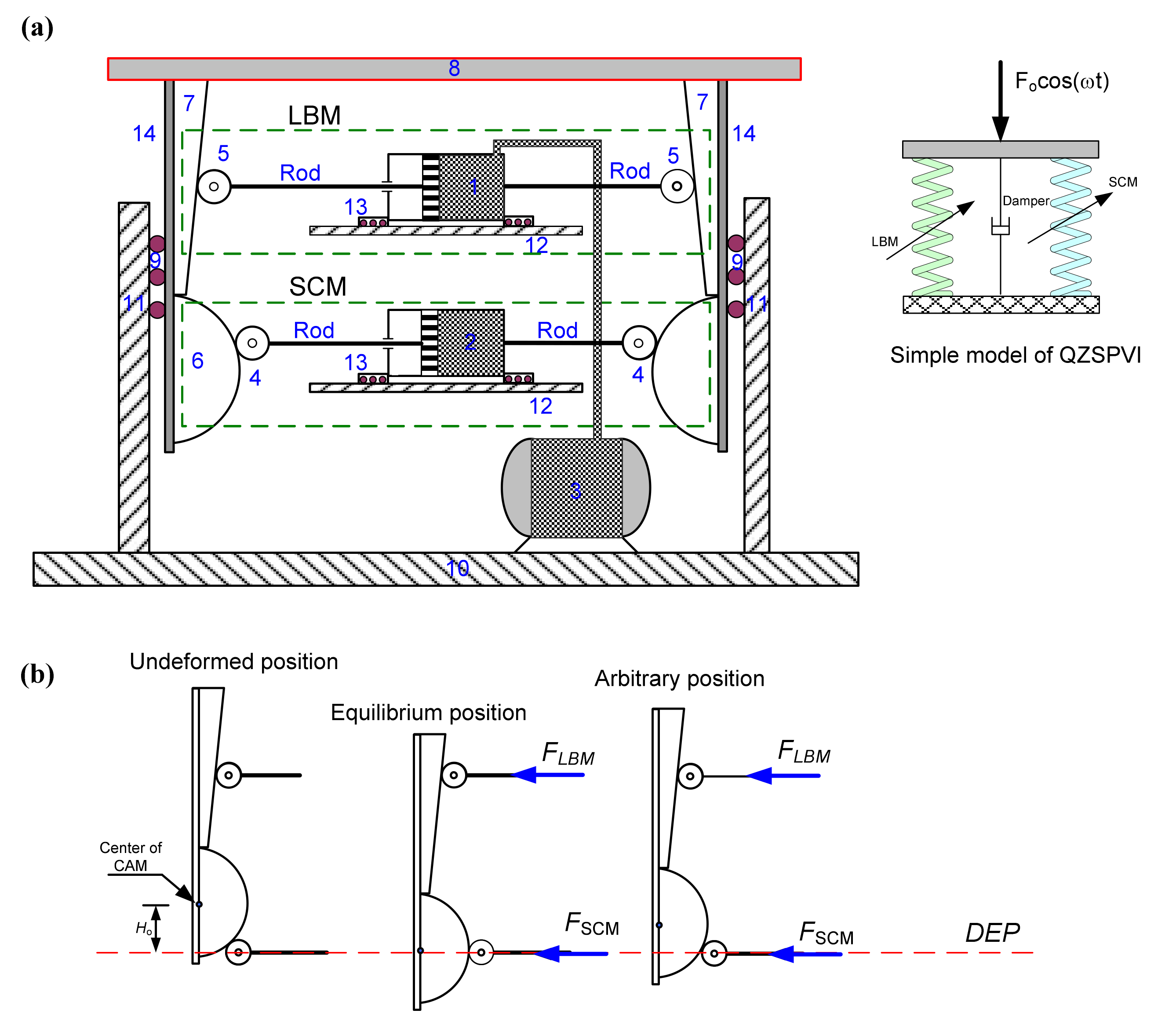
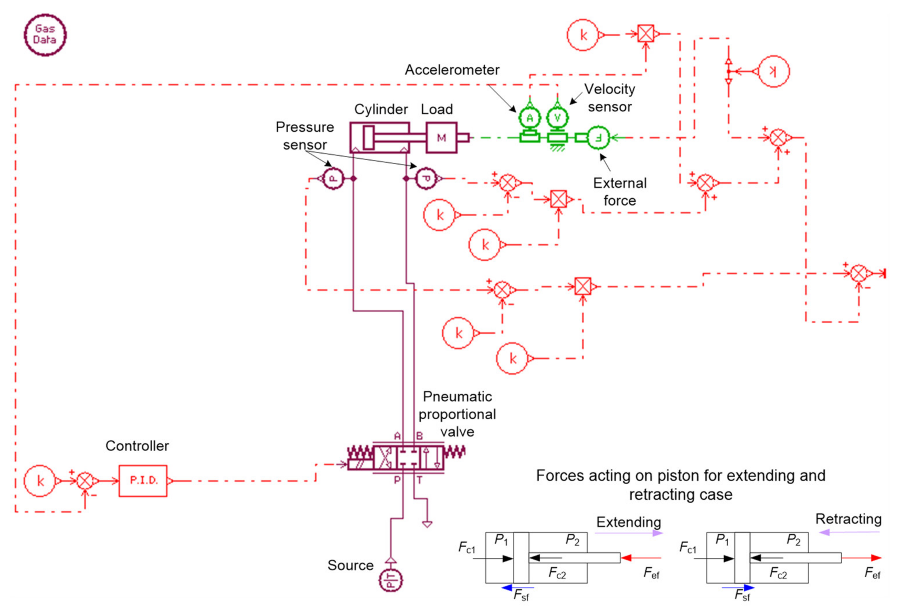
2.1. Description

The QZSPVI, which is constructed by a positive stiffness structure connecting in parallel with a negative stiffness one, is described as in Figure 1a. The formerly named load-bearing mechanism (LBM), consisting of the wedges 7, rollers 5, and cylinder 1, is used to support the load plate 8, while the latter is used to correct the dynamic stiffness of the system and is called the stiffness correction mechanism (SCM), including semicircular cams 6, rollers 4, and cylinder 2. It is noted that the wedge 7 and cam 6 are fixed on the leg 14 which is fixed on the load plate 8 and only moves vertically through the guidance bars 11 and rollers 9, meanwhile the rollers 5 and 4 only realize horizontal motion via the rods and cylinders in which the cylinders can only slide horizontally without frictional phenomenon thanks to the sliding on fixed guidance bars 12 of sliders 13. An auxiliary tank 3 connects to the cylinder 1 of the LBM to improve symmetry of the dynamic stiffness curve, and the stiffness of the QZSPVI can offer desirable low values by adjusting the low pressure in cylinders 1 and 2.
During the operation of the system, it can spend three states as shown in Figure 1b, including the undeformed, desirable equilibrium, and arbitrary position. For example, at the undeformed one, the air in the cylinders 1 and 2 is not compressed, meaning that no force is generated by the LBM and SCM. The vertical distance (Ho) between the centers of the cam 6 and roller 4 is called the static deformation of the system. The desirable equilibrium position (DEP), determined as the load plate, is loaded until the centers of cam and roller are on the same horizontal line. At this state, the vertical force which acts on the load plate is only caused by the load-bearing structure, whilst the arbitrary state is determined when the load plate moves away from the equilibrium position at distance u < Ho, at which the load plate will be acted on by two vertical forces generated by both the LBM and SCM
Supposing at an arbitrary position, the vertical forces generated by the elastic forces of the load-bearing mechanism (FLBM) and the stiffness corrected mechanism (FSCM) are determined as the following:
F s = F L B M + F S C M
As analyzed in [28], the FLBM and FSCM are expressed as below
F L B M = 2 A 1 P s o 1 A 1 h 1 + V t A 1 h 1 + V t 2 A 1 H o tan α + 2 A 1 u tan α n P a t m tan α
F S C M = 2 A 2 P s o 2 A 2 h 2 A 2 h 2 + 2 A 2 R + r 2 H o 2 2 A 2 R + r 2 u 2 n P a t m u R + r 2 u 2
in which n is the ratio of specific heat capacity, R and r are the radii of the semicircular cam and roller in m, Patm is the ambient pressure in Pa, while Pso is the pressure in cylinder at the undeformed position in Pa, the area of piston is denoted by A in m2, h is the working stroke length of piston in m as denoted in Figure 1a, Vt is the volume of the auxiliary tank, u is the relative displacement between the base and load plate. It is noted that parameters that are representative for pneumatic springs 1 and 2 are noted by subscripts “1”and “2”, respectively.
As described above, the load plated is only supported through the pressure which is generated by the LBM. Hence, it is necessary to determine the relationship between the pressure in cylinder 1 and the weight of the isolated object as expressed by Equation (4), meaning that thanks to this relation, the system can obtain the desired equilibrium position.
P e p 1 = M g 2 A 1 tan φ + P a t m
in which the pressure (Pep1) of the cylinder 1 at the equilibrium position is determined as follows:
P e p 1 = P s o 1 A 1 h 1 + V t A 1 h 1 + V t 2 A 1 H o tan α n
To ensure the load-bearing capacity in the expected working region u H o , the initial pressure Pso1 of the LBM must be larger than one. This indicates that the working parameters of the cylinder 1 must satisfy the following condition:
2 A 1 H o tan α A 1 h 1 + V t   < 1   1 P e p 1 1 / n
For instance, Ho = 73.5 mm and A1 = 0.0095 m2, through Equations (4)–(6), the relationship between the weight of the isolated load and the initial volume for which the pressure in the cylinder 1 is always higher than one as shown in Figure 2. It can be seen that either increasing the initial pressure or reducing the tank volume will result in an increase in the isolated load. However, the effect of these parameters on the isolated load is different. Specifically, the isolated load is almost increased gradually according to the growth of the initial pressure as observed in Figure 2b, created by a cutting section Vt = 0.01 m3. Meanwhile, the Figure 2c cut by a section at Pso1 = 2 bar indicated that the isolated mass can be remarkably varied, as there is a change of the tank volume in the region of less than 0.05 m3.
Similarly, the pressure in cylinder of the SCM must be always larger than one for the remaining function of correcting the dynamic stiffness of the SCM. The working region of the SCM is predicted as following:
u u L _ S C M = R + r 2 A 2 h 2 + 2 A 2 ( R + r ) 2 H o 2 V e p 2 P e p 2 P a t m 1 / n 2 A 2 2
herein Pep2 and Vep2 are denoted as the pressure and volume in the cylinder 2 at the equilibrium position.

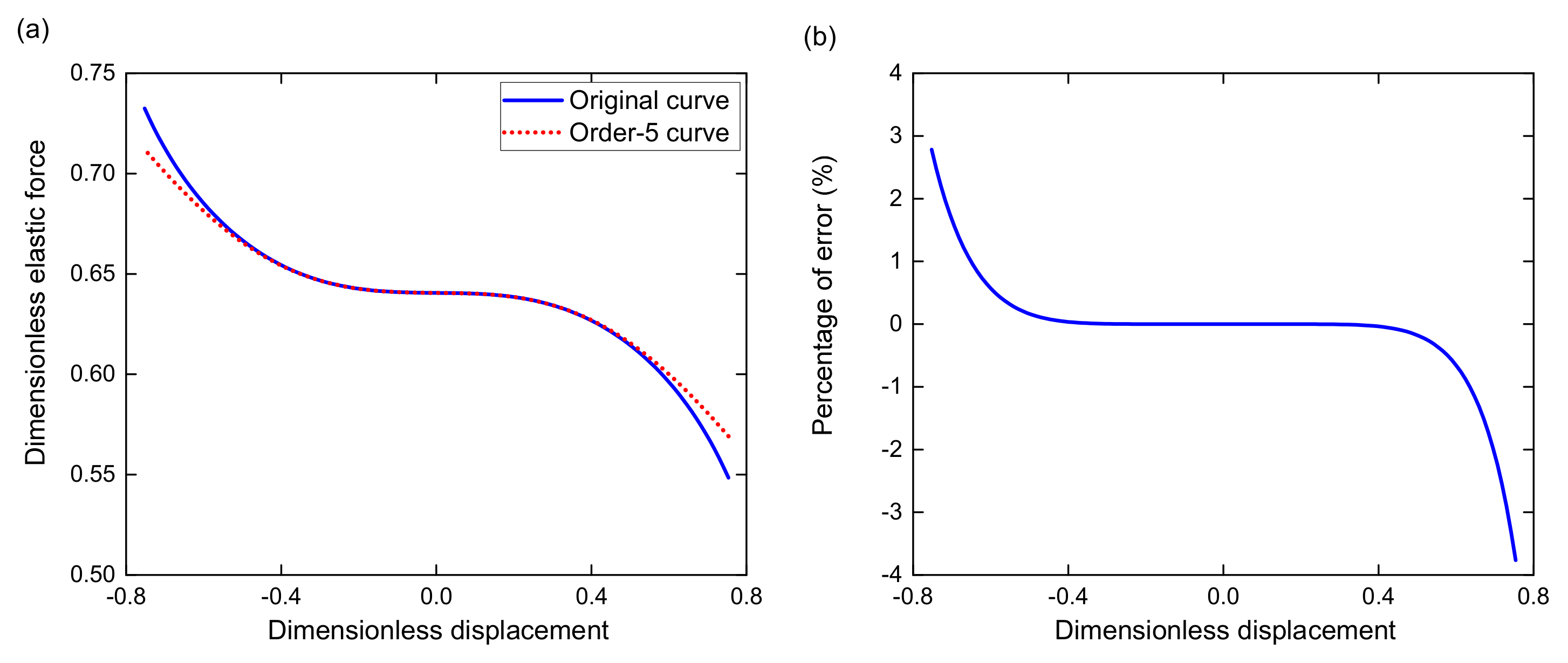
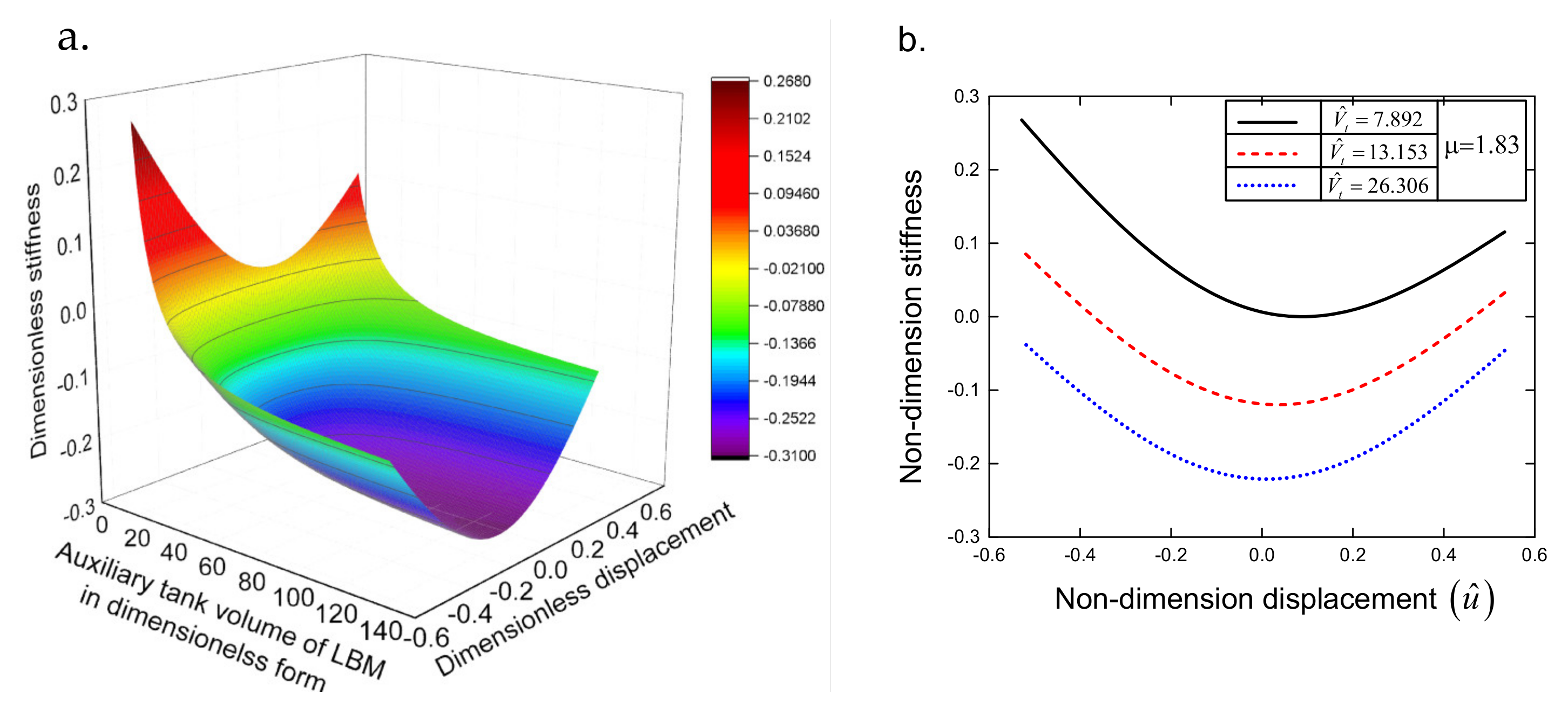
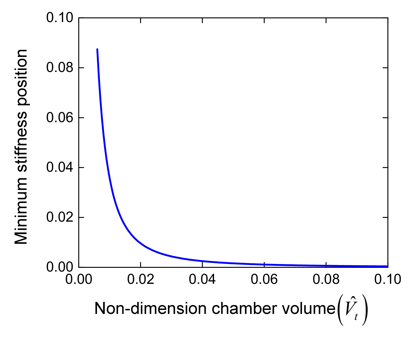
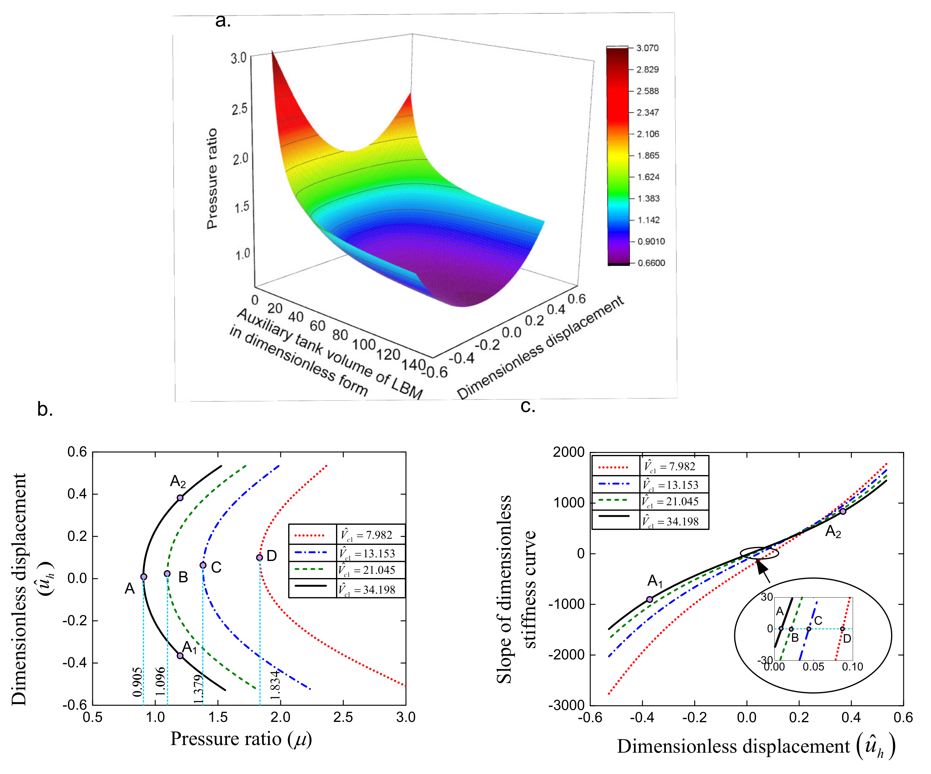
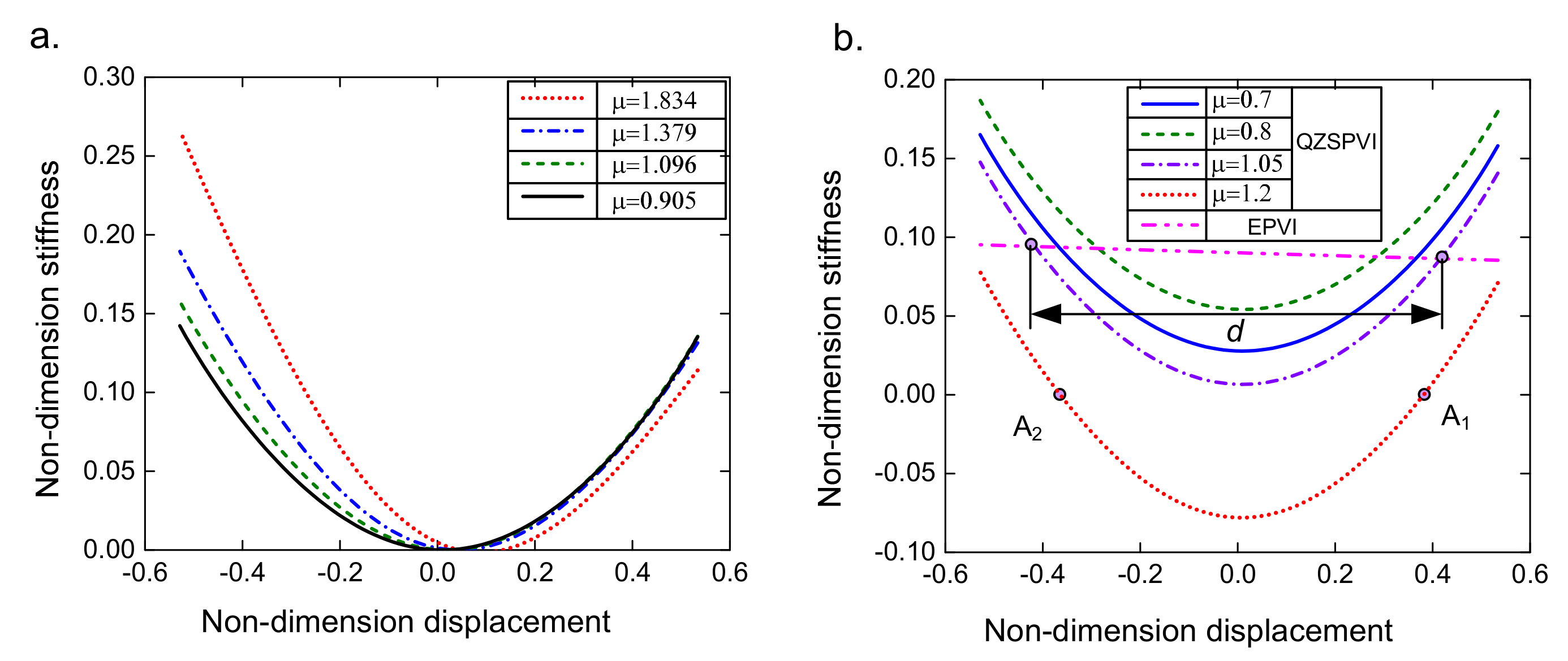
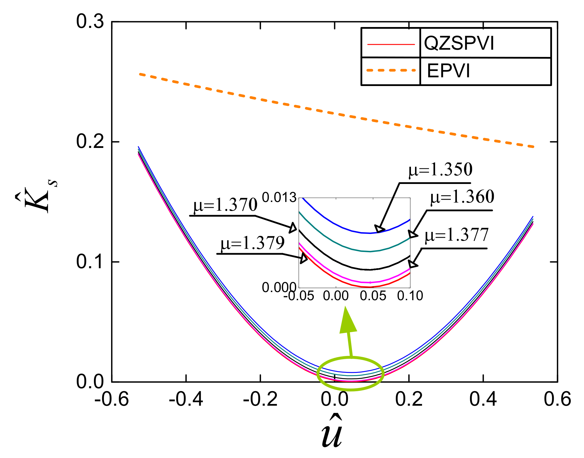
2.2. Stiffness Analysis

Taking a derivation of Equation (1) versus dimensionless displacement u ^ , the vertical stiffness is expressed in the form of dimensionless as following:
K ^ s = 4 n V ^ n e p 1 V ^ c y 1 + V ^ t n tan 2 α V ^ c y 1 + V ^ t 2 H ^ o tan α + 2 u ^ tan α n + 1 + 2 A ^ 1 u ^ 2 P ^ a t m μ V ^ e p 2 n V ^ c y 2 V ^ c y 2 + 2 A ^ 1 H ^ o 2 2 A ^ 1 u ^ 2 n 1 1 u ^ 2 + u ^ 2 1 u ^ 2 4 n μ A ^ 2 V ^ e p 2 n V ^ n c y 2 V ^ c y 2 + 2 A ^ 1 H ^ o 2 2 A ^ 1 u ^ 2 n + 1
in which
K ^ S = K S b A 1 P d 1 A ^ = A 2 A 1 ;   H ^ o = H o R + r ;   P ^ a t m = P a t m P d 1 ;   u ^ = u R + r ;   V ^ c y 1 = V c y 1 A 1 ( R + r ) ;   V c y 1 = A 1 h 1 ;   V ^ c y 2 = V c y 2 A 1 ( R + r ) ;   V c y 2 = A 2 h 2 ; V ^ t = V t A 1 ( R + r ) ;   V ^ e p 1 = V e p 1 V c y 1 + V t ;   V ^ e p 2 = V e p 2 V c y 2 ; F ^ L B M = F L B M A 1 P e p 1 ;   μ = P e p 2 P e p 1 .
In order to simplify the dynamic analysis in the next section, the restoring force given by Equation (1) can be expressed approximately (Fap) by expanding the Taylor series around the wanted equilibrium position u = 0 as below:
F a p = F o + a 1 u + a 2 u 2 + a 3 u 3 + a 4 u 4 + a 5 u 5 + O ( u 6 )
herein,
F o = 2 A 1 P s o 1 A 1 h 1 + V t A 1 h 1 + V t 2 A 1 H o tan α n P a t m tan α a n = 1 n d F L B M n d u n + d F S C M n d u n u = 0 n = 1 , 2 , 3 , 4 , 5
The original elastic force given by Equation (1) and its approximated form expressed by Equation (9) are compared as in Figure 3a. The former is denoted by the solid line, while the latter is drawn by the dot line. It is interesting to see that the curve of Equation (1) is approximated to 5th order through expanding Taylor series, which is in good agreement with the other. Furthermore, the error percentage of the approximated curve is lower than 4% compared with the exact solution, as shown in Figure 3b. As observed, at the equilibrium position, the error is equal to zero, but when moving away from this position, error is increased. Indeed, within u ^ = 0.5 ÷ 0.5 , the slope of the force curve is very low. Meanwhile, out of this region, the slope is increased significantly as shown in Figure 3a, indicating that the rate of changing error within u ^ = 0.5 ÷ 0.5 is also very low, outside it is developed strongly. This means that the 5th order polynomial is suitable for small amplitude oscillation. This approximated solution will be used for analyzing the primary resonance response of the proposed system.
Figure 4a shows the dynamic stiffness surface in the space V ^ t , u ^ , K ^ s in which the pressure ratio µ is 1.83, and other parameters include V ^ c y 1 = 1.875 ;   V ^ c y 2 = 0.248 . It revealed that the stiffness of the QZSPVI is strongly affected by the auxiliary tank volume Vt of the load-bearing mechanism. Reducing the value of Vt will increase the value of the system stiffness. Simultaneously, the asymmetric level of the stiffness curve around the equilibrium position is also developed. This is seen clearly in Figure 4b, and created by cutting sections at V ^ t = 7.892 ,   13 . 153 ,   26 . 306 (types of lines are presented in the top-right corner panel). Furthermore, because of the asymmetry of the stiffness curve, the system can not achieve the lowest stiffness at the equilibrium position (u = 0). As observed, for the 1st dimensionless value of the tank volume, the position defined by u ^ l s at which the stiffness achieving the lowest value is approximated 0.084 and the value of u ^ l s can be reduced to 0.034 and 0.09 as the auxiliary tank volume is grown to 13.153 and 26.306, respectively.
The lowest stiffness position can be predicted by differentiating Equation (9) to second order versus the displacement as expressed in Equation (11), and then it equals zero. It can be seen that this position will be asymptotic to the wanted equilibrium position when the auxiliary tank volume V ^ t is large enough, as shown in Figure 5.
2 a 2 + 6 a 3 u + 12 a 4 u 2 + 20 a 5 u 3 = 0
In addition, from Equation (8) for Pe1 = 2 bar, by setting Ks = 0, the relationship between the pressure ratio and the auxiliary tank volume for which the pressure in cylinder of the SCM will be calculated is marked in Figure 6a. The pressure ratio curve is formed by cutting sections at the various values of the auxiliary tank volume V ^ t as shown in Figure 6b, in which the values of V ^ t and the notation for line types are noted in the middle of the panel. It can be observed that in the case of V ^ t = 34.198 , at the extremum point A corresponding to the pressure ratio µ = 0.905, the oscillation system can obtain the quasi-zero stiffness at only one position u ^ A = 0.008 but µ > 0.905, there may exist two positions at which the stiffness is also nearly equal to zero such as at point A1  u ^ = 0.381 and point A2 ( u ^ = 0.364 ) for µ = 1.2. It is shown that lessening the volume V ^ t leads to the increase of the pressure ratio. For instance, V ^ t = 21.045 ,   13 . 153 , and 7.982, the lowest pressure ratios to obtain quasi-zero stiffness are 1.096, 1.379, and 1.834 are marked by the extremum point such as B, C, and D, respectively. The slope of the stiffness curve at points A u ^ A = 0.008 , B u ^ B = 0.021 , C u ^ C = 0.046 , D u ^ D = 0.083 is nearly equal to zero as depicted in Figure 6c (all parameters are the same as in Figure 6b). Meanwhile, for other positions (A1, A2, etc.) these are nonzero, indicating that for the value of µ at extreme points of the pressure ratio curve, the dynamic stiffness is equal to zero and obtains the minimum value in the expected working region. This result is also confirmed in Figure 7a, herein the values of µ and annotation of the line types are given in the top right corner panel of the figure.
As mentioned above, points may exist where the stiffness of the QZSPVI is quasi-zero but the slope of the stiffness curve is nonzero. For example, for µ = 1.2, V ^ t = 34.198 , the system has quasi-zero stiffness at the position A1 ( u ^ = 0.381 ) and A2 ( u ^ = 0.364 ) (seen in Figure 6b), but at which the slope of the stiffness curve is larger than zero at A2 and smaller than zero at A1 (seen in Figure 6c). The result is an area from the position A1 to A2 in which the dynamic stiffness of the QZSPVI is negative, as shown by a dot line in Figure 7b. On the aspect of isolation, this case is not suitable for designing an isolated model due to its unstableness. Besides, if the pressure ratio is chosen so that its value is smaller than that at the extremum point of the pressure ratio curves, the stiffness of the system is always larger than zero as exhibited in the Figure 7b herein, the value of µ is chosen 0.7 (solid line), 0.8 (dashed line), and 1.05 (dash-dot line), while the dimensionless value of the auxiliary tank volume is 34.198. Furthermore, it is interesting to note that the region d in which the dynamic stiffness of the QZSPVI is smaller than that of the EPVI (plotted by dash-dot-dot line) is increased according to the increase in the pressure ratio.

3. Dynamic Analysis

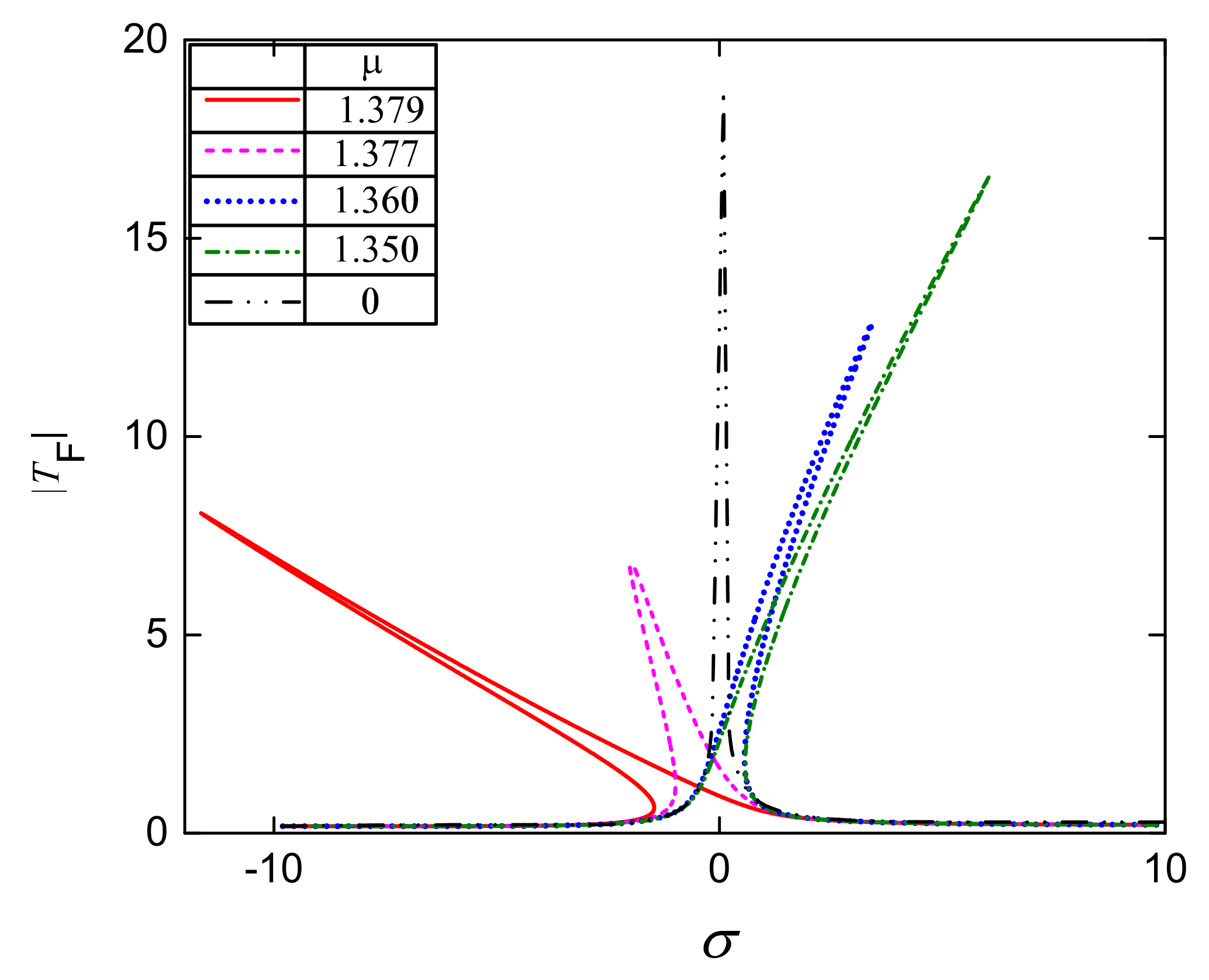
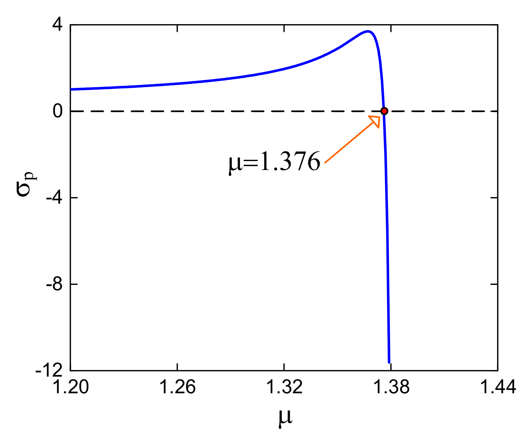
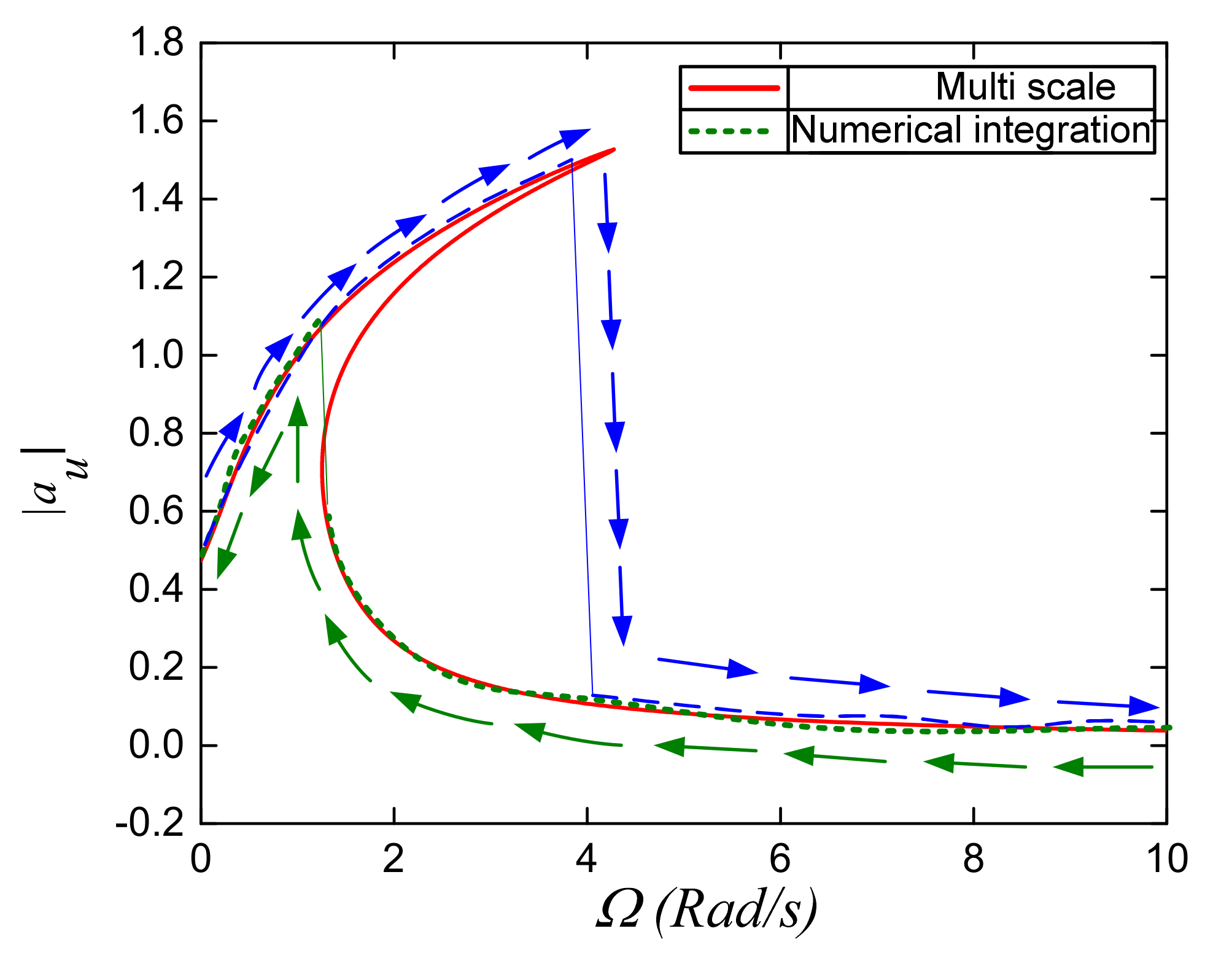
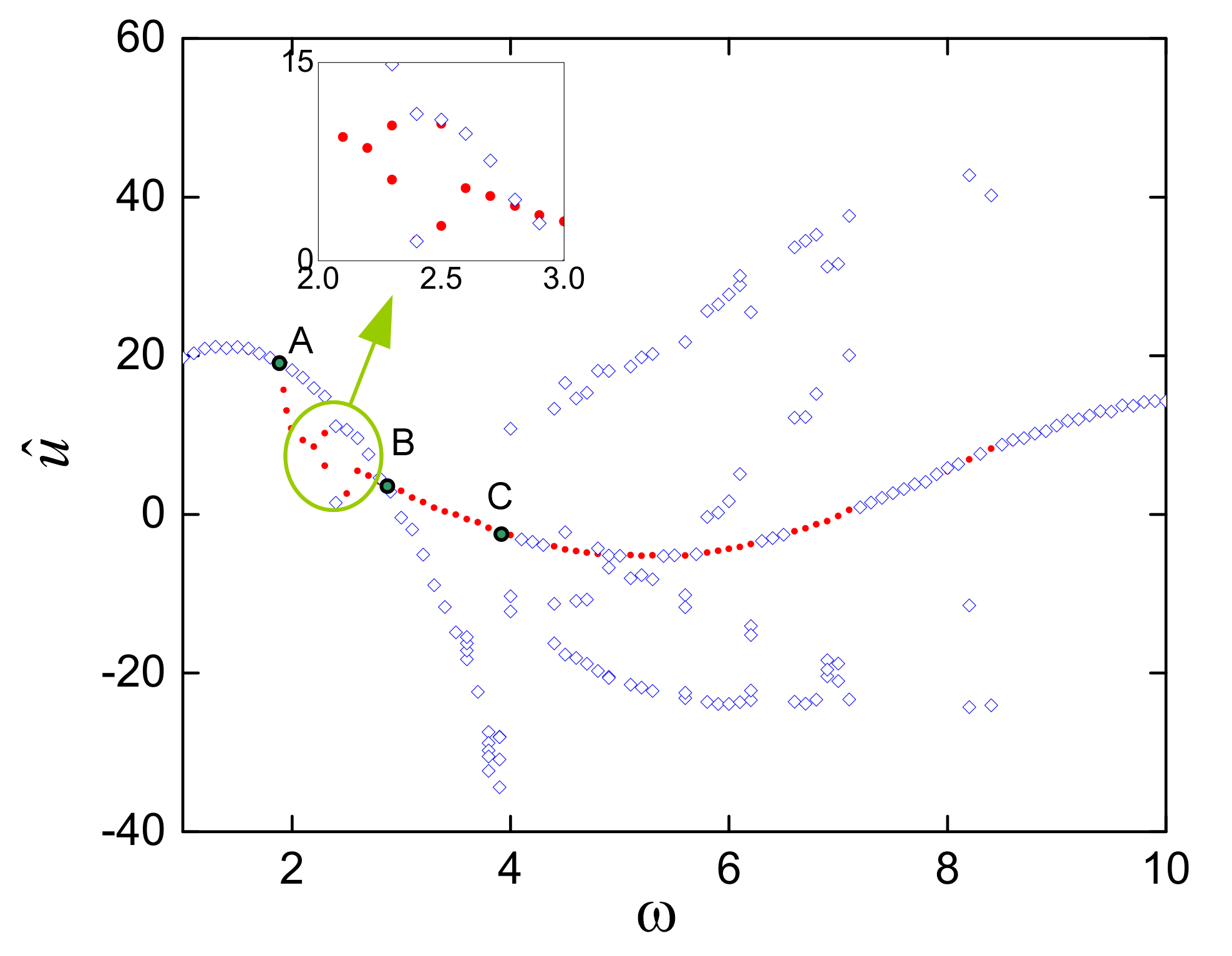
3.1. Primary Frequency—Amplitude Relation

Considering that the load plate is acted by a harmonic force with the amplitude Fe and frequency ω, the motion of the load plate is expressed as following:
M u ¨ + C u ˙ a 1 u + a 2 u 2 + a 3 u 3 + a 4 u 4 + a 5 u 5 = F e cos ω t
By introducing parameters as following:
u ^ = u u o ;   ω n 2 = a 1 M ;   Ω = ω ω n ;   τ = ω n t ;   ξ = C 2 ω n M ; α n = a n u o n 1 M ω n 2 ;   u o = F e a 1 ω = 0 ; a i = 0 ( i = 2 , 3 , , 5 )
In dimensionless form, Equation (12) is rewritten as below:
u ^ + 2 ξ u ^ + u ^ + n = 2 5 α n u ^ n = c o s Ω τ
where the number of primes denote the order of differentiation with respect to dimensionless time τ
In order to find the solution in the neighborhood of the equilibrium position u ^ = 0 , we let u ^ = ε x ^
x ¯ + 2 ε 4 ξ ˜ x ¯ + x ¯ + n = 2 5 α n ε n 1 x ¯ n = ε 4 k ˜ cos Ω τ
herein ε << 1, and ε 4 ξ ˜ x ¯ = ξ x ^ ;   cos ( Ω τ ) = ε 4 k cos ( Ω τ ) .
By applying the multi-scale method, the approximated solution of Equation (14) is obtained as following:
x ^ ( τ , ε ) = x ^ o ( T o , T 1 , T 2 , T 3 , T 4 ) + ε x ^ 1 ( T o , T 1 , T 2 , T 3 , T 4 ) + ε 2 x ^ 2 ( T o , T 1 , T 2 , T 3 , T 4 ) + ε 3 x ^ 3 ( T o , T 1 , T 2 , T 3 , T 4 ) + ε 4 x ^ 4 ( T o , T 1 , T 2 , T 3 , T 4 ) + + O ( ε 5 )
in which T i = ε i τ   ( i = 0 , 1 , 2 , 3 , 4 ) . Substituting Equation (15) into Equation (14) and letting Ω = 1 + ε2σ then equating the coefficient of εo, ε1, ε2, ε3, ε4 on both sides of the equation, yields
ε o D o 2 x ^ o + x ^ o = 0 ε 1 D o 2 x ^ 1 + x ^ 1 = 2 D o D 1 x ^ o α 1 x ^ o ε 2 D o 2 x ^ 2 + x ^ 2 = 2 D o D 1 x ^ 1 2 D o D 2 x ^ o D 1 2 x ^ o α 1 x ^ o x ^ 1 α 2 x ^ o 3 ε 3 D o 2 x ^ 3 + x ^ 3 = 2 D o D 1 x ^ 2 2 D o D 2 x ^ 1 2 D o D 3 x ^ o 2 D 1 D 2 x ^ o D 1 2 x ^ 1 α 1 x ^ 1 2 + 2 x ^ o x ^ 2 3 α 2 x ^ o 2 x ^ 1 α 3 x ^ o 4 ε 4 D o 2 x ^ 4 + x ^ 4 = 2 D o D 1 x ^ 3 2 D o D 2 x ^ 2 2 D o D 3 x ^ 1 2 D o D 4 x ^ o 2 D 1 D 2 x ^ 1 2 D 1 D 3 x ^ o 2 ξ ˜ D o x ^ o - D 1 2 x ^ 2 D 2 2 x ^ o α 1 2 x ^ o x ^ 3 + 2 x ^ 1 x ^ 2 3 α 2 x ^ o 2 x ^ 2 + x ^ o x ^ 1 2 4 α 3 x ^ o 3 x ^ 1 α 4 x ^ o 5 + K ˜ cos ( T o + σ T 2 )
where D i n = n d T i n i = 1, 2, 3, 4; n is the order of the differentiation
The general solution of the first equation in Equation (16) is expressed as below:
x ^ o = A ^ T 1 , T 2 , T 3 , T 4 , e i T o + A ^ ¯ T 1 , T 2 , T 3 , T 4 , e i T o
where A ^ is an unknown complex amplitude and A ^ ¯ is the complex conjugate of A.
Substituting Equation (17) into the second equation in Equation (16), we obtain the following:
D o 2 x ^ 1 + x ^ 1 = 2 D 1 A ^ e i T o i α 1 A ^ 2 e 2 i T o + 2 A ^ A ^ ¯ + A ¯ 2 e 2 i T o + 2 D 1 A ^ ¯ e i T o i
In order to obtain the periodic solution of Equation (18), imaginary terms in the right side of Equation (18) must be zero. Namely,
D 1 A ^ = 0 ;   D 1 A ^ ¯ = 0 A ^ ( T 2 , T 3 , T 4 )
In the same way of the solution for ε1-order equation, from ε2, ε3, and ε4 order equations, we have:
2 D 2 A ^ i = 10 α 1 2 A ^ 2 A ^ ¯ 3 3 α 2 A ^ 2 A ^ ¯ ;   2 D 2 A ^ ¯ i = 10 α 1 2 A ^ A ^ ¯ 2 3 + 3 α 2 A ^ A ^ ¯ 2 2 D 3 A ^ i = 0 2 D 4 A ^ i = 2 ξ ˜ A i + 10 α 1 2 6 3 α 2 2 2 A ^ 3 A ^ ¯ 2 α 1 26 α 1 α 2 12 1172 α 1 3 216 28 α 3 3 A ^ 3 A ^ ¯ 2 - α 2 1926 α 1 2 216 + 3 α 2 8 A ^ 3 A ^ ¯ 2 56 α 1 α 3 3 A ^ 3 A ^ ¯ 2 10 α 4 A ^ 3 A ^ ¯ 2 + K ˜ 2 e i σ T 2
The case in which the complex amplitude can be expressed as A ^ = 1 2 a ^ e i β ,   A ^ ¯ = 1 2 a ^ e i β with a and β are real, then separating the real and imaginary parts, the differential equation for amplitude and frequency of Equations (19) and (20) are expressed as below:
D 1 a ^ = 0 ;   a ^ D 1 β = 0 D 2 a ^ = 0 ;   a ^ D 2 β = 3 α 2 a ^ 3 8 10 α 1 2 a ^ 3 24 D 3 a ^ = 0 ; a ^ D 3 β = 0 D 4 a ^ = ξ ˜ a ^ + 1 2 K ˜ sin σ T 2 β a ^ D 4 β = 10 α 1 2 6 3 α 2 2 2 1 2 5 a ^ 5 + α 1 26 α 1 α 2 12 1172 α 1 3 216 28 α 3 3 1 2 5 a ^ 5 + α 2 1926 α 1 2 216 + 3 α 2 8 1 2 5 a ^ 5 + 56 α 1 α 3 3 1 2 5 a ^ 5 + 10 α 4 2 5 a ^ 5 1 2 K ˜ cos σ T 2 β
In addition, the differentiation of a and β with respect to dimensionless time τ is presented as below:
a ^ = d a d τ = ε D 1 a ^ + ε 2 D 2 a ^ + ε 3 D 3 a ^ + ε 4 D 4 a ^ β = d β d τ = ε D 1 β + ε 2 D 2 β + ε 3 D 3 β + ε 4 D 4 β
From Equation (21), Equation (22) is rewritten as the following:
a ^ = ξ ˜ ε 4 a ^ + 1 2 ε 4 K ˜ sin σ T 2 β a ^ β = 3 α 2 8 ε 2 a ^ 3 10 α 1 2 24 ε 2 a ^ 3 + 10 α 1 2 6 3 α 2 2 2 1 2 5 ε 4 a ^ 5 + ε 4 α 1 26 α 1 α 2 12 1172 α 1 3 216 28 α 3 3 1 2 5 ε 4 a ^ 5 + α 2 1926 α 1 2 216 + 3 α 2 8 1 2 5 ε 4 a ^ 5 + 56 α 1 α 3 3 1 2 5 ε 4 a ^ 5 + 10 α 4 2 5 ε 4 a ^ 5 ε 4 K ˜ 2 cos σ T 2 β
Recalling u ^ = ε x ^ , and by letting γ = σ T 2 β , Equation (23) is expressed with respect to a ^ u as below:
a ^ u = ξ a ^ u + 1 2 K sin γ a ^ u γ = a ^ u σ G ( α 1 , α 2 ) a ^ u 3 F ( α 1 , α 2 ) a ^ u 5 + K 2 cos γ
with a ^ u = ε a , G ( α 1 , α 2 ) = 3 α 2 8 10 α 1 2 24 ;
F ( α 1 , α 2 ) = 10 α 1 2 6 3 α 2 2 2 1 2 5 + ε 4 α 1 26 α 1 α 2 12 1172 α 1 3 216 28 α 3 3 1 2 5 + α 2 1926 α 1 2 216 + 3 α 2 8 1 2 5 + 56 α 1 α 3 3 1 2 5 + 10 α 4 2 5
The solution of Equation (13) is:
u ^ = a ^ u cos ( Ω τ γ )
As the amplitude and phase are unchanged, the steady state motion will occur, meaning that
1 2 K sin γ = ξ a ^ u K 2 cos γ = G ( α 1 , α 2 ) a ^ u 3 + F ( α 1 , α 2 ) a ^ u 5 a ^ u σ
The frequency–response relationship of Equation (14) is obtained as follows:
ξ a ^ u 2 + G ( α 1 , α 2 ) a ^ u 3 + F ( α 1 , α 2 ) a ^ u 5 a ^ u σ 2 = 1 4 K 2
From Equation (28), we have:
σ 1 , 2 = G ( α 1 , α 2 ) a ^ u 3 + F ( α 1 , α 2 ) a ^ u 5 ± 1 4 K 2 ξ a ^ u 2 a u
The peak amplitude ( a ^ u p ) and frequency (σp) are calculated as below:
a ^ u p = 1 2 ξ K σ p = G ( α 1 , α 2 ) a ^ u p 3 + F ( α 1 , α 2 ) a ^ u p 5 a u p
Considering a ^ u o & γ o along with a set of steady state solutions and its neighborhood are determined by introducing small variations a ^ u 1 & γ u 1 as follows:
a ^ u = a ^ u o + a ^ u 1 γ = γ u o + γ u 1
To accomplish the stable analysis, Equation (24) is rewritten as
a ^ u o = ξ a ^ u o + a ^ u 1 + 1 2 K sin γ u o + γ u 1 γ = σ G ( α 1 , α 2 ) a ^ u o + a ^ u 1 2 F ( α 1 , α 2 ) a ^ u o + a ^ u 1 4 + K 2 a ^ u o + a ^ u 1 cos γ u o + γ u 1
Based on Routh–Hurwitz criterion for nonlinear system, the stability of the steady state solution depending on the eigenvalues λ is determined as below:
ξ λ G ( α 1 , α 2 ) a ^ u 3 + F ( α 1 , α 2 ) a ^ u 5 a ^ u σ 2 G ( α 1 , α 2 ) a ^ u o 4 F ( α 1 , α 2 ) a ^ u o 3 K 2 a ^ u o 2 cos γ u o ξ λ = 0
The unstable region of the steady state motion above is obtained as follows:
ξ 2 + 2 G ( α 1 , α 2 ) a ^ u o + 4 F ( α 1 , α 2 ) a ^ u o 3 + K 2 a ^ u o 2 cos γ u o G ( α 1 , α 2 ) a ^ u 3 + F ( α 1 , α 2 ) a ^ u 5 a ^ u σ < 0

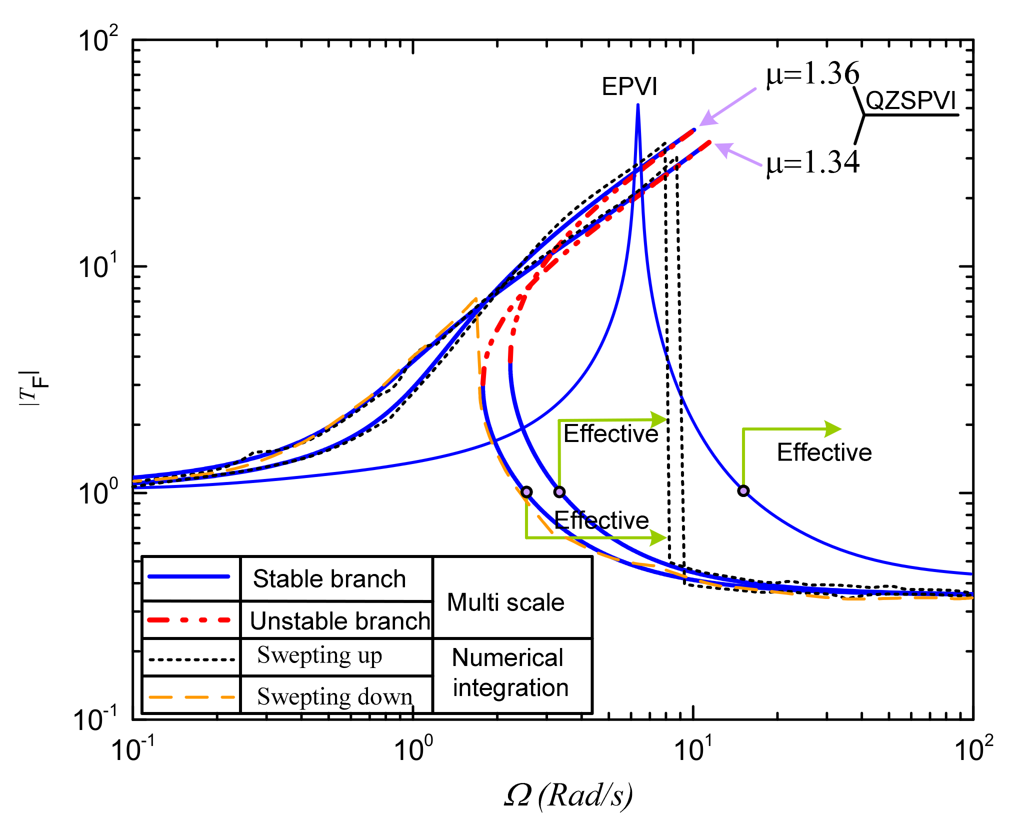
3.2. Transmissibility for Force Excitation

The case of the QZSPVI is subjected to a harmonic forcing excitation F = Fe cos(ω). Through the LBM, SCM, and air damping, the force is transmitted to the base and can be written in dimensionless form as below:
F t = 2 ξ u ^ + u ^ + n = 2 5 α n u ^ n
It reveals that the transmitted force depends on the velocity and position of the load plate given in Equation (26). This force may be rewritten as:
F ^ t = 2 ξ a u Ω sin ( Ω τ γ ) + a ^ u + 3 α 3 a ^ u 3 4 + 7 α 5 a ^ u 5 8 cos ( Ω τ γ )
The maximum force is transmitted to the base, being:
F ^ t max = 2 ξ a ^ u Ω 2 + a ^ u + 3 α 3 a ^ u 3 4 + 7 α 5 a ^ u 5 8 2
The transmissibility for forcing excitation is defined as below:
| T F | = F ^ t max F ^ e
herein from Equation (4), the non-dimensional magnitude of the excited force F ^ e = 1

4. Numerical Simulation

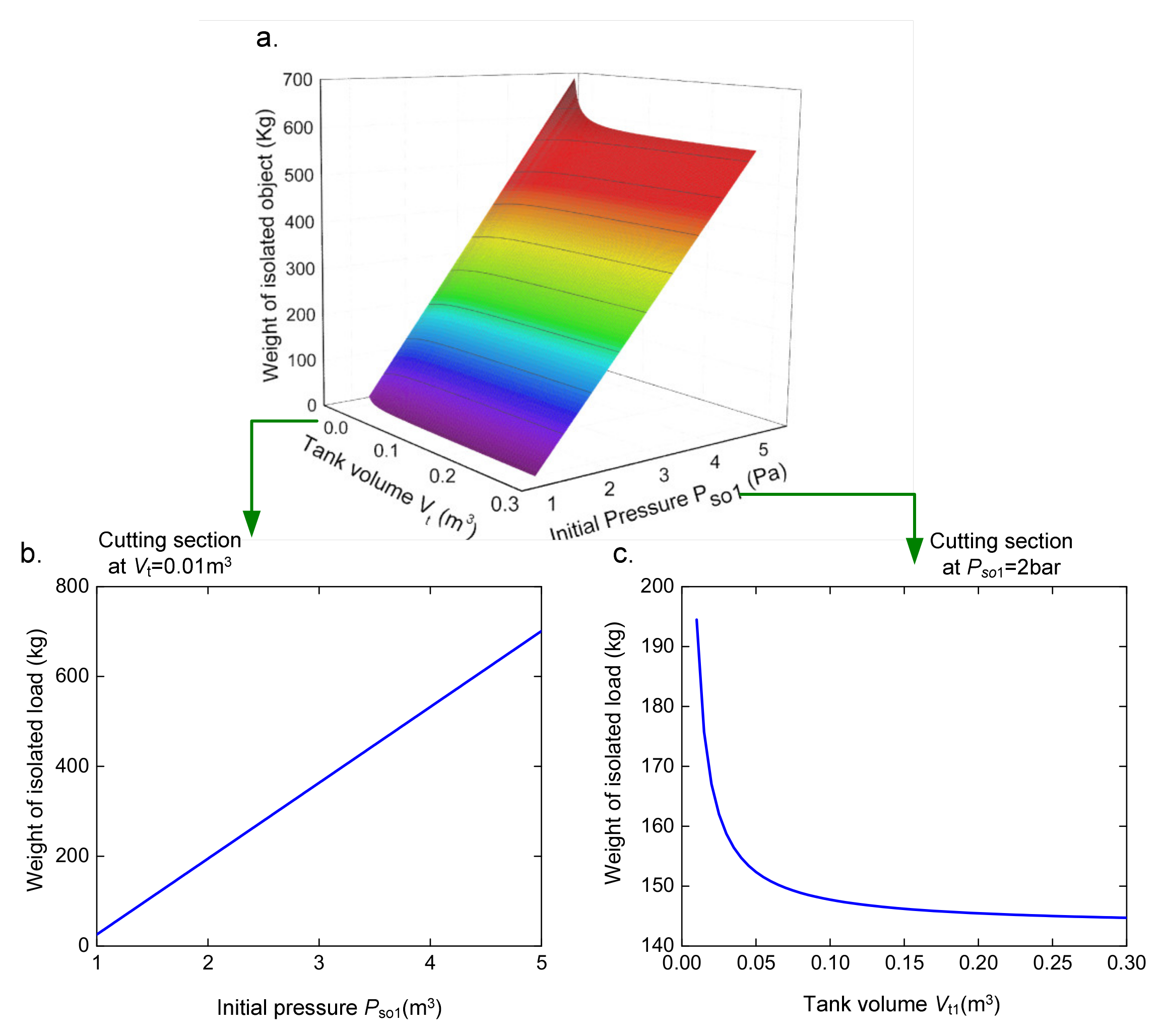
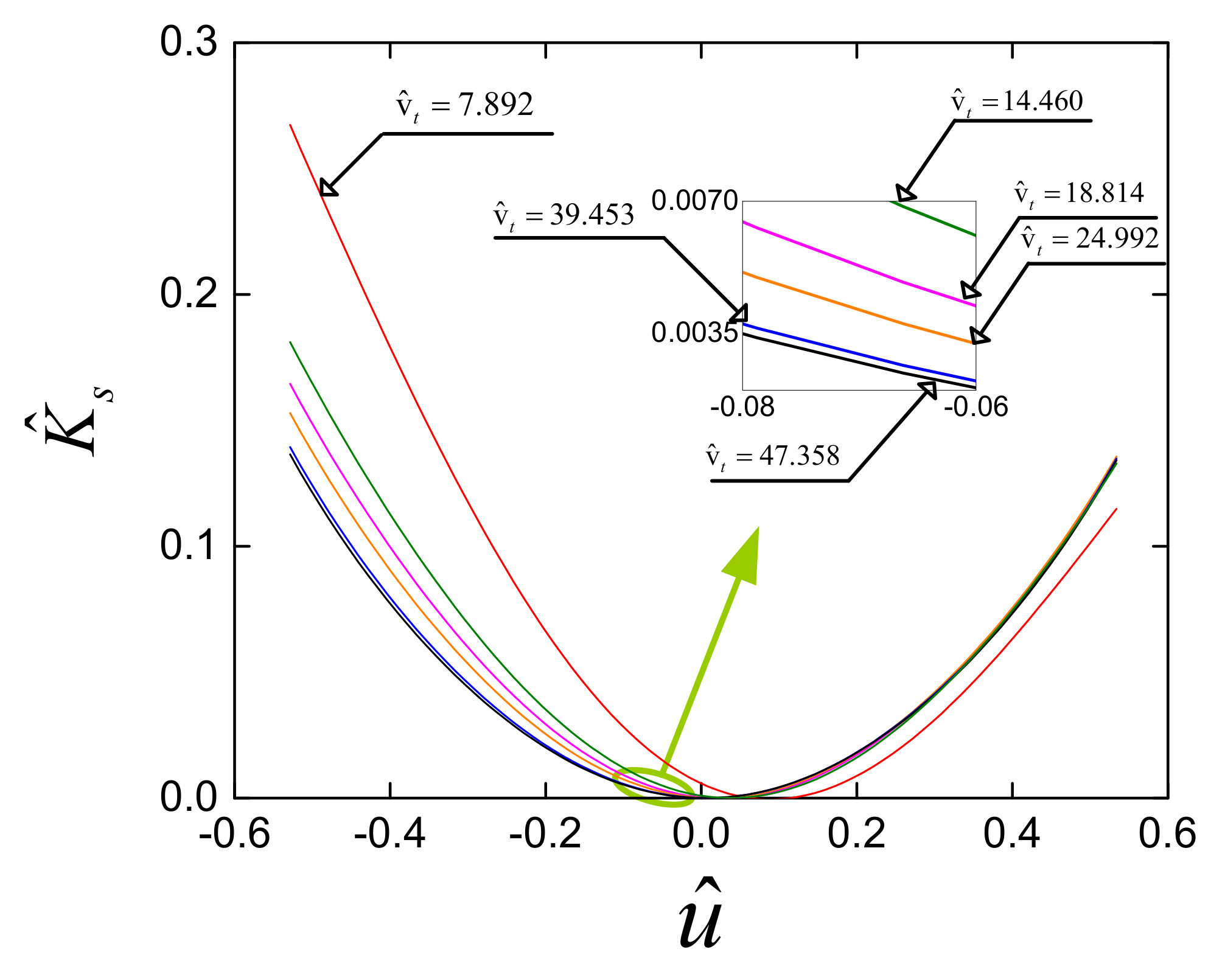
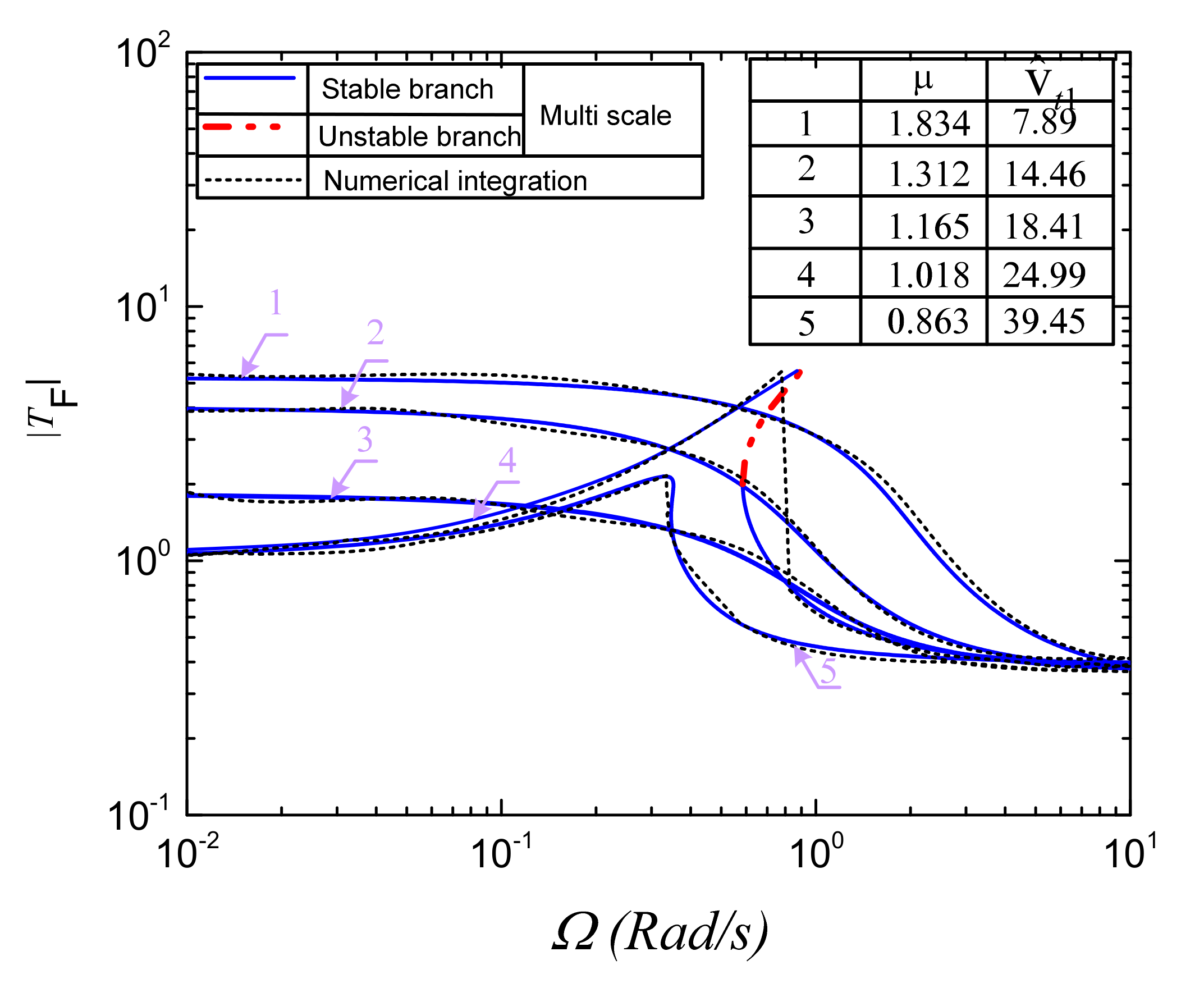
4.1. Influence of Parameters on the Force Transmitted Curve

In this section, the effects of the pressure ratio and volume of auxiliary tank on the force transmissibility of the QZSPVI are investigated. Firstly, the pressure ratio will be studied. Meanwhile, a set of parameters of the isolation system comprising of ξ = 0.1 ;   A ^ = 0.16 ;   V ^ t = 13.153 ;   H ^ o = 0.53 is given, simultaneously at the equilibrium position, the pressure Pep1 of the LBM is set at the value of 1.85 bar, for which the weight of the isolated load is 122.41 kg. As observed in Figure 8, the dynamic stiffness (denoted by the solid line) of the QZSPVI for various values of µ within 1.350 to 1.377 is always smaller than that of the EPVI (exhibited by the dashed line) when the position of the load plate is in the working region ( u ^ < H ^ o ). Especially, when µ = 1.379, the minimum stiffness of the QZSPVI is nearly equal to zero and it will be increased according to reduction in the pressure ratio. The result is the force transmitted curves shown in Figure 9 (the detailed annotation of the type of lines and the chosen values of µ are presented in the left-upper corner panel of the figure). It can be argued that the nonlinearity of the proposed model bends the force transmitted curves to the left or the right depending on the pressure ratio. In the case of µ = 1.379, the curve is bent to the left, indicating that this is the case of the soft nonlinear system. Reducing the pressure ratio will lead to reducing the soft nonlinearity to become the hard nonlinearity. As observed, the amplitude–frequency curve is bent to the right for µ = 1.370. However, the bending level of the response curve to the right may be lessened as there is a lessening in the pressure ratio such as µ = 1.360, µ = 1.350, and even trends no bending for µ = 0, as shown in Figure 9. This is evident because the pressure of the stiffness corrected mechanism will be reduced according to the reduction in the value of µ, meaning that the effects of this mechanism on the dynamic stiffness of the QZSPVI become light, and hence, the peak amplitude is increased. Furthermore, the increase of the pressure ratio will broaden the isolation region of the hardening system toward the low frequency as plotted in Figure 10. On the other hand, the comparison between the proposed system with the EPVI in which the SCM is removed is shown in Figure 10. It is noteworthy to observe that the suppression of the force transmissibility from the load plate to the base of the QZSPVI is better than the EPVI, meaning that isolation region and vibration attenuated ratio of the former is larger than those of the latter.
As analyzed above, the amplitude–frequency response of the proposed system can be soft or hard depending on the peak frequency σp. Indeed, this value is negative corresponding to the response curve bending to the left. Contrastingly, the bending to the right appeared for the positive value of σp. Figure 11 shows the influence of the pressure ratio on the peak frequency of the QZSPVI for the same parameters as in Figure 8. It is interesting to see that if the pressure ratio is larger than 1.376, the value of σp is negative, indicating that the response curve is bent to the left as confirmed in Figure 9. Meanwhile, the bending of the curve to the right occurred for µ < 1.376 due to σp > 0.
Secondly, the dimensionless volume of the auxiliary tank of the load-bearing mechanism is set at the values 7.892; 14.460; 18.814; 24.992; 39.453; 47.358, while the other values for the pressure ratio are the same as in the first case. In this case, the pressure ratio is calculated through Equation (8) as shown in Figure 12 for which in the working region, the minimum stiffness of the QZSPVI will be nearly equal to zero, as depicted in Figure 13. It is noteworthy to see that the asymmetry of the system around the equilibrium position is reduced according to the increase in the volume of the auxiliary tank, indicating that the position at which the dynamic stiffness is quasi-zero moves towards the equilibrium position.
In this case, the peak frequency and amplitude curve, with respect to the tank volume of the QZSPVI having the dynamic stiffness curves shown in Figure 13, is presented in Figure 14. It can be seen that if the dimensionless volume of the auxiliary tank is larger than 21.24 and smaller than 43.85 the value of σp is positive, but this value is negative because the volume of auxiliary tank is out of this range, as shown in Figure 14a. Besides, increasing the tank volume will lead to a lessening in the peak amplitude as observed in Figure 14b, while this may have no appearance in the peak frequency. For instance, with V ^ t = 13.5 the value of σp is around −10.5, but if V ^ t = 13.6 , this value is nearly equal to −21. Furthermore, as the dimensionless volume of the auxiliary tank is changed from 43.83 (at point A) to 43.88 (at point B), the value of σp is changed suddenly from positive to negative. Simultaneously, the peak amplitude is decreased remarkably. In addition, it is essential to note that increasing the auxiliary tank volume will extend the region isolation toward low frequency, as shown in Figure 15. This indicates that improving the symmetry of the stiffness curve will increase the effectiveness of suppressing the force transmissibility from the load plate to the base.
The effect of nonlinearity in dynamic characteristic, the amplitude–frequency curve, can be bent as analyzed above, which indicates the appearance of the down (JD) and up (JU) jump frequency as expressed in Figure 16. Herein, the values of µ and V ^ t are given in the right-top corner panel, and the other parameters are the same as in Figure 13. The points on the response curve lying between JD and JU are unstable solutions because these points are in the unstable region calculated by Equation (34). When the down jump frequency which is also the peak frequency σp moves closely to zero, the phenomenon of the frequency jump may be neglected, meaning that all points on the amplitude–frequency curve are stable as numerically simulated by the dashed line in Figure 16. Likewise, the stable branches of the proposed model with various values of µ and V ^ t are denoted in Figure 10 and Figure 15. The detailed annotation for line types is presented in the lower-left and upper-left corner of Figure 10 and Figure 15, respectively.

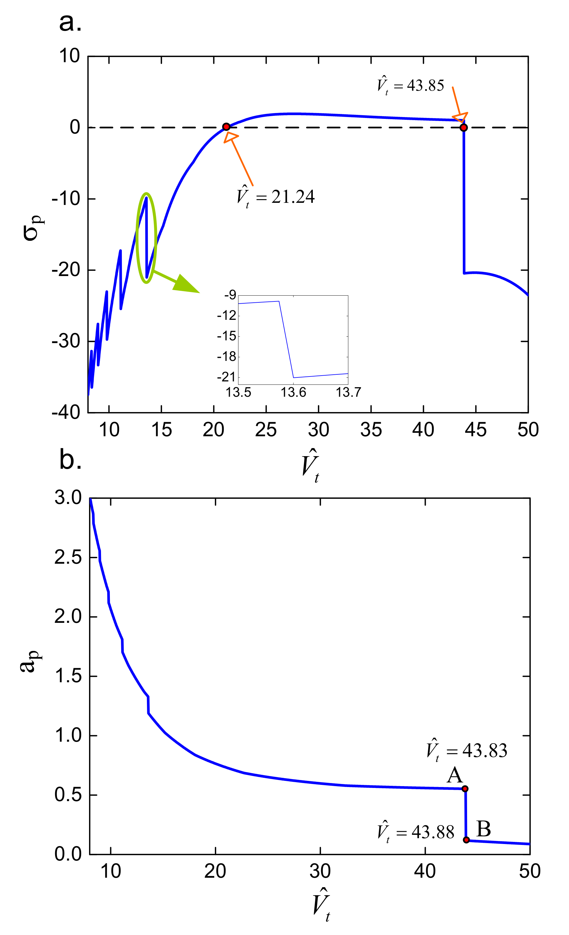
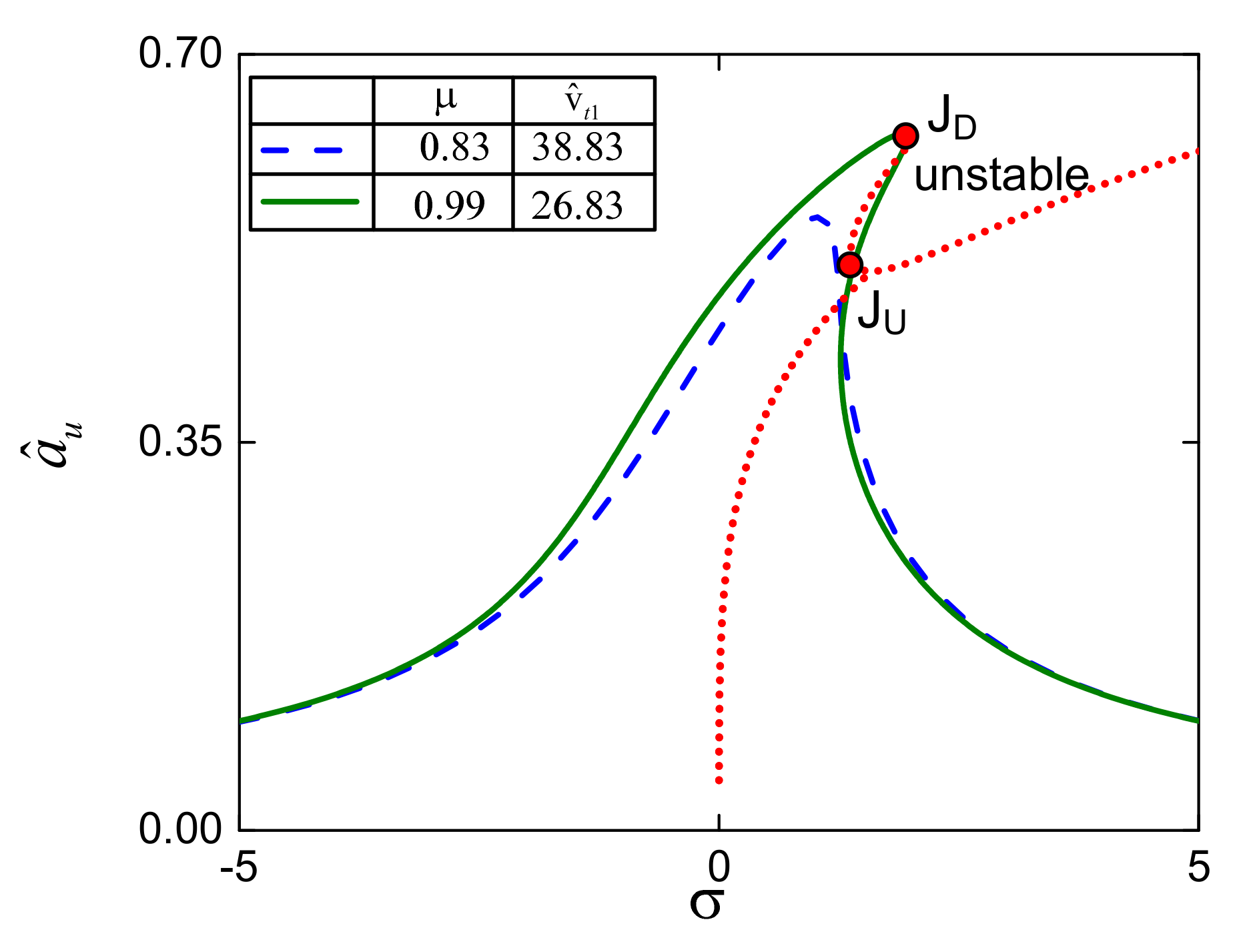
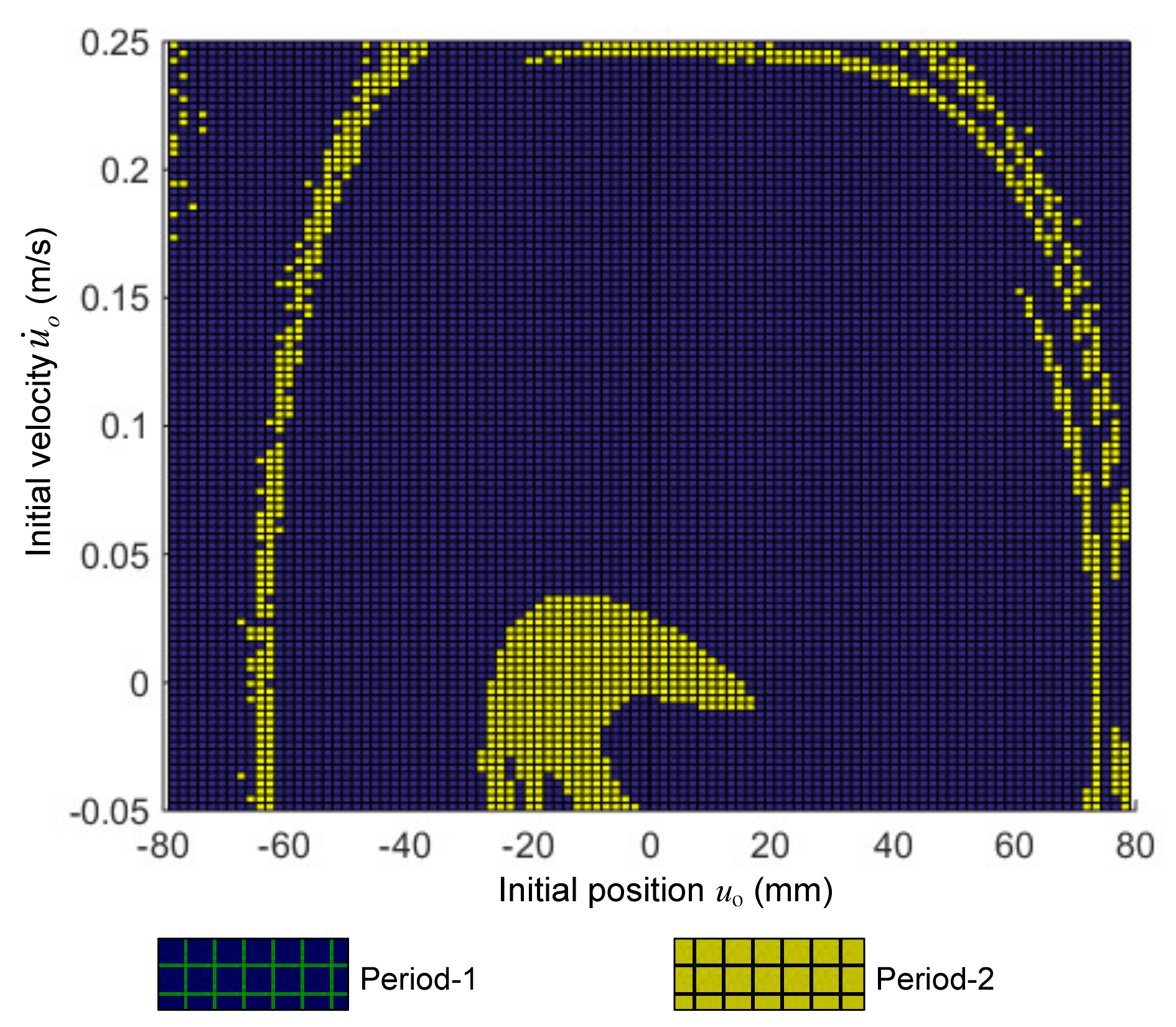
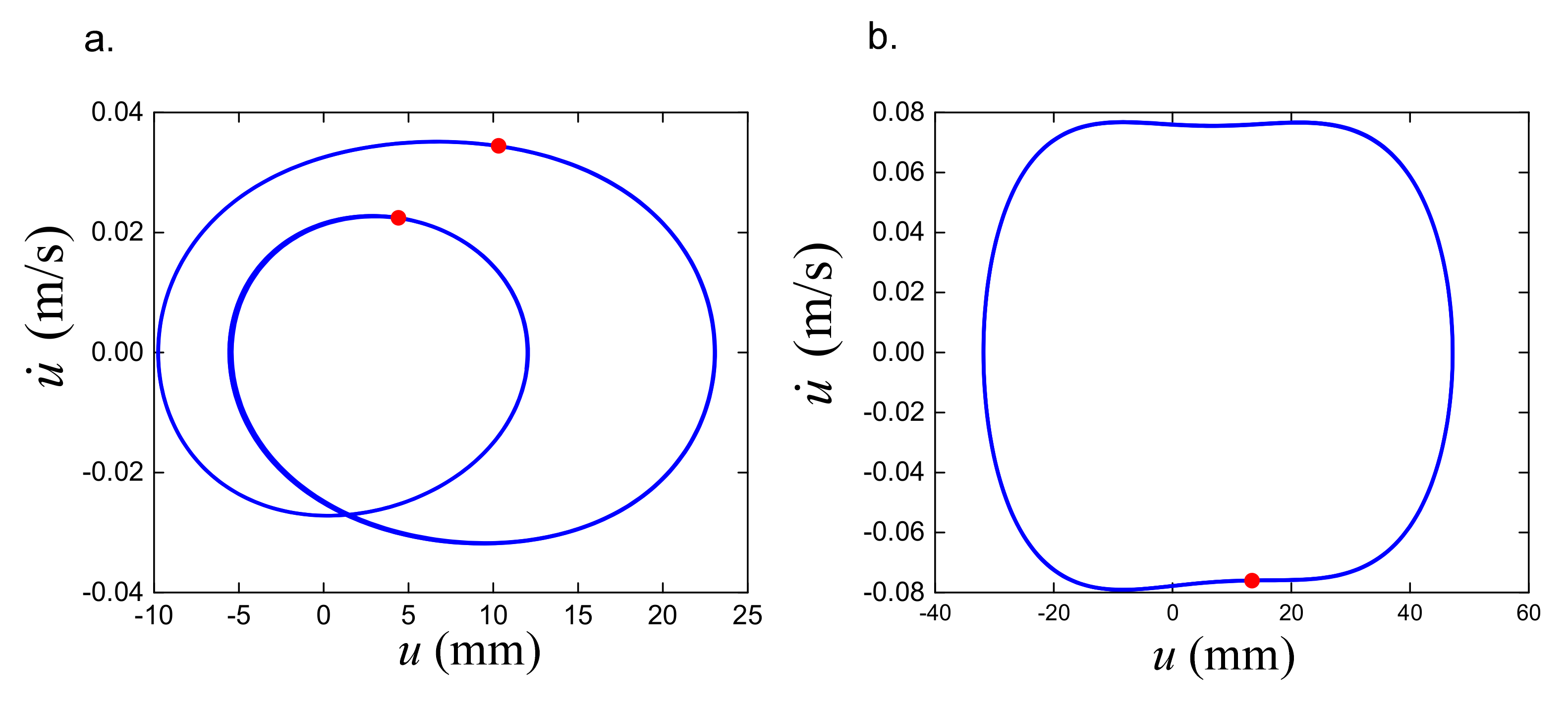
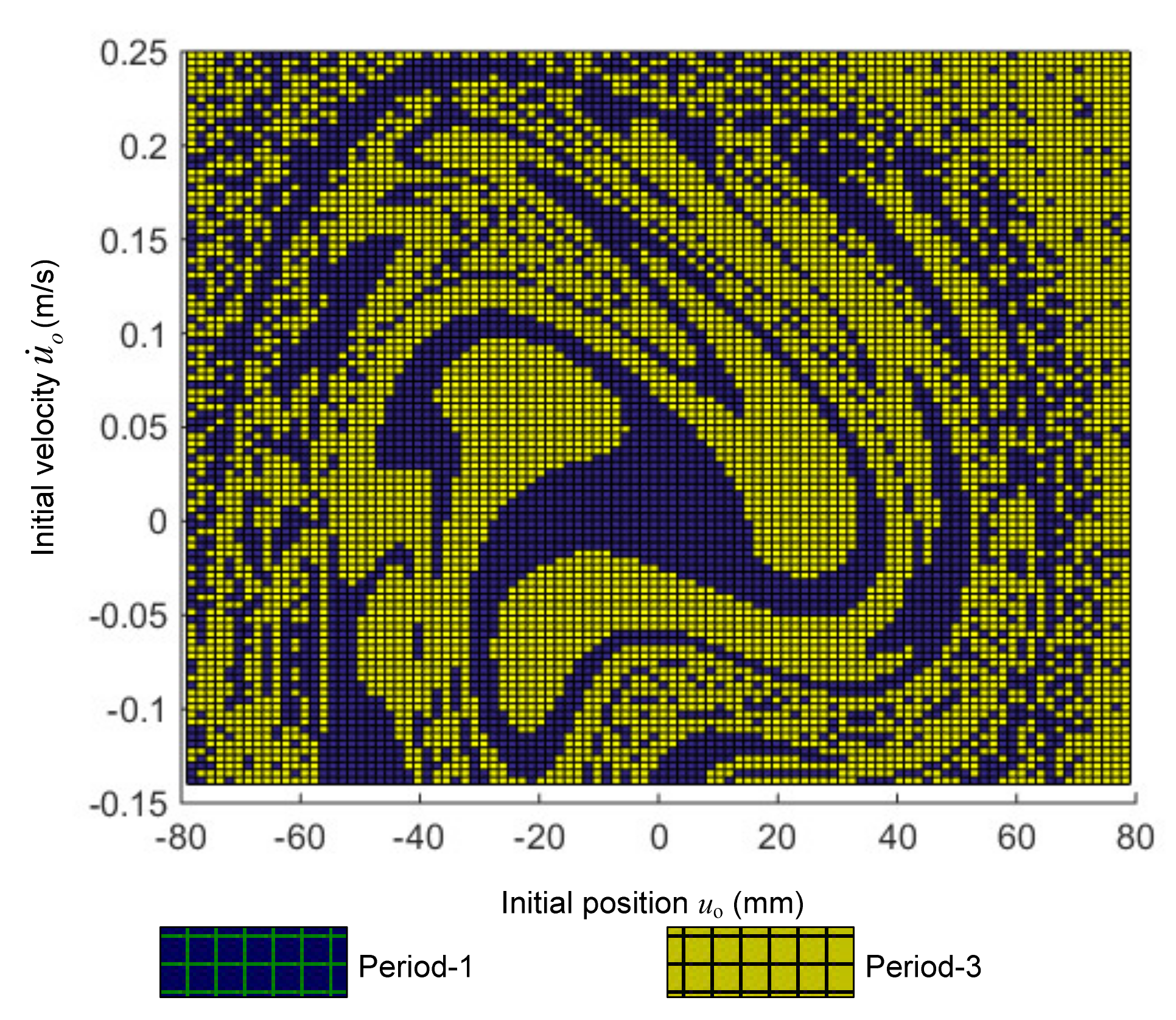
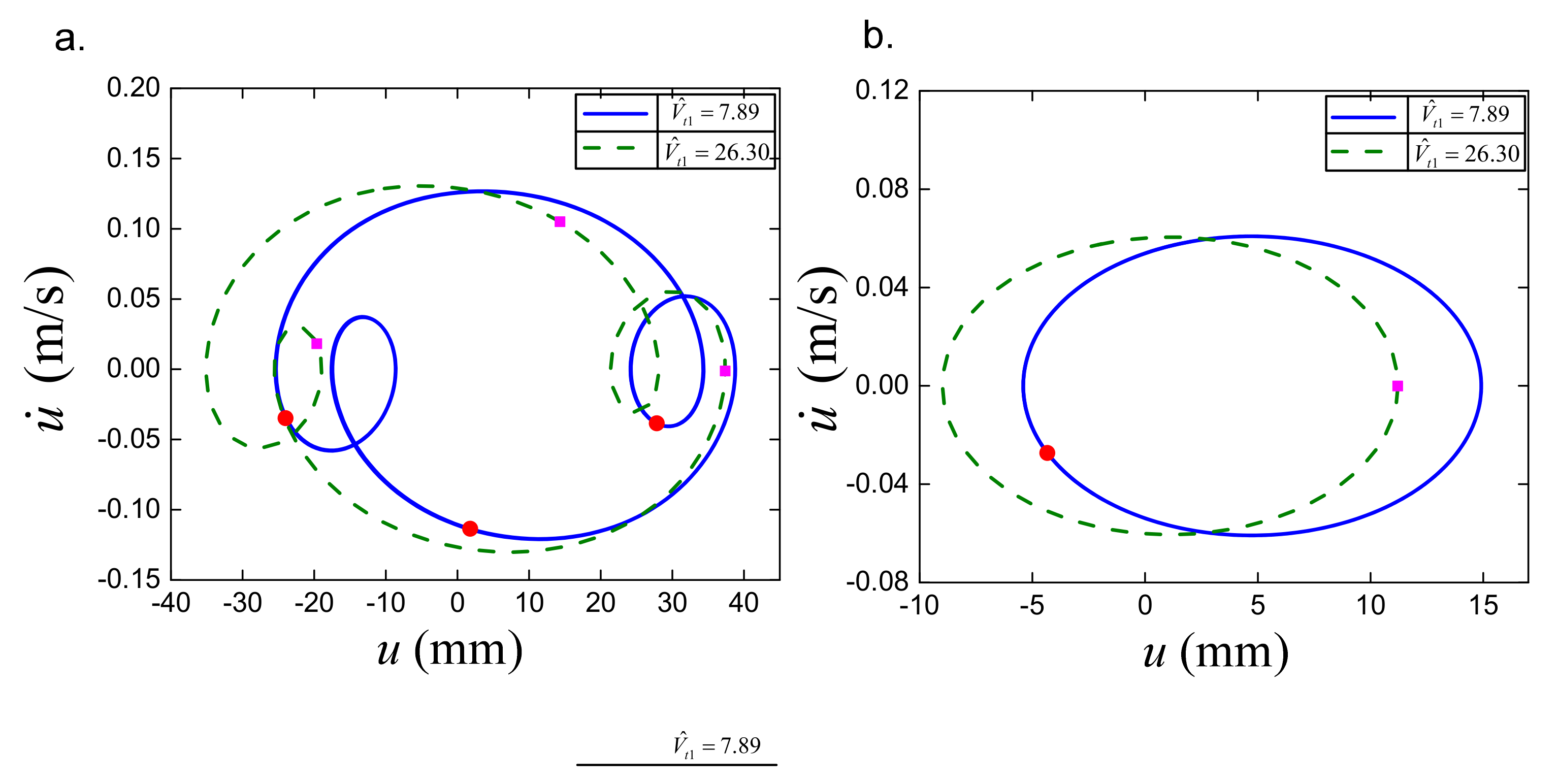
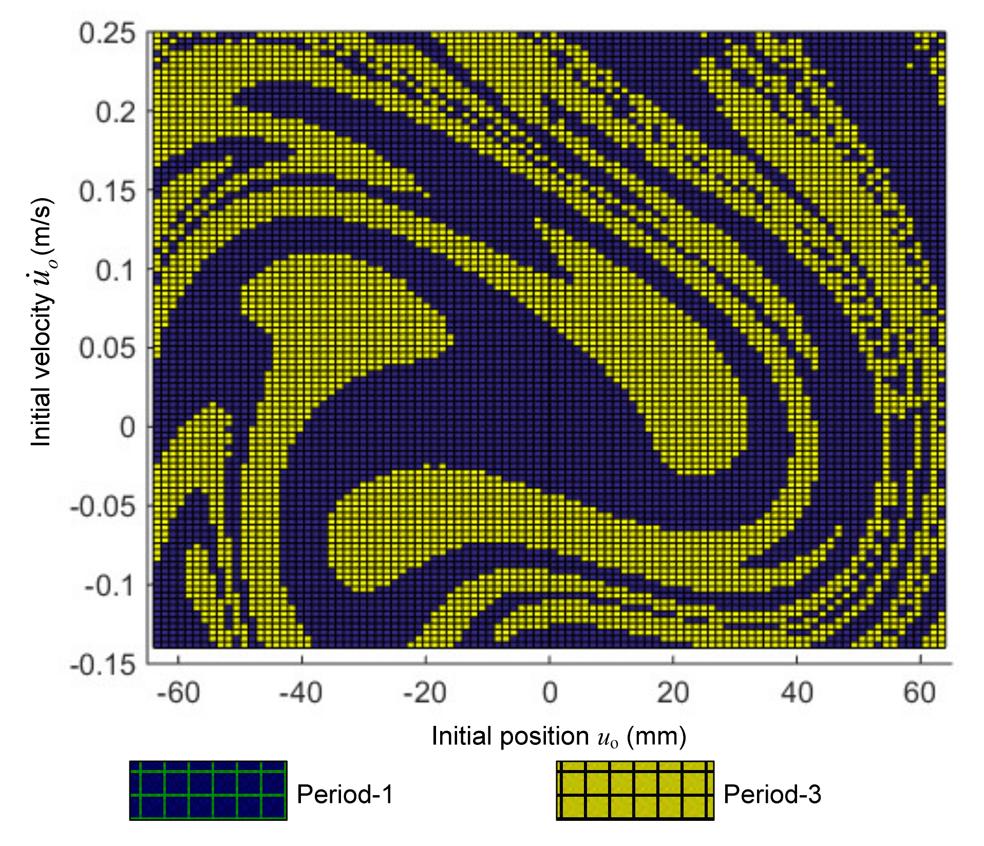
4.2. Complex Dynamic Response

Because of the nonlinear dynamic characteristic, as well as the existence of the relative sliding between the piston and cylinder, analyzing the complex behavior of the proposed system is needed. First of all, the sliding friction model (Fsf) given by Armstrong 1991 [34] is presented as the following:
F s f = F c + ( F s F c ) e ( v / v s ) n s + σ v
in which Fc is the Coulomb friction force, Fs is the static friction force, vs. is the Stribeck velocity, v is the relative velocity between two contacting surfaces, σ is the viscous friction coefficient, and ns is the exponent of the Stribeck curve.
In order to identify parameters of the friction model of a cylinder, instead of experimenting, a virtual model of a cylinder shown in Figure 17 is built through AMEsim software. This method ensures the accuracy and reduces the time because the environment of a virtual model is similar to an actual model. For instance, the heat exchange exists between the air in the cylinder and surrounding environment, the dead volume of the cylinder, frictional phenomenon, etc. Herein, the cylinder used for identification has the piston diameter of 80 mm, rod diameter of 32 mm, stroke length of 300 mm, and the dead volume at two ends of 50 cm3, whilst the parameters for simulation are given in Table 1. During the simulated process, the cylinder is fixed, meanwhile the speed of load attached at the end of the rod is controlled to track the constant value through introducing a PID controller. Simultaneously, its acceleration is measured by an accelerometer. In this identification, the frictional force between the cylinder and piston is not measured directly, and it is calculated as follows:
F s f = F 1 F 2 F e f   for   Extending F 2 F 1 F e f   for   Retracting  
In this calculation, due to constant velocity, the inertia force is ignored, Fef is the external force, F1 = P1A and F2 = P2(A − a) in which A, a are the areas of the piston and rod, P1 and P2 are the air pressure in chamber as denoted in Figure 17, which are measured by two pressure sensors.
Then, genetic algorithms, including three operations—reproduction, crossover, and mutation, as shown in Figure 18, are employed to determine optimal values of the friction model given in Equation (39). This work aims to minimize the cost function expressed by Equation (41). As observed in Figure 19, after 30 iterations, the cost function converges to zero.
J = 1 2 F m s f i F s f i 2
in which Fmsf is the friction force measured at ith constant velocity, and Fsf is the friction force calculated by Equation (40). The best values of the friction model are given in Table 2.
Figure 20 shows the friction force characteristic of the pneumatic cylinder model in which the solid line denotes the identified curve for extending stroke, whilst the reverse stroke, that is the retracting, is exhibited by the dashed line. It is noteworthy to see that the identified results match well with the simulated ones marked by the square and circle points according to the extending and retracting stroke, respectively. The friction force in the extending stroke is larger than the retracting one.
Accordingly, the dynamic equation of the system is rewritten as below:
M u ¨ + C u ˙ = 2 F s 2 F s f 1 s i g n ( u ˙ ) tan α + 2 F s f 2 s i g n ( u u ˙ ) u R + r 2 u 2 M g + F e cos ( ω t )
where Fsf1 and Fsf2 are calculated by Equation (39), and Fs is determined by Equation (1).
First of all, the amplitude–frequency curves obtained by multi-scale method and fourth-order Runge–Kutta algorithm are compared, as shown in Figure 21. Herein, the frequency of the excited force is swept up slowly from 0 to 10 Rad/s (denoted by the dashed line). In contract to slowly reducing the frequency of 10 Rad/s to 0, the amplitude–frequency curve is exhibited by the dot line. It can be seen that although the down jump point has a difference between two methods due to approximate error and exiting sliding friction between the piston and cylinder, two curves are still in good agreement.
Next, the complex behavior of the proposed system will be investigated through the numerical integration for Equation (42) using a fourth-order Runge–Kutta algorithm with various initial conditions, including velocity and position. The bifurcation diagram of Equation (42) for V ^ t = 7.89 , µ = 1.834, ω changed from 1 to 10 rad/s and the same other parameters as in Figure 8. The value of u ^ is determined by using Poincare map with the period T = 2π/ω. The simulated result is plotted in Figure 22, showing that if the initial condition is zero for both of the position and velocity, the dynamic response of the system (denoted by filled circles) will be period-2 oscillation as the excited frequency is within 2.2–2.6 rad/s. However, out of this range the solution is period-1 periodic. Meanwhile, the response marked by squares is realized by sweeping the parameter ω from 1 to 10 rad/s, for which the initial position and velocity are set at zero only for the first parameter ω and the final state of the system will be considered as the initial condition for the next value of ω. In this case, the oscillation transformed from period-1 to period-3 periodic occurred with ω around of 4 and 8 rad/s. Hence, it revealed from this figure that depending on the initial condition, the dynamic response of the system can be bifurcated at A (1.9 rad/s), B (2.8 rad/s), and C (4 rad/s), meaning that in the parameter ω < 1.9, only a period-1 solution exists, but 1.9 < ω < 2.8 two cases for two period-1 or period-2 solutions may appear. However, if the parameter is within B and C, there are two cases for period-1 periodic oscillation, and after C the dynamic behavior of the system can be a period-1 or period-3 solution.
Furthermore, in order to obtain the solution of the dynamic response, the family of the initial conditions named the attractor–basin phase portrait affecting on the dynamic response will be detected in the three cases following. In the first study case, the parameter ω is taken account into at value of 2.4 rad/s, while other parameters are simultaneously set as in Figure 22. As shown in Figure 22, it can be seen that the period-1 or period-2 solution may exist depending on the initial condition. It is interesting to see that in the attraction basin depicted in Figure 23, the attractor region of the period-1 oscillation is greater than that of the period-2 one. This means that the ability to obtain period-1 steady dynamic response is higher. Additionally, the vibration ability of the period-1 oscillation plotted in Figure 24b is higher than that of period-2 one depicted in Figure 24a, in which the initial position and velocity of the first solution is zero but the second one is obtained for u o = 20   mm   and   u ˙ o =   0.2   m / s , meanwhile, the fixed points calculated by Poincare section are annotated by filled circles.
In the second study case, suppose that ω = 6 rad/s and other parameters are not changed. In this case, the dynamic response of the QZSPVI can be period-1 or period-3 solution. As depicted in Figure 25, the possibility of appearing in the period-1 steady response is reduced because the region of attractors for which the period-1 solution occurred is narrower than that in the first case. Furthermore, in this case as shown in Figure 26 (the detailed annotation of line types is presented in right-top corner panel of each figure), the vibration level of the period-1 solution (Figure 26b) is lower than that of the period-3 one (Figure 26a). Both solutions also revealed that the vibration of the system occurs at a position which drifted away from the equilibrium position (u = 0).
In the third study case, the dimensionless volume of the auxiliary tank is increased to the value of 26.30, but other parameters and frequency are the same as in the second case. To guarantee that the minimum stiffness is nearly zero, the pressure ratio is calculated at a value of 0.997. The result is that the area of the period-1 solution is expanded compared with the second case, as shown in Figure 27. Similar to the second case, the amplitude and velocity of the period-1 solution are reduced compared with the period-3 oscillation as shown in Figure 26 in which the phase orbits are drawn by the dashed line. Meanwhile, the fixed point is annotated by squares. This case confirms that the position at which the load plate oscillates around was moved to the equilibrium position.

5. Conclusions

A pneumatic vibration isolation model with quasi-zero stiffness characteristic was studied and analyzed in this paper. The dynamic stiffness of the QZSPVI was determined and numerically calculated. Analysis results indicated that the stiffness curve is asymmetrical around the equilibrium position and its asymmetry may be reduced according to the increase in the volume of the auxiliary tank. The condition for which the minimum stiffness obtains quasi-zero value was analyzed. Besides, the expected working region in which the pressure in the stiffness correction mechanism is always positive was obtained. The spring force curve was approximated through expanding Taylor series to order-5. By using multi-scale methods, the force transmissibility of the QZSPVI was then analyzed in detail, showing that the transmitted curve may be bent to the left or the right depending on the auxiliary tank volume and the pressure ratio. Furthermore, the stability of the analysis response was also studied.
In addition, parameter bifurcation analysis of the QZSPVI had been realized through numerical integration from the original dynamic equation. Simultaneously, fixed points had been also calculated by using a Poincare map. The result proved that the system could occur in period-1, period-2, or period-3 of oscillation depending on the initial conditions. Under given excited frequencies, the attractor–basin phase portrait had been detected.
From these analysis results, we confirmed that the lower the stiffness, the larger the isolation region toward the low frequency. The bigger the volume of the tank is, the higher isolation effectiveness is. Additionally, the basin of initial conditions to occur in the non-resonance solution is extended according to reduction in the stiffness. This model can be applied effectively in the field of low frequency vibration isolation system, having a high isolated load such as platform for vibration sensitive instruments, an isolated seat for vehicles, mount of engine, and so forth.

Author Contributions

Conceptualization, N.Y.P.V.; methodology, T.D.L. and N.Y.P.V.; software, N.Y.P.V.; validation, N.Y.P.V.; formal analysis, N.Y.P.V.; investigation, T.D.L.; resources, N.Y.P.V.; data curation, T.D.L.; writing—original draft preparation, T.D.L. and N.Y.P.V.; writing—review and editing, T.D.L.; visualization, T.D.L. and N.Y.P.V.; supervision, T.D.L. and N.Y.P.V. All authors have read and agreed to the published version of the manuscript.

Funding

This research is funded by Vietnam National Foundation for Science and Technology Development (NAFOSTED) under grant number 107.01-2020.36.

Conflicts of Interest

The authors declare no conflict of interest.

References

  1. Zhang, Z.; Peng, H.; Yan, J. Micro-cutting characteristics of EDM fabricated high-precision polycrystalline diamond tools. Int. J. Mach. Tool Manuf. 2013, 65, 99–106. [Google Scholar] [CrossRef]
  2. Song, J.; Pan, W.; Wang, K.; Chen, F.; Sun, Y. Fabrication of micro-reentrant structures by liquid/gas interface shape-regulated electrochemical deposition. Int. J. Mach. Tool Manuf. 2020, 10, 99–106. [Google Scholar] [CrossRef]
  3. Liu, C.; Yu, K. Accurate modeling and analysis of a typical nonlinear vibration isolator with quasi-zero stiffness. Nonlinear Dyn. 2020, 100, 2141–2165. [Google Scholar] [CrossRef]
  4. Wang, K.; Zhou, J.; Chang, Y.; Ouyang, H.; Xu, D.; Yang, Y. A nonlinear ultra-low-frequency vibration isolator with dual quasi-zero-stiffness mechanism. Nonlinear Dyn. 2020, 101, 755–773. [Google Scholar] [CrossRef]
  5. Xu, D.; Zhang, Y.; Zhou, J. On the analytical and experimental assessment of the performance of a quasi-zero-stiffness isolator. J. Vib. Control 2013, 20, 2314–2325. [Google Scholar] [CrossRef]
  6. Le, T.D.; Ahn, K.K. Experimental investigation of a vibration isolation system using negative stiffness structure. Int. J. Mech. Sci. 2013, 70, 99–112. [Google Scholar] [CrossRef]
  7. Zhou, J.; Wang, X.; Xu, D.; Bishop, S. Nonlinear dynamic characteristics of a quasi-zero stiffness vibration isolator with cam-roller- spring mechanism. J. Sound Vib. 2015, 346, 53–69. [Google Scholar] [CrossRef]
  8. Lan, C.C.; Yang, S.A.; Wu, Y.S. Design and experiment of a compact quasi-zero-stiffness isolator capable of wide range of loads. J. Sound Vib. 2014, 333, 4843–4858. [Google Scholar] [CrossRef]
  9. Sun, X.; Jing, X. Multi-direction vibration isolation with quasi-zero stiffness by employing geometrical nonlinearity. Mech. Syst. Signal Process. 2015, 62, 149–163. [Google Scholar] [CrossRef]
  10. Hao, Z.; Cao, Q. The isolation characteristics of an archetypal dynamical model with stable-quasi-zero-stiffness. J. Sound Vib. 2015, 340, 61–79. [Google Scholar] [CrossRef]
  11. Chai, K.; Yang, Q.C.; Lou, J.J. Dynamic characteristic analysis of two-stage quasi-zero stiffness vibration isolation system. J. Vibroengineering 2016, 10, 22–27. [Google Scholar]
  12. Ding, H.; Ji, J.; Chen, L.Q. Nonlinear vibration isolation for fluid-conveying pipues using quasi-zero stiffness characteristics. J. Mech. Syst. Signal Process. 2019, 121, 675–688. [Google Scholar] [CrossRef]
  13. Gatti, G. Statics and dynamics of a nonlinear oscillator with quasi-zero stiffness behaviour for large deflections. Commun. Nonlinear Sci. Numer. Simul. 2019, 83, 105143. [Google Scholar] [CrossRef]
  14. Bian, J.; Jing, X. Analysis and design of a novel and compact X-structured vibration isolation mount (X-Mount) with wider quasi-zerostiffness range. Nonlinear Dyn. 2020, 101, 2195–2222. [Google Scholar] [CrossRef]
  15. Gatti, G. Optimizing elastic potential energy via geometric nonlinear stiffness. Commun. Nonlinear Sci. Numer. Simul. 2021, 103, 106035. [Google Scholar] [CrossRef]
  16. Yan, G.; Zou, H.X.; Wang, S.; Zhao, L.C.; Wu, Z.Y.; Zhang, W.M. Bio-inspired vibration isolation: Methodology and design. Appl. Mech. Rev. 2021, 73, 020801. [Google Scholar] [CrossRef]
  17. Le, T.D.; Nguyen, V.A.D. Low frequency vibration isolator with adjustable configurative parameter. Int. J. Mech. Sci. 2017, 134, 224–233. [Google Scholar] [CrossRef]
  18. Zheng, Y.; Li, Q.; Yan, B.; Luo, Y.; Zhang, X. A Stewart isolator with high-static-low-dynamic stiffness struts based on negative stiffness magnetic springs. J. Sound Vib. 2014, 422, 390–408. [Google Scholar] [CrossRef]
  19. Zheng, Y.; Zhang, X.; Lue, Y.; Yan, B.; Ma, C. Design and experiment of a high-static-low-dynamic stiffness isolator using a negative stiffness magnetic spring. J. Sound Vib. 2016, 360, 31–52. [Google Scholar] [CrossRef]
  20. Zhang, F.; Shao, S.; Tian, Z.; Xu, M.; Xie, M. Active passive hybrid vibration isolation with magnetic negative stiffness isolator based on Maxwell normal stress. Mech. Syst. Signal Process. 2019, 123, 244–263. [Google Scholar] [CrossRef]
  21. Dong, G.; Zhang, X.; Luo, Y.; Zhang, Y.; Xie, S. Analytical study of the low frequency multi-direction isolator with high-static-low-dynamic stiffness struts and spatial pendulum. Mech. Syst. Signal Process. 2018, 110, 521–539. [Google Scholar] [CrossRef]
  22. Zhao, Y.; Cui, J.; Zhao, J.; Bian, X.; Zou, L. Improving low frequency isolation performance of optical platforms using electromagnetic active-negative-stiffness method. Appl. Sci. 2020, 10, 7342. [Google Scholar] [CrossRef]
  23. Yuan, S.; Sun, Y.; Zhao, J.; Meng, K.; Wang, W.; Pu, H.; Peng, Y.; Luo, J.; Xie, S. A tunable quasi-zero stiffness isolator based on a linear electromagnetic spring. J. Sound Vib. 2020, 482, 115449. [Google Scholar] [CrossRef]
  24. Erin, B.; Wilso, B.; Zapfe, J. An improved model of a pneumatic vibration isolator: Theory and experiment. J. Sound Vib. 1998, 218, 81–101. [Google Scholar] [CrossRef]
  25. Lee, J.H.; Kim, K.J. Modelling of nonlinear complex stiffness of dual-chamber pneumatic spring for precision vibration isolators. J. Sound Vib. 2007, 301, 909–926. [Google Scholar] [CrossRef]
  26. Mankovits, T.; Szabó, T. Finite element analysis of rubber bumper used in air-springs. Procedia Eng. 2012, 48, 388–395. [Google Scholar] [CrossRef] [Green Version]
  27. Danh, L.T.; Ahn, K.K. Active pneumatic vibration isolation system using negative stiffness structures for a vehicle seat. J. Sound Vib. 2014, 333, 1245–1268. [Google Scholar] [CrossRef]
  28. Le, T.D.; Bui, M.T.N.; Ahn, K.K. Improvement of vibration isolation performance of isolation system using negative stiffness structure. IEEE/ASME Trans. Mechatron. 2016, 21, 1561–1571. [Google Scholar] [CrossRef]
  29. Palomares, E.; Nieto, A.J.; Morales, A.L.; Chicharro, J.M.; Pintado, P. Numerical and experimental analysis of a vibration isolator equipped with a negative stiffness system. J. Sound Vib. 2018, 414, 31–42. [Google Scholar] [CrossRef]
  30. Nguyen, C.H.; Ho, C.M.; Ahn, K.K. An air spring vibration isolator based on a negative stiffness structure for vehicle seat. Appl. Sci. 2021, 11, 11539. [Google Scholar] [CrossRef]
  31. Vo, N.Y.P.; Le, T.D. Static analysis of low frequency isolation model using pneumatic cylinder with auxiliary chamber. Int. J. Precis. Eng. Manuf. 2020, 21, 681–697. [Google Scholar] [CrossRef]
  32. Yin, Y.; Sun, B.; Han, F. Self-locking avoidance and stiffness compensation of a three-axis micromachined electrostatically suspended accelerometer. Sensors 2016, 16, 711. [Google Scholar] [CrossRef] [PubMed] [Green Version]
  33. Gatt1, G.; Shaw, A.D.; Goncalves, P.J.P.; Brennan, M.J. On the detailed design of a quasi-zero stiffness device to assist in the realisation of a translational Lanchester damper. Mech. Syst. Signal Process. 2022, 16, 108258. [Google Scholar] [CrossRef]
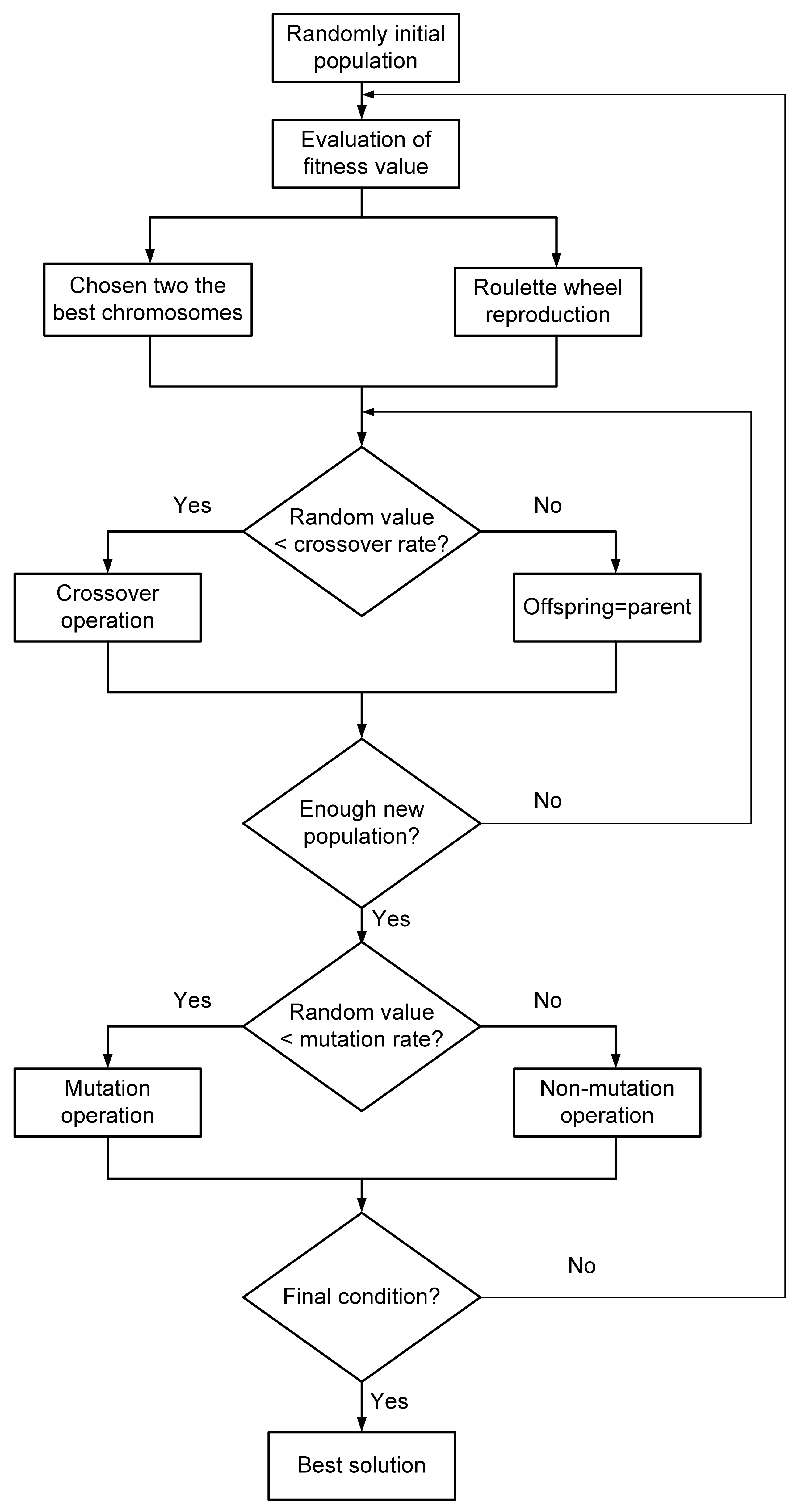
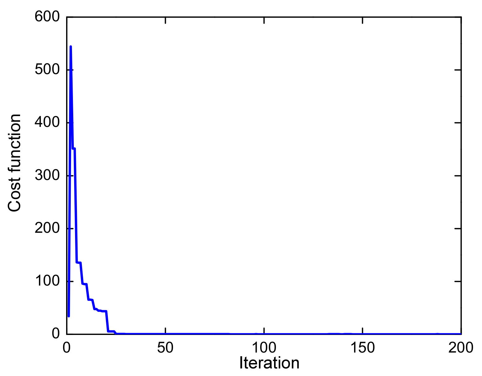
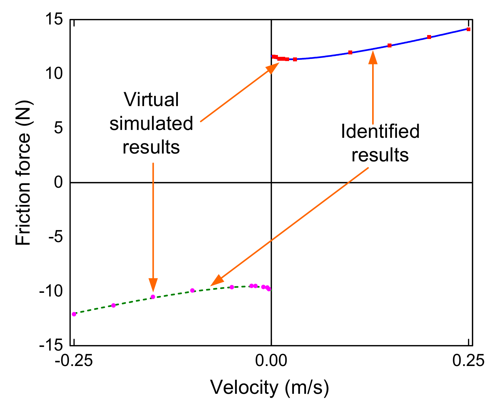
  34. Tran, X.B.; Nguyen, V.L.; Tran, K.D. Effects of friction models on simulation of pneumatic cylinder. Mech. Sci. 2019, 10, 517–528. [Google Scholar] [CrossRef]
Figure 1. (a) Schematic diagram of the QZSPVI composed by the LBM and SCM, (b) Specific states of the QZSPVI.
Applsci 12 02378 g001
Figure 2. (a) The relationship between the initial volume and pressure in cylinder 1 for Ho = 73.5 mm and A1 = 0.0095 m2. (b) Effect of the initial pressure Pso1 on the isolated mass and Vt = 0.01 m3, (c) Effect of tank volume Vt of the isolated mass and Pso1 = 2 bar.
Applsci 12 02378 g002
Figure 3. (a) Comparison between of the original (solid line) and 5th order approximated (dot line) curve of the elastic force; (b) The error percentage between the exact solution and approximation one.
Applsci 12 02378 g003
Figure 4. (a) The vertical stiffness surface in the space V ^ t , u ^ , K ^ s for pressure ratio µ = 1.83; (b) The dynamic stiffness curves for different values of dimensionless tank volume given in the right top corner panel.
Applsci 12 02378 g004
Figure 5. The influence of auxiliary tank volume V ^ t on the minimum stiffness position.
Applsci 12 02378 g005
Figure 6. (a). The quasi-zero stiffness surface in the space ( V ^ t , u ^ , μ ); (b). The pressure ratio curve for various values of V ^ t ; (c). Slope of stiffness curve in dimensionless form.
Applsci 12 02378 g006
Figure 7. Stiffness curve for different values of µ given in the panel of figure: (a) Quasi-zero stiffness at position u ^ = 0.008 ;   0.021 ;   0.046 ;   0.083 ; (b) Arbitrary stiffness.
Applsci 12 02378 g007
Figure 8. The stiffness curve of the QZSPVI for ξ = 0.1 ;   A ^ = 0.16 ;   V ^ t = 13.153 ;   H ^ o = 0.53 , Pe1 = 1.85 bar, and different values of µ.
Applsci 12 02378 g008
Figure 9. Force transmissibility of the QZSPVI for various values of µ and the same other parameters as in Figure 8 (the details of types of lines are presented in panel).
Applsci 12 02378 g009
Figure 10. Comparing force transmissibility of the QZSPVI and EPVI for various values of µ and the same other parameters as in Figure 8 (the details of types of lines are presented in panel).
Applsci 12 02378 g010
Figure 11. Effect of the pressure ratio on the peak frequency σp of the QZSPVI for the same parameters as in Figure 8.
Applsci 12 02378 g011
Figure 12. The relation of pressure ratio versus the auxiliary tank volume, the same other parameters as in the first case.
Applsci 12 02378 g012
Figure 13. The dynamic stiffness curve of the QZSPVI for the different values of the auxiliary tank volume as annotated in Figure. Meanwhile, the pressure ratio is calculated as in Figure 9.
Applsci 12 02378 g013
Figure 14. The peak frequency curve (a) and peak amplitude curve (b) of the QZSPVI for the same parameters as in Figure 13.
Applsci 12 02378 g014
Figure 15. Force transmissibility of the QZSPVI for various values of V ^ t including 7.89; 14.46, 18.41, 24.99, 39.45, and the same other parameters as in Figure 14 (The annotation of line types indicated in panel of figure).
Applsci 12 02378 g015
Figure 16. The stability of the response curve.
Applsci 12 02378 g016
Figure 17. Virtual test-rig of pneumatic cylinder.
Applsci 12 02378 g017
Figure 18. Low chart of the genetic algorithm.
Applsci 12 02378 g018
Figure 19. The value of cost function with respect to iteration.
Applsci 12 02378 g019
Figure 20. Steady-state friction force characteristic.
Applsci 12 02378 g020
Figure 21. Multi-scale method compared with numerical integration.
Applsci 12 02378 g021
Figure 22. Bifurcation diagram of Equation (42) for V ^ t = 7.89 , µ = 1.834, ω changed from 1 to 10 rad/s and the same.
Applsci 12 02378 g022
Figure 23. Attractor–basin phase portrait for ω = 2.4 rad/s, other parameters set as in Figure 22.
Applsci 12 02378 g023
Figure 24. Phase orbit of Equation (42) for ω = 2.4 rad/s and u o = 0   and   u ˙ o = 0 (a) u o = 20   mm   and   u ˙ o = 0.2   m / s (b).
Applsci 12 02378 g024
Figure 25. Attraction basin for ω = 6 rad/s and the same for other parameters as in Figure 22.
Applsci 12 02378 g025
Figure 26. The phase orbits of the system for V ^ t = 7.89 ;   26.30 and u o = 20   mm   and   u ˙ o = 0.05   m / s (a); u o = 0   and   u ˙ o = 0 (b).
Applsci 12 02378 g026
Figure 27. Attraction basin for ω = 6rad/s, µ = 0.997, and V ^ t = 26.30 , the same other parameters as in Figure 22.
Applsci 12 02378 g027
Table 1. Parameters for simulation.
ParameterOriginal Value
Atmosphere pressure1 bar
Specific heat ratio1.4
Thermal exchange coefficient500 J/mm2/K/s
External temperature293.15 K
External force100 N
Source pressure5 bar
Velocity of load0.003; 0.006; 0.01; 0.015; 0.02; 0.03; 0.05; 0.1; 0.15; 0.2; 0.25 m/s
Table 2. Values of friction force model.
ParameterExtendingRetracting
Fc4.338−3.904
Fs11.655−9.906
vs0.4961−0.372
σ23.723.356
n0.6810.681
Publisher’s Note: MDPI stays neutral with regard to jurisdictional claims in published maps and institutional affiliations.

