Local Path-Planning Simulation and Driving Test of Electric Unmanned Ground Vehicles for Cooperative Mission with Unmanned Aerial Vehicles

Featured Application

Local path-planning simulation and experiment using potential field considering calculation time.

Abstract

Recently, various studies related to the development of unmanned vehicles have been conducted around the world. In particular, unmanned ground vehicles (UGVs) and unmanned aerial vehicles (UAVs) have been developed and utilized for various purposes. In this study, we developed a method for the path generation of UGVs in a system in which one operator controls many different types of unmanned vehicles. In the driving control system (DCS), it is necessary to process sensor data such as GPS/INS and LiDAR when generating a path by receiving the target waypoint from the ground control station. In addition, the DCS must upload the current location, posture, state, etc., as well as save driving log. Therefore, in order to recognize obstacles in real time and generate a path, a safe path generation algorithm with a short computation time is required. Among the various path generation methods, the potential field algorithm was selected, and the algorithm was modified to reduce the computation time. The computation time before and after modification of the algorithm was obtained and compared through simulation, and the algorithm was verified through application to an actual system by performing an obstacle avoidance experiment and a simultaneous control experiment for two UGVs.

1. Introduction

The interest in and demand for unmanned vehicles that perform unmanned missions have continuously increased; in particular, UAV (unmanned aerial vehicle)-related technologies are being developed rapidly. However, UAVs have limitations such as short operating time and small payload, making it difficult to mount various equipment and to acquire data near the ground. If UGVs (unmanned ground vehicles) perform missions together, more diverse missions can be performed more efficiently. Such research is actively underway worldwide. Cantelli [1] tried to create a UGV route more precisely using UAV images, while Grocholsky [2] developed a system for local search simultaneously using both UAVs and UGVs. In addition, in order to overcome the short operation time of UAVs, Mathew [3] studied an operation method considering charging, while Ropero [4] studied how to optimize the UAV’s path for charging.

Since this study is one in which one operator simultaneously operates multiple UAVs and UGVs, the operator cannot be in the field where the UGVs and UAVs operate. Therefore, the UGVs are controlled remotely, and an autonomous driving function must be implemented because one person cannot directly control multiple unmanned vehicles at the same time.

Autonomous driving is being actively researched by numerous companies, universities, and research institutes around the world. Overcoming the uncertainty encountered while driving is the key, and, for this purpose, autonomous driving consists of environmental awareness, path planning, and driving control [5]. Environment recognition is a technology that recognizes the surrounding environment for autonomous driving, and cameras and LiDAR are often used as sensors. Path-planning methods are classified into graph-search-based, sampling-based, interpolation-based, and optimization-based methods [5], whereby a path that can be safely driven is created using environmental awareness information.

Graph-search-based methods find a path by creating a number of nodes within the domain and composing it as a graph [6], including methods such as the Dijkstra [7] algorithm that finds the shortest path and the A-Star [8] algorithm that finds the optimal path using a heuristic method. Sampling-based methods randomly sample and connect to the surrounding space [9], including methods such as the probabilistic roadmap method [10] and rapidly explored random tree [11]. Interpolation-based methods define a function with multiple coefficients and find the coefficients [12]. Optimization-based methods formulate an optimization problem consisting of constraints and cost functions, thereby finding a path that minimizes the cost function, including methods such as the potential field algorithm [7,8] and model predictive control (e.g., [13]).

The potential field method is broadly applied for real-time collision-free path planning [14]. In this method, an attractive force is generated in the goal direction, and a repulsive force is generated from an obstacle. Although the potential field algorithm is often used because it is mathematically simple, problems such as a local minimum and vibration around obstacles occur [14]. Sfeir [15] proposed new formulas for reducing oscillations and avoiding conflicts when obstacles are located near a target. Kim [16,17] proposed a new framework to escape from the local minimum of a robot path using the potential field method.

Many studies have tried to apply path-planning algorithms in real time [18,19]; although the potential field method is relatively efficient, it still requires substantial effort to use it in real time. In this study, an environmental recognition and control system for autonomous driving was configured in a UGV driven based on a GPS target point to perform a ground–aerial cooperative mission, and local path planning was performed by applying the potential field algorithm as an optimization-based method. In the developed UGV, GPS/INS processing, LiDAR processing, path planning, and driving log storage had to all be performed by one controller; therefore, a path-planning algorithm that could be operated in real time had to be implemented. Although the potential field algorithm is efficient, the calculation time is insufficient; hence, it was modified to enable faster operation. It was confirmed through simulation that the generated path was not significantly different from that obtained by the existing method. Furthermore, an obstacle avoidance experiment and an experiment in which one operator simultaneously operates three UAVs and two UGVs were conducted to confirm that the modified potential field algorithm can be used in practice.

2. UGV System Configuration

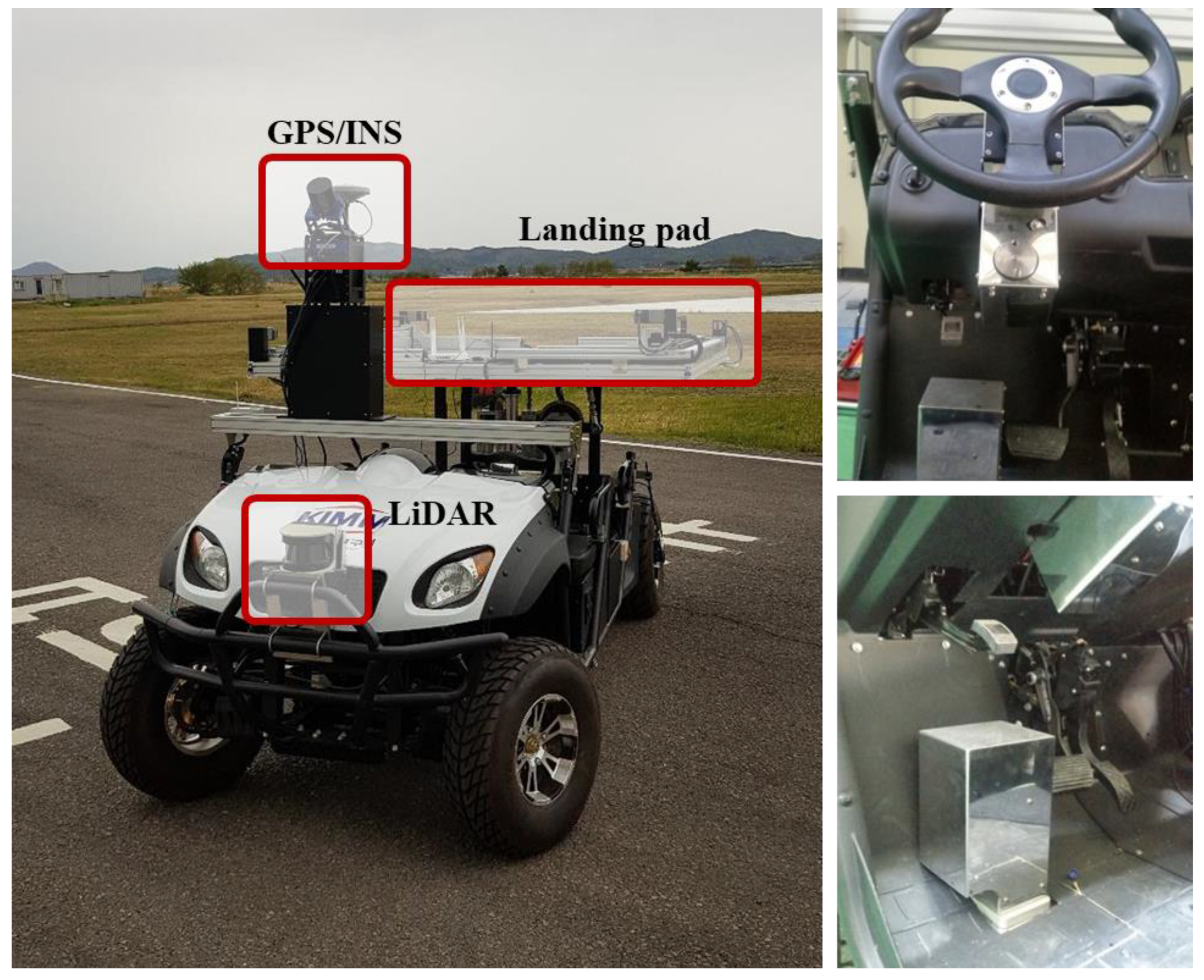
As shown in Figure 1, the developed UGV was equipped with a landing pad (UAV interface system) for takeoff and landing of UAVs, while a 2D LiDAR sensor was installed in the front part for recognizing obstacles. The top of the UGV was equipped with GPS/INS sensors and a mapping system [20] for cooperative missions with UAVs.

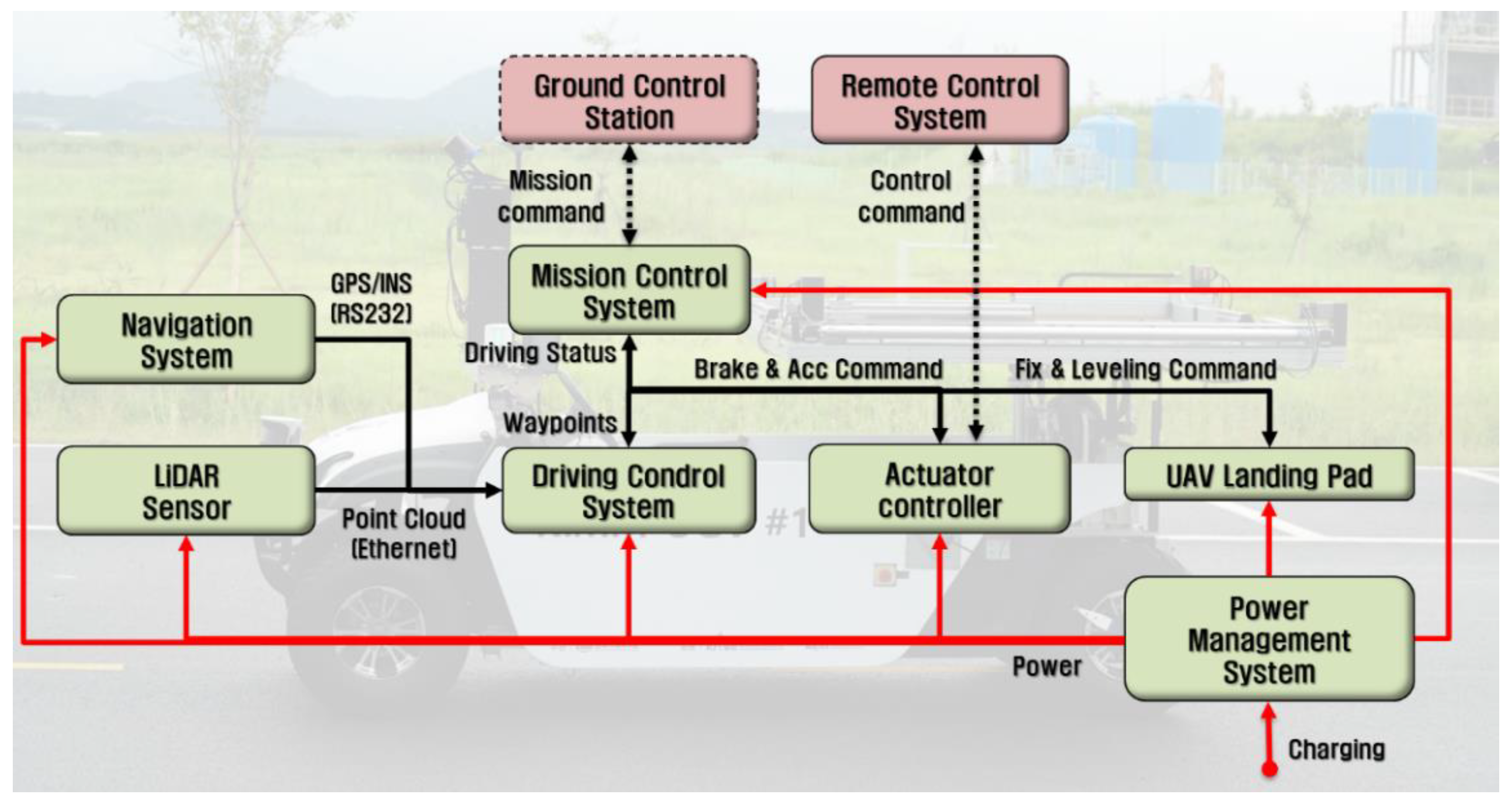
The configuration of the system is shown in Figure 2. The mission control system (MCS) was developed using a TI micro controller (TMS320F28335) and equipped with a modem to communicate with the control station, as well as transmit/receive data through RS232. It receives the UGV operation mode and target points from the control station, and it sends the vehicle’s location, direction, and battery status. In addition, it transmits commands and information through CAN communication with the internal driving control system (DCS) and UAV landing pad controller.

Adventech’s industrial PC UNO-3284G was used as the DCS; it receives and processes data from the navigation sensors and LiDAR, and it generates a local path to avoid obstacles by receiving target points from the MCS. The generated local path is transmitted to the MCS capable of real-time control, and the steering angle and pedal control amount are calculated.

The actuator controller receives the steering angle and acceleration/brake pedal input from the MCS to control the actuators mounted on the UGV. The steering angle is received in the form of an angle, and the pedal input is received as a percentage; it is controlled to generate a constant torque until it reaches the target value within a certain range.

Trimble’s Applanix AP-20E GPS/INS was used as a navigation sensor, and Sick’s LMS511 was used for LiDAR. The LiDAR is connected with the DCS via Ethernet, while the GPS/INS is connected with the DCS via RS232.

The UAV landing pad is equipped with an IMU, actuators, and controllers to keep the UAV level when landing, as well as a mechanism for fixing the UAV so that it can travel in the landed state.

3. Path Planning

3.1. Potential Field Algorithm

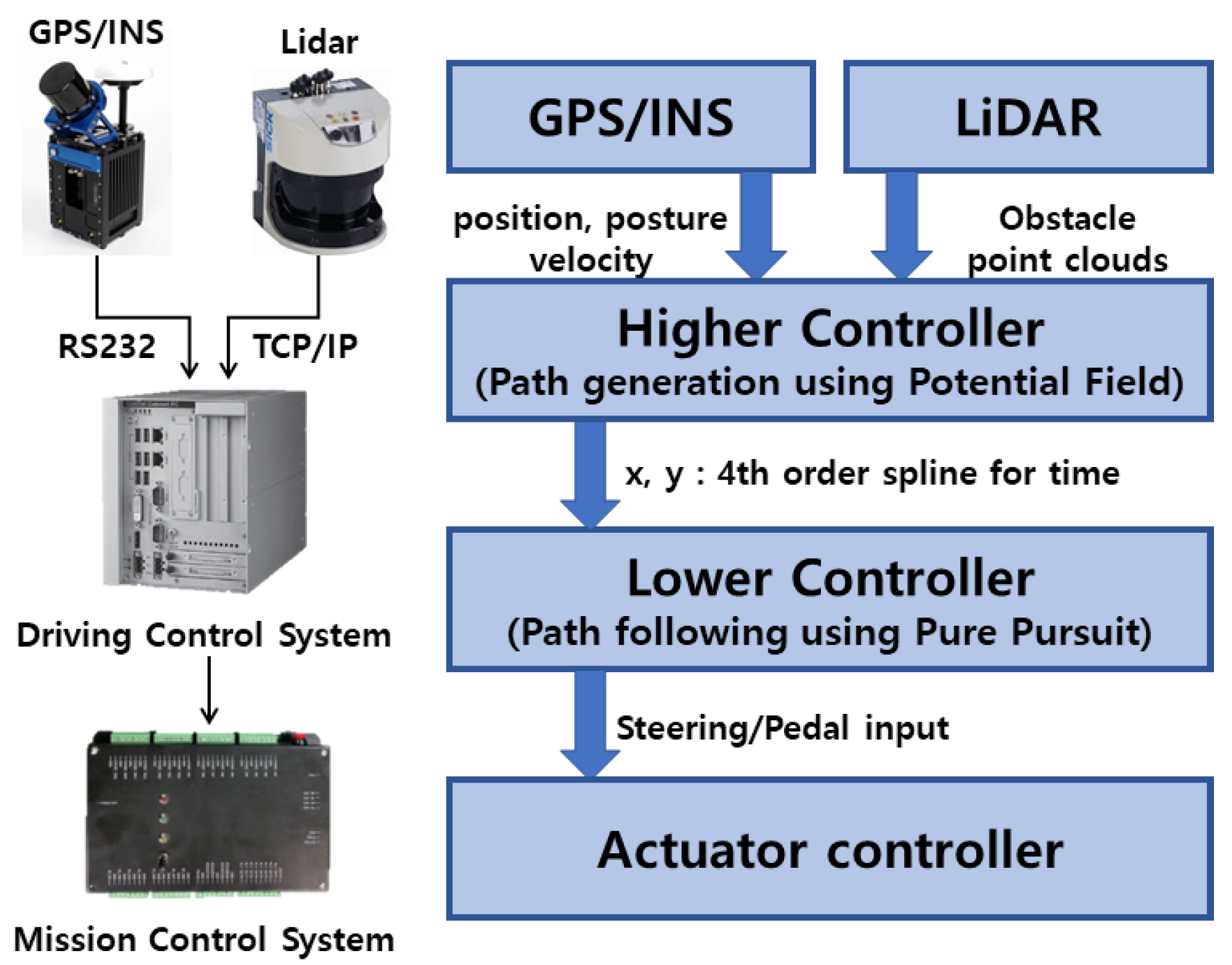
The autonomous driving algorithm is divided into upper control and lower control elements. In the upper control element, a path is generated by processing GPS/INS and LiDAR sensor signals, whereas, in the lower control element, steering control is performed to follow the created path. The potential field [21,22] algorithm was used for path generation, while the pure pursuit [23] algorithm was used for path tracking. A flow chart of the system is shown in Figure 3.

The location of obstacles is identified by fusion of distance information obtained from LiDAR and INS information. After creating a global path in a straight line from the current position to the waypoint with the waypoint received from the control system as the target point, a local path that can avoid obstacles is generated using the potential field algorithm.

$$U\left(q\right)=U_{att}\left(q\right)+U_{rep}\left(q\right).$$

(1)

$$U_{rep}=\{\begin{array}{cc}\min \left[\begin{array}{cc}{U}_{rep,max} ,& k{\left(\frac{1}{D}-\frac{1}{Q}\right)}^2\end{array}\right]& if D<Q\\ 0& else\end{array}$$

(2)

$$U_{att}=C\times l^2.$$

(3)

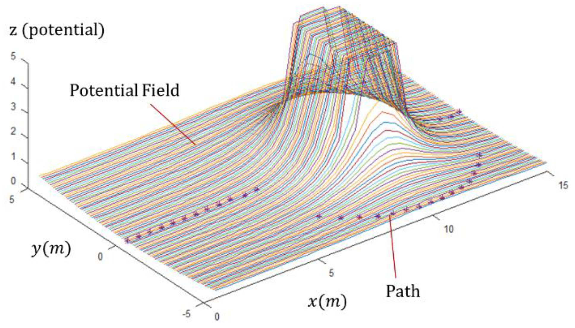
In Equation (1), q is a point in space, U_att is the attractive potential, U_rep is the repulsive potential, and U_rep,max is the maximum value of repulsive potential. D is the distance to the nearest obstacle, and k is the gain for calculating the repulsive potential. In order to consider only obstacles within the distance Q and to make the potential continuous, an equation is defined in the form of Equation (2). In Equation (3), C is the gain for calculating the attractive potential, and l is the perpendicular distance from q to the shortest path to the goal. When the global path is in the x-direction and there is an obstacle at (10, 0), the shape of the potential field is as shown in Figure 4.

A potential field is calculated at regular intervals in the direction perpendicular to the global path at regular intervals created using waypoints. At this time, U_att was defined to have a high potential in proportion to the square of the distance away from the path, and it moved along the point with the lowest potential.

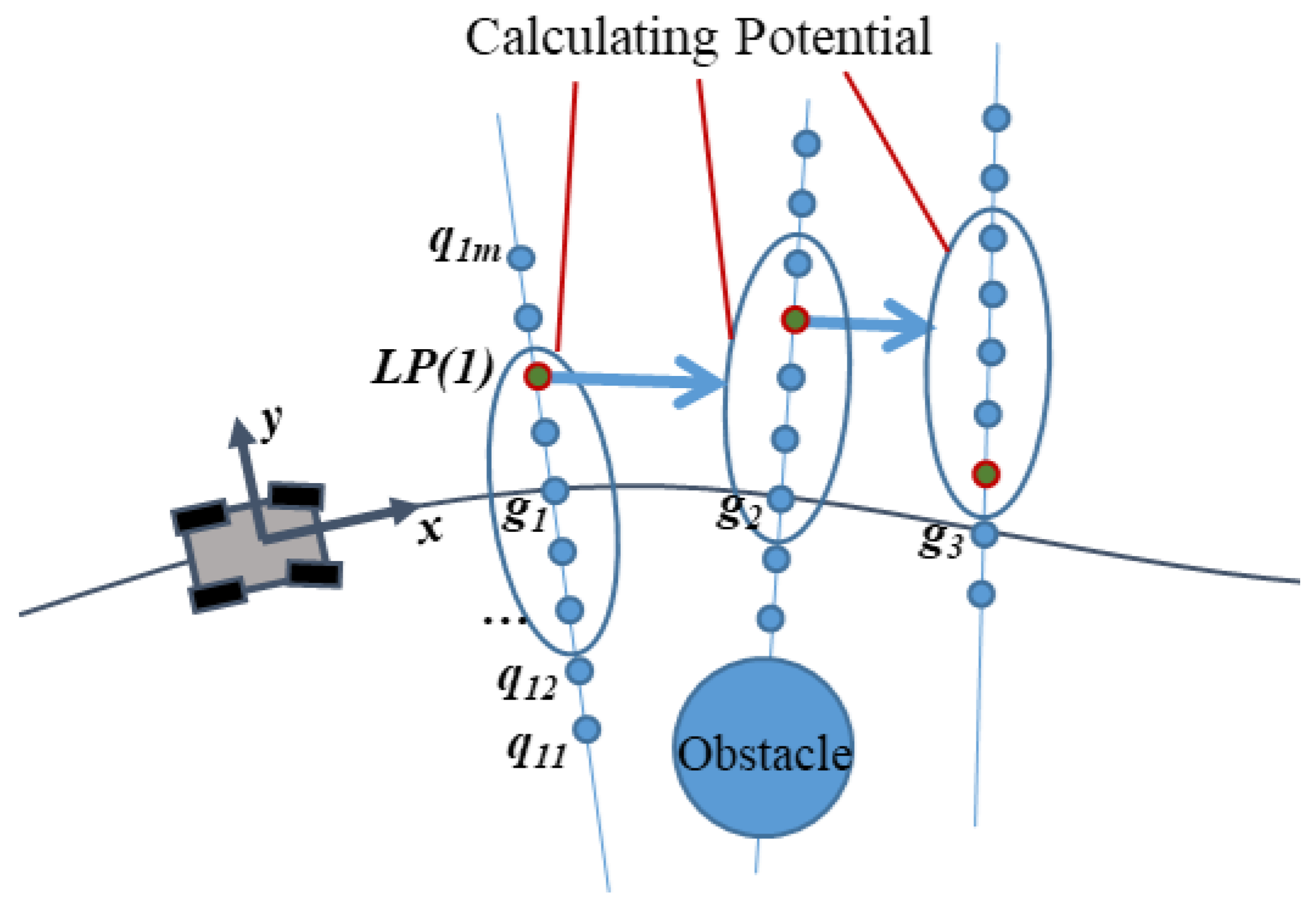
The potential field algorithm generally calculates the path after calculating the potential for all points in the domain. However, when the potential was calculated for all points in the domain in the DCS of the developed system, the operation time was intermittently exceeded. Since the developed electric vehicle featured rear-wheel driving and front-wheel steering, the area where the vehicle could reach the next time step was limited. Using this fact, instead of calculating the potential for all grids around the vehicle, the calculation was reduced by calculating only the potential in the reachable area, as shown in Figure 5 [25].

In the existing potential field, the global path is given as $G=\left\{g_1,g_2,\dots g_n\right\}$, and, in each $g_i$, there are $Q\left(g_i\right)=\left\{q_{i1},q_{i2},\dots q_{im}\right\}$ to calculate the $Potential\left(Q\left(g_i\right)\right).$ Furthermore, $\arg q_{min} Potential\left(Q\left(g_i\right)\right)$ is selected as the i-th local path LP(i). At this time, instead of calculating all of the $Potential\left(Q\left(g_i\right)\right)$ for $Q\left(g_i\right)$, the calculation time can be reduced by calculating the potential only for $Q\left(g_i\right)$ within a certain range from LP(i − 1). It is desirable to determine this range by considering the maximum steering angle of the vehicle and path_interval, which is the interval of the global path. In this paper, the ratio of the range and path_interval is expressed as potential_dist_ratio, and the simulations and experiments were performed for a value of 2.

3.2. Potential Field Algorithm Simulation

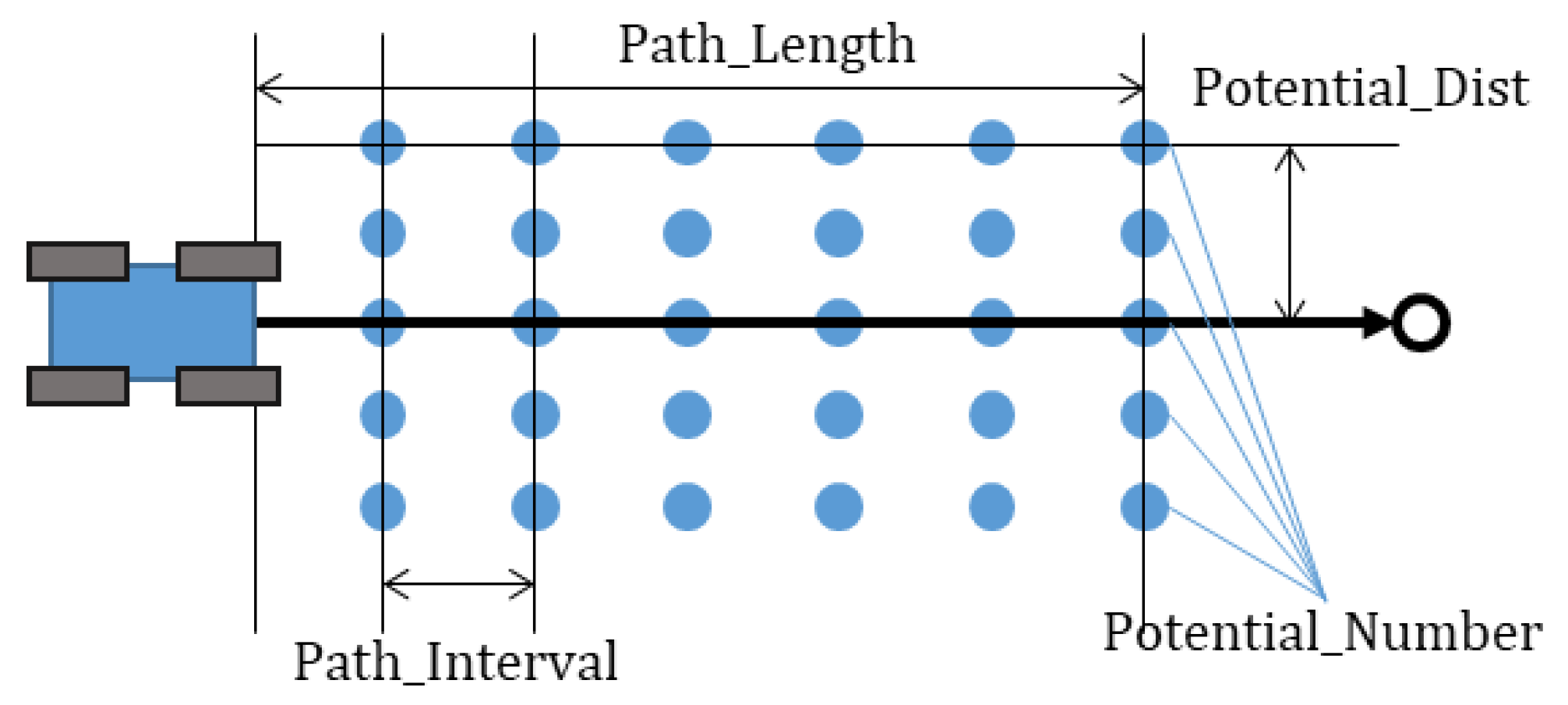
In order to perform autonomous driving by implementing the potential field algorithm, it is necessary to determine the importance of avoiding obstacles and maintaining the path by adjusting tunable variables. As shown in Figure 6, when the target and obstacles are positioned, the safe distance from the obstacle is determined by the variables k and C. And

Table 1. Simulation variables.

Variables
path_length	Length of local path generated by potential field algorithm
path_interval	Interval of global path (the shortest path)
K	Potential gain for obstacle
C	Potential gain for perpendicular distance from the global path
Q	Distance from obstacle to minimize potential
D_min	Distance from obstacle to maximize potential
Potential_Value_Max	Maximum potential value
potential_number	Number of potential calculation points
potential_dist	Perpendicular distance from global path to calculation potential
potential_dist_ratio	The ratio of distance in a normal direction to the driving direction to calculate potential

shows the description of each variable.

From Equations (1)–(3), the potential at each point is calculated as follows:

$$U\left(q\right)=k{\left(\frac{1}{D}-\frac{1}{Q}\right)}^2+C{l}^2.$$

(4)

If the constant C is defined as in Equation (5), a potential at a point L meters away from the global path has the same potential as a point with an obstacle within D_min. Therefore, the potential_dist and L must be determined in consideration of the size of the obstacles in the driving environment. If the created global path is blocked by an obstacle larger than L vertically from the global path, it is impossible to create a path that avoids the obstacle. In this study, L was set to about 5 m because there was no area blocked by a wall, and obstacles in the form of square pillars were used. The pseudo code of the Modified Potential Field algorithm is shown in Algorithm 1.

$$C=k{\left(\frac{1}{D_{min}}-\frac{1}{Q}\right)}^2\frac{1}{L^2}.$$

(5)

Algorithm 1: Pseudo code of modified potential field algorithm

1: Creates a global path at regular intervals(path_interval) as long as path_length 2: //initialize variables: local path, index_min 3: local path = current position 4: index_min = potential_number × 0.5//index of current position 5: fori = 1: number of global path points 6:   //Select points to calculate potential in the direction perpendicular to the global path 7:   for index = 0: potential_number 8:     q(index) = global path(i) + perpendicular vector × (index − potential_number × 0.5) 9:   end for 10:   //N: number of points to calculate potential 11:   N = potential_dist/potential_number × potential_dist_ratio 12:   for j = index_min − N:index_min + N 13:     //find the nearest obstacle point cloud from q(j) 14:     D = min($\mathrm{point}\mathrm{cloud}-q\left(j\right)$) 15:     $l$ = perpendicular vector × (index − potential_number × 0.5) 16:     //calculate potential of q(j) 17:     potential = ${\left(\frac{1}{D}-\frac{1}{Q}\right)}^2+C{l}^2$ 18:     //find q with minimum potential 19:     if potential < potential_min 20:       potential_min = potential 21:       index_min = index 22:     end if 23:   end for 24:   local path = local path + q(index_min) 25: end for

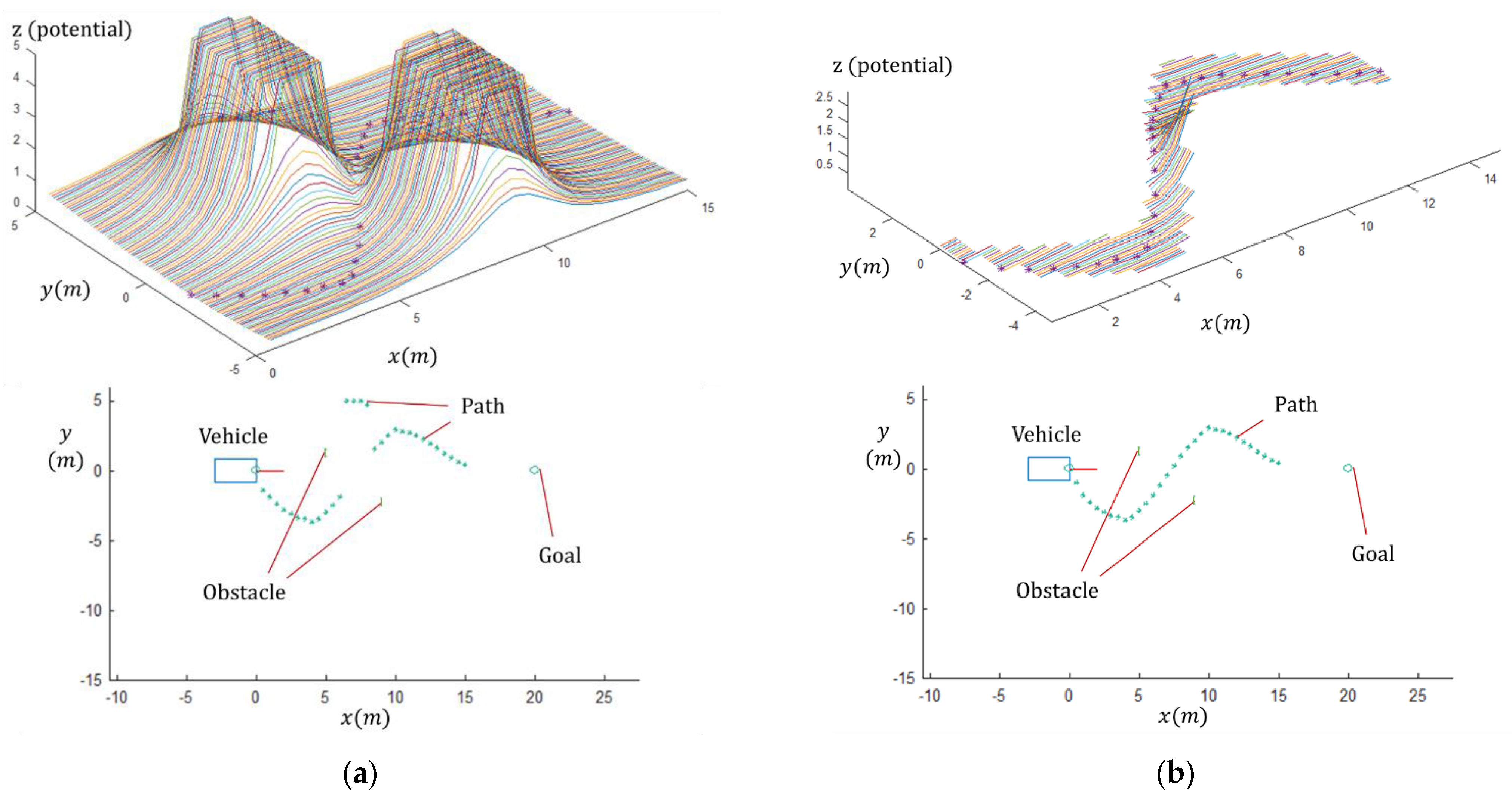
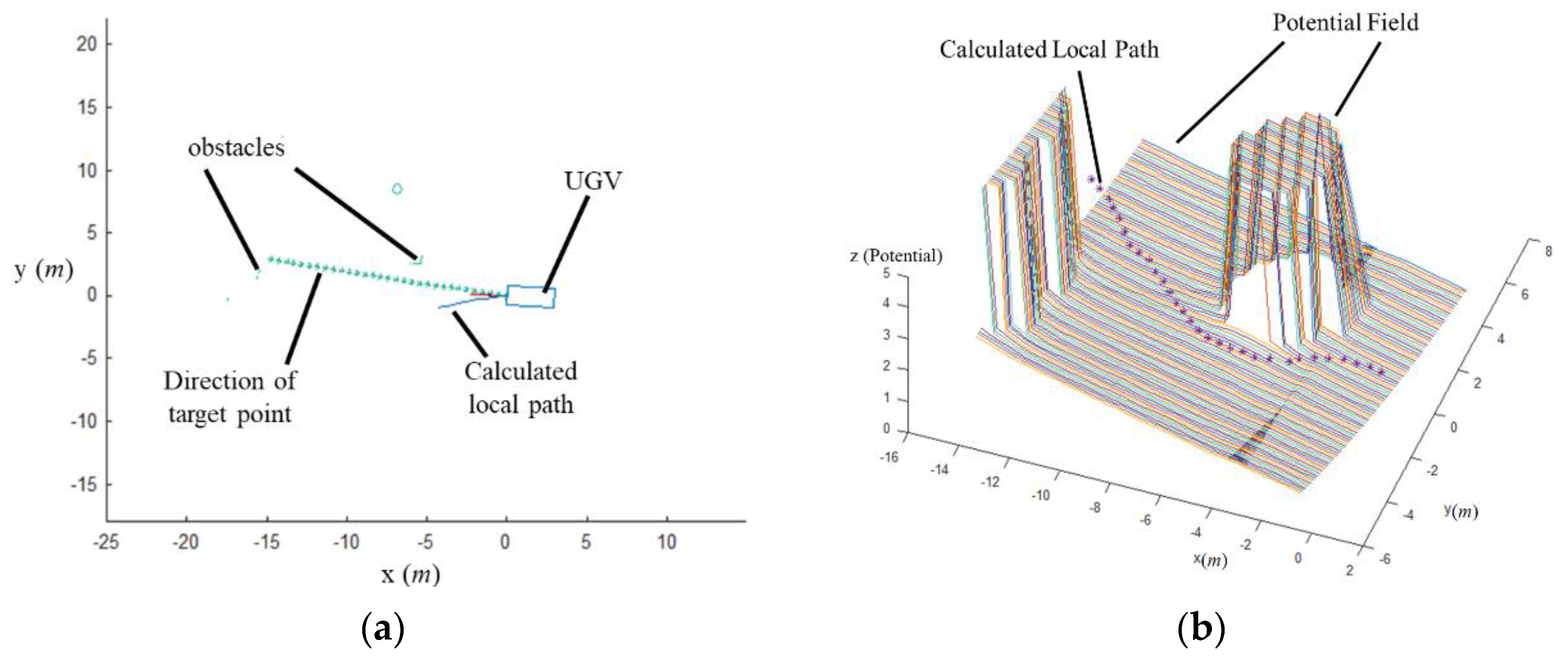
When L is 5 m, the starting point is (0, 0), the target position is (20, 0), and the obstacle position is (10, 0), the potential field and path shown in the Figure 7 are created. The vehicle changes direction about 4 m in front of the obstacle and drives 3.8 m away from the obstacle. Figure 7a is the result of calculating the potential field for all points, while the result of applying the modified method is shown in Figure 7b. In the modified method, the potential is calculated only for some regions, and the generated path is the same as for the existing method.

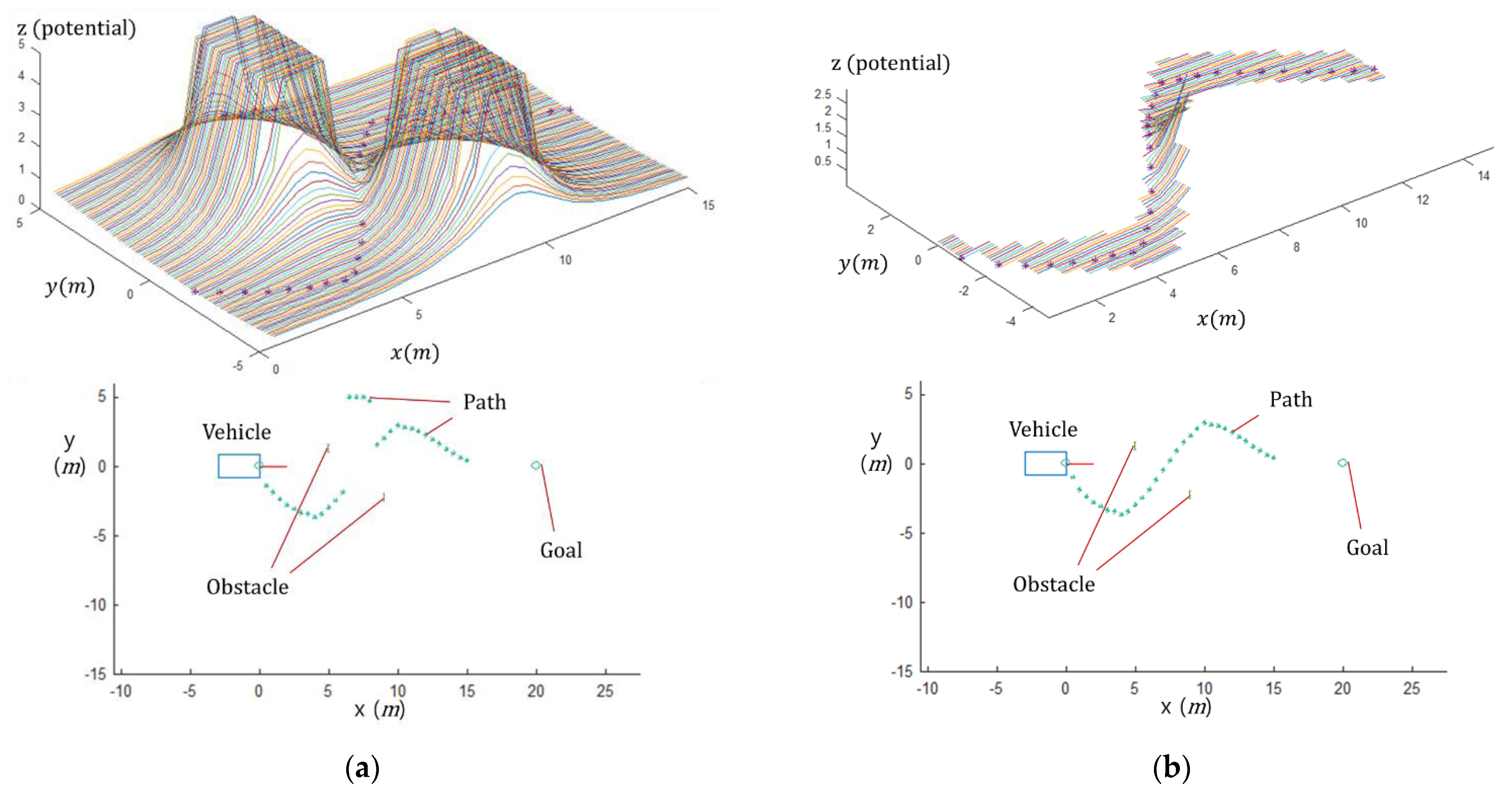
As shown in Figure 8a, in the situation of passing between two obstacles, when the potentials are calculated for all points and the points having the minimum value are selected, the path is cut off because the point that cannot be reached has the minimum potential. On the other hand, in Figure 8b, a smooth path was created because the potential was calculated only for a certain region in the next timestep on the basis of the point with the minimum potential.

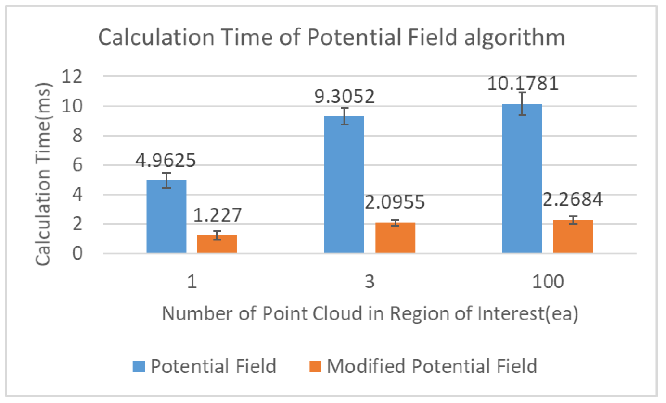
In the modified potential field algorithm, the amount of computation is reduced because the potential is calculated only for some areas. Since both methods calculate the potential using the distance to the nearest obstacle among the point clouds in the region of interest, the calculation time varies according to the number of point clouds. In order to compare the computation time of the potential field and the modified potential field when the number of point clouds is one, three, or 100, the average computation time and standard deviation were obtained by performing 1000 calculations under the conditions shown in

Table 2. Simulation environment.

CPU	Intel® Core™ i7-8559U 2.70 GHz
RAM	16 GB
OS	Windows 10 64 bit
Path_length	15 m
Path_interval	0.5 m
k	10
L	10 m
Q	10 m
D_min	1.5 m
Potential_Value_Max	5
Potential_number	100
Potential_dist	5 m
potential_dist_ratio	2

; the results are shown in Figure 9.

Since the LiDAR mounted on the UGV updates the new point cloud at a frequency of 10 Hz, the path generation frequency was also set to 10 Hz. The existing method took about 10% of the time to create a path at each step, whereas the modified method showed an improvement to 2% of the time.

4. Driving Test

4.1. Multiple Obstacle Avoidance Experiment

Assuming that a single operator operates several unmanned vehicles, there are many difficulties in providing the UGV with a route point to avoid obstacles. Therefore, when one target point is given and obstacles exist between the target points, the aim was to show whether the UGV could avoid the obstacle by itself.

In order to realize such a situation, the obstacles were arranged such that the four obstacles had to be avoided alternately left and right. As shown in Figure 10, the distance between obstacles was approximately 15 to 20 m in the driving direction, and about 3 to 5 m in the perpendicular direction.

Figure 11 shows the UGV moving while avoiding obstacles, while Figure 12a shows the UGV trajectory and surrounding obstacles as a graph. The speed and the steering graph of the UGV are shown in Figure 12b. Steering was expressed as a percentage for a maximum of 0.5 rad, while speed was expressed by multiplying by 10 for visualization in m/s.

Figure 13 shows the situation of the UGV and surrounding obstacles at a specific timepoint during obstacle avoidance. The UGV moved toward the target point in the west direction, before steering to the left to avoid the first obstacle, at which point the second obstacle appeared. Since it is inefficient to store all potentials in real time, we saved the position log of the UGV and obstacles and reconstructed the potentials after the experiment. The values of the parameters applied to the experiment are shown in

Table 3. Driving test environment.

Path_length	15 m
Path_interval	0.5 m
k	10
L	10 m
Q	10 m
D_min	1.5 m
Potential_Value_Max	5
Potential_number	100
Potential_dist	5 m

.

4.2. Multiple UGV/UAV Operation Test

In order to operate two or more UGVs at the same time, autonomy must be secured. Since the operator has to simultaneously control several unmanned vehicles, it is impossible to always give a new waypoint to the UGV. Therefore, the operator gave the area to the UGV and implemented the function to repeatedly search the given area for the UGV to conduct the experiment [25].

According to a predefined air pollution mapping scenario [26], shown in Figure 14, one person simultaneously controlled two UGVs and three UAVs, and several unmanned vehicles searched a space at the same time. Figure 15 shows the two UGVs and three UAVs operating at the same time, while Figure 16 shows the GPS log and obstacle point cloud graphs of the two UGVs and the speed and steering graphs of each UGV. When a region was given to the UGV, vertices were selected as waypoints and followed sequentially and repeatedly in a clockwise direction. If there was an obstacle, it was avoided according to the driving algorithm. In the simulation of Figure 7, it can be seen that a path avoiding the obstacle was created about 5 m in front of the obstacle. In the GPS log of UGV #1 in Figure 16a, it can be confirmed that the vehicle changed direction about 5 m in front of the obstacle. Furthermore, since the UGV was traveling clockwise, it continued to steer in one direction. As shown in the graph of Figure 16b, it steered in the negative direction after steering in the positive direction to avoid an obstacle. Images of the UGV avoiding obstacles are shown in Figure 17.

5. Discussion

In this study, the system configuration of a UGV used for ground–aerial cooperation was briefly introduced, and an efficient path-planning method for autonomous driving of the UGV in real time was introduced. For real-time path planning, not only the stable avoidance of obstacles but also the calculation speed is very important. Although a simple and efficient potential field algorithm was selected, the computation time was insufficient. To overcome this, a method to reduce the amount of computation by using the vehicle’s steering characteristics was proposed.

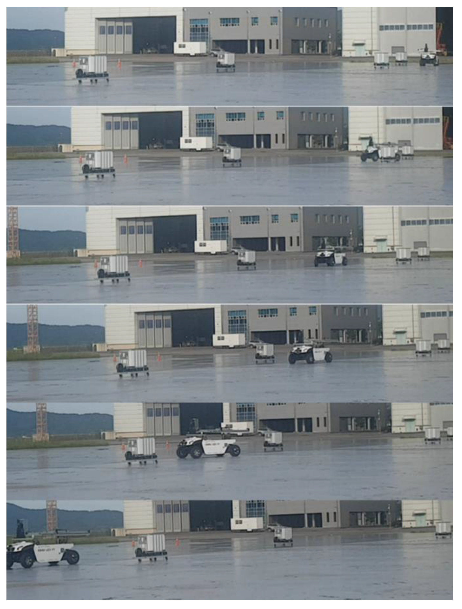
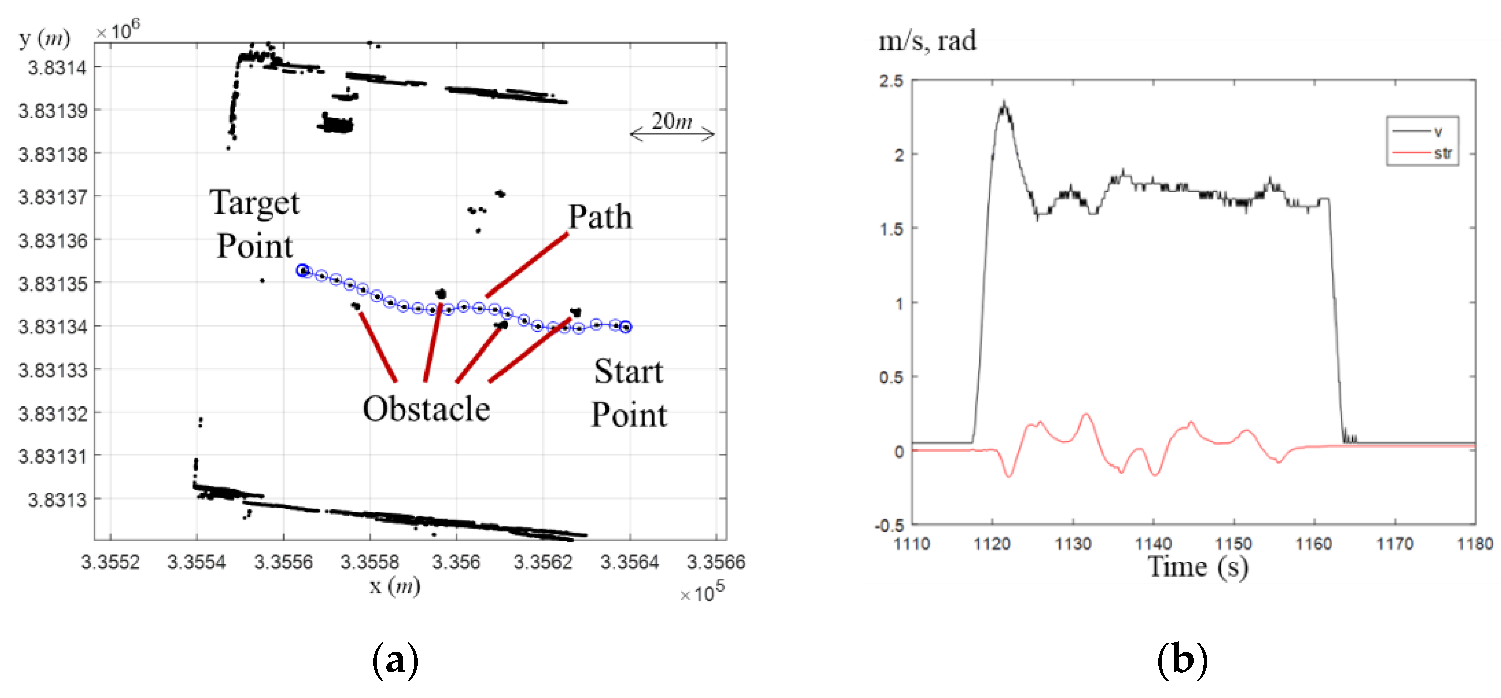
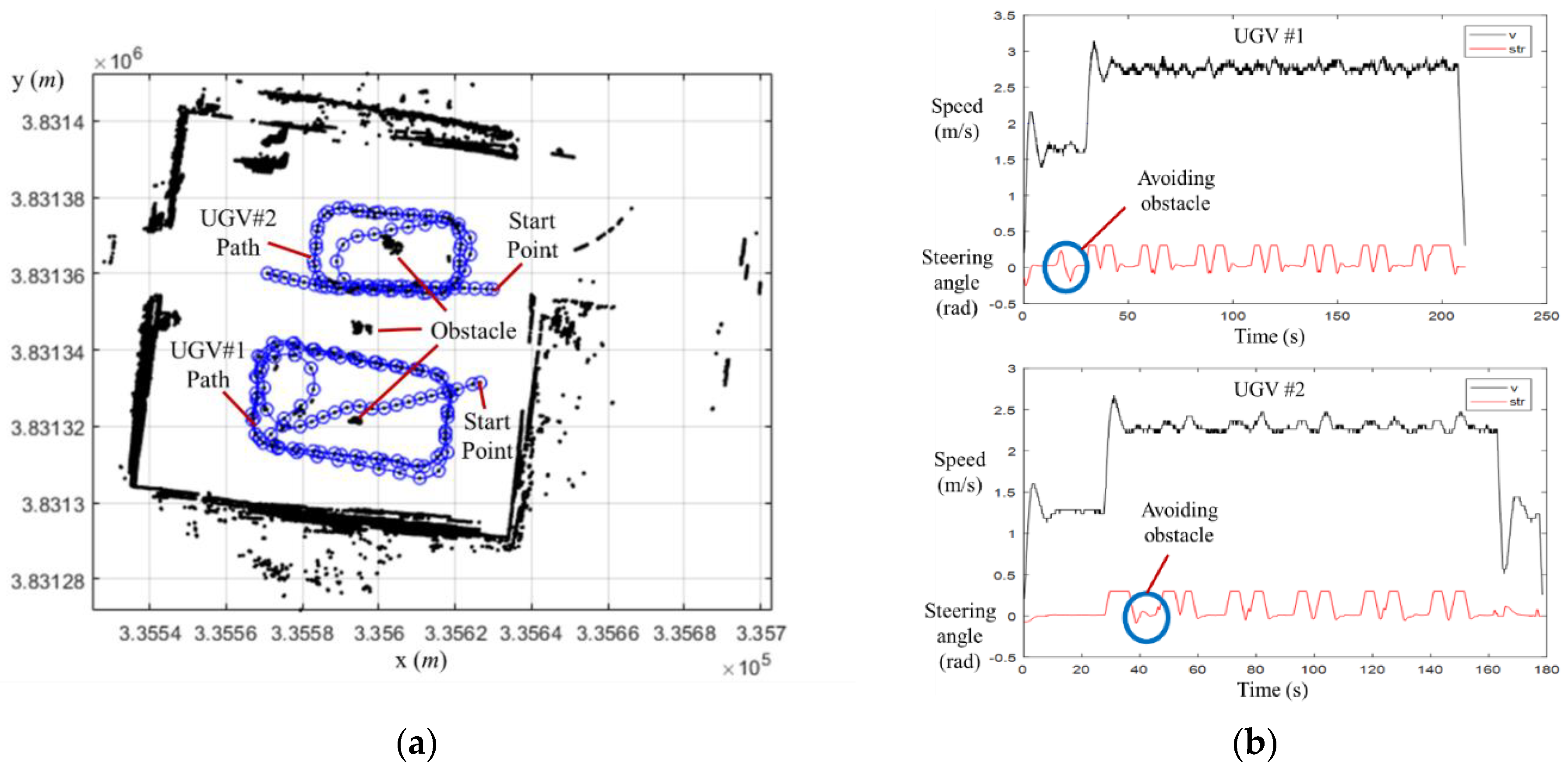
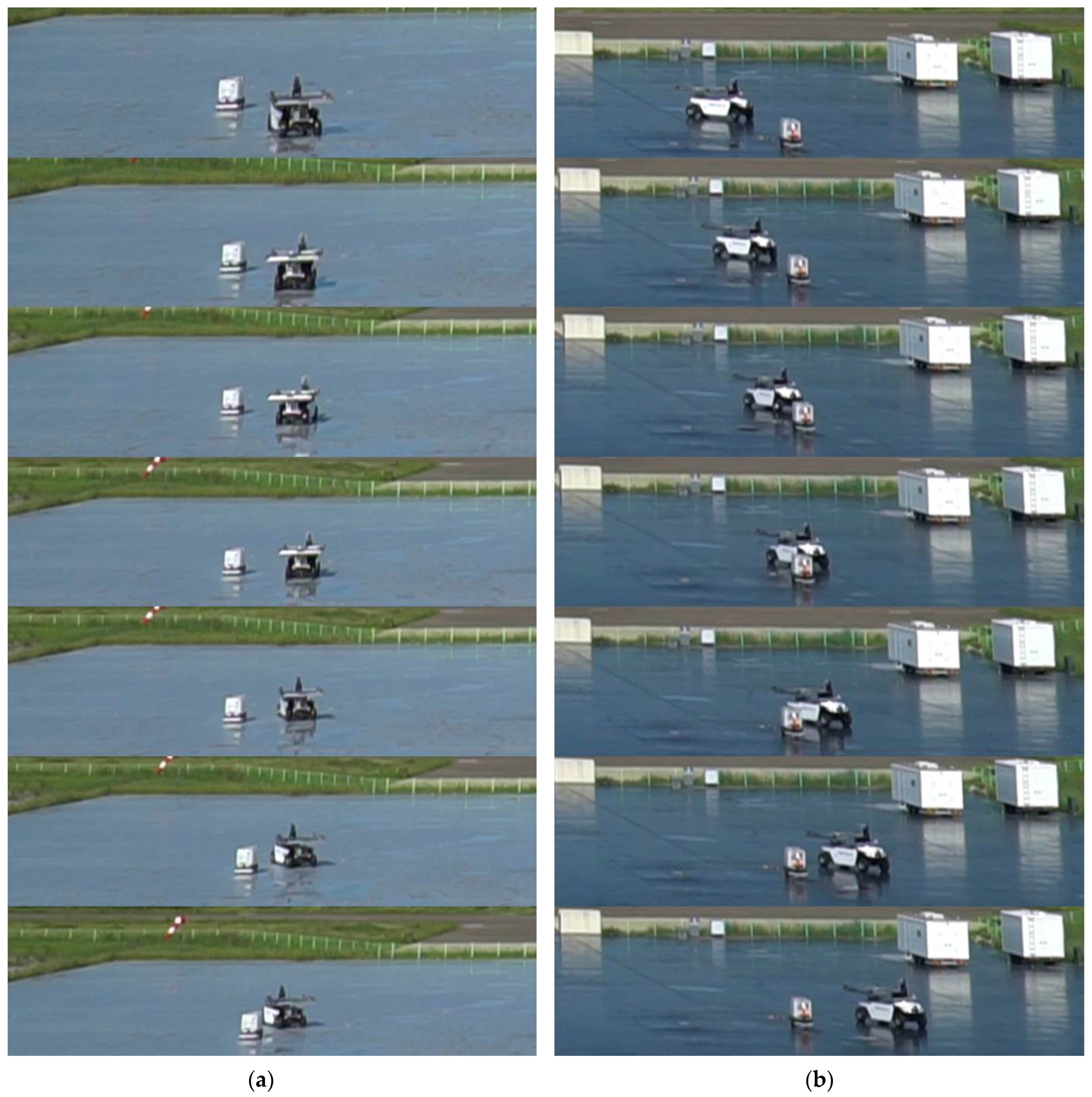
Through the simulation, it was shown that the results of path generation and the existing method were not significantly different, and the calculation time was reduced compared to the existing method by measuring the calculation time. Then, a driving experiment was performed by applying the algorithm to the UGV, and it was confirmed that the UGV avoids obstacles in the driving path.

Despite the existence of various path-planning algorithms, path-planning methods are still needed to be used in a situation in which the controller needs to perform various tasks, including path planning, or a controller is needed with low computational performance. The method proposed in this paper is expected to be particularly suitable for controlling a vehicle equipped with a low-spec controller.