
Data Extraction Method for Industrial Data Matrix Codes Based on Local Adjacent Modules Structure

Abstract
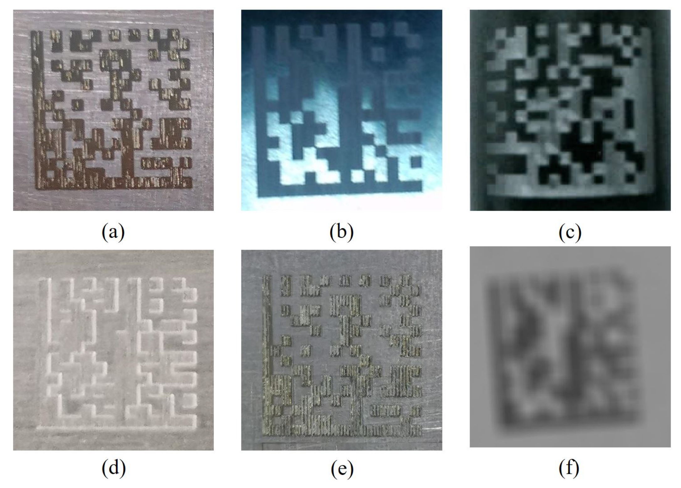
:1. Introduction
2. Related Works
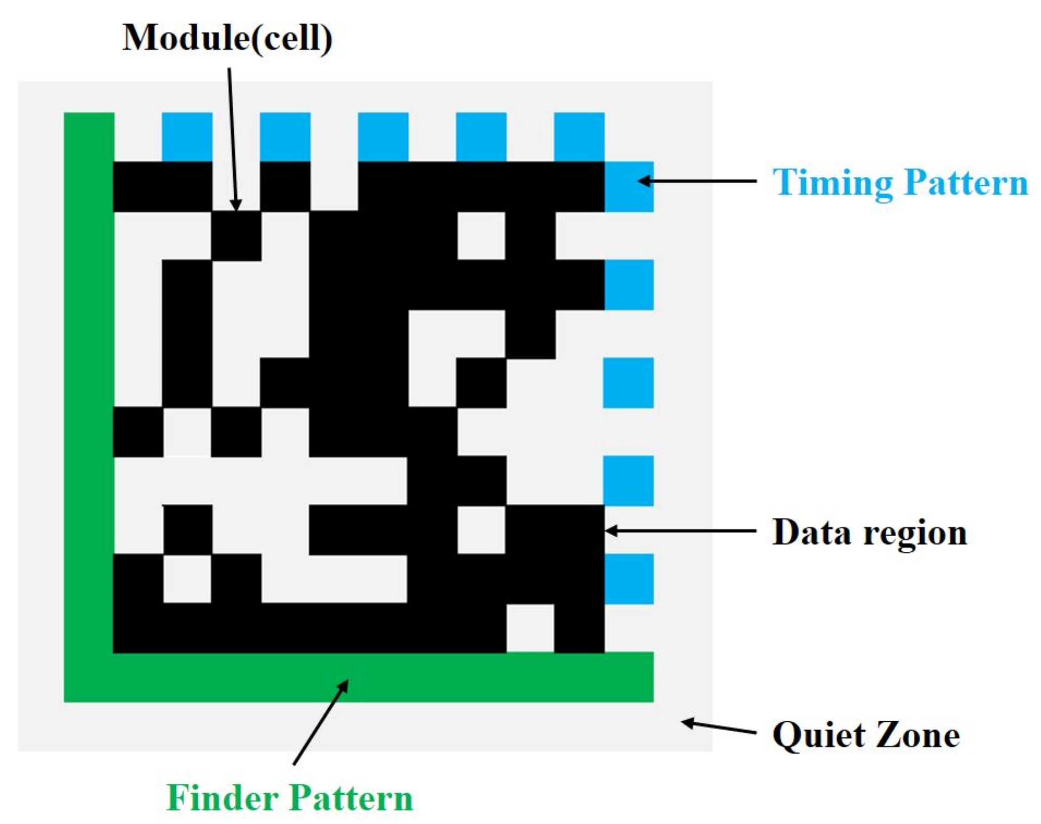
3. The Graph Structure of the DM Symbol
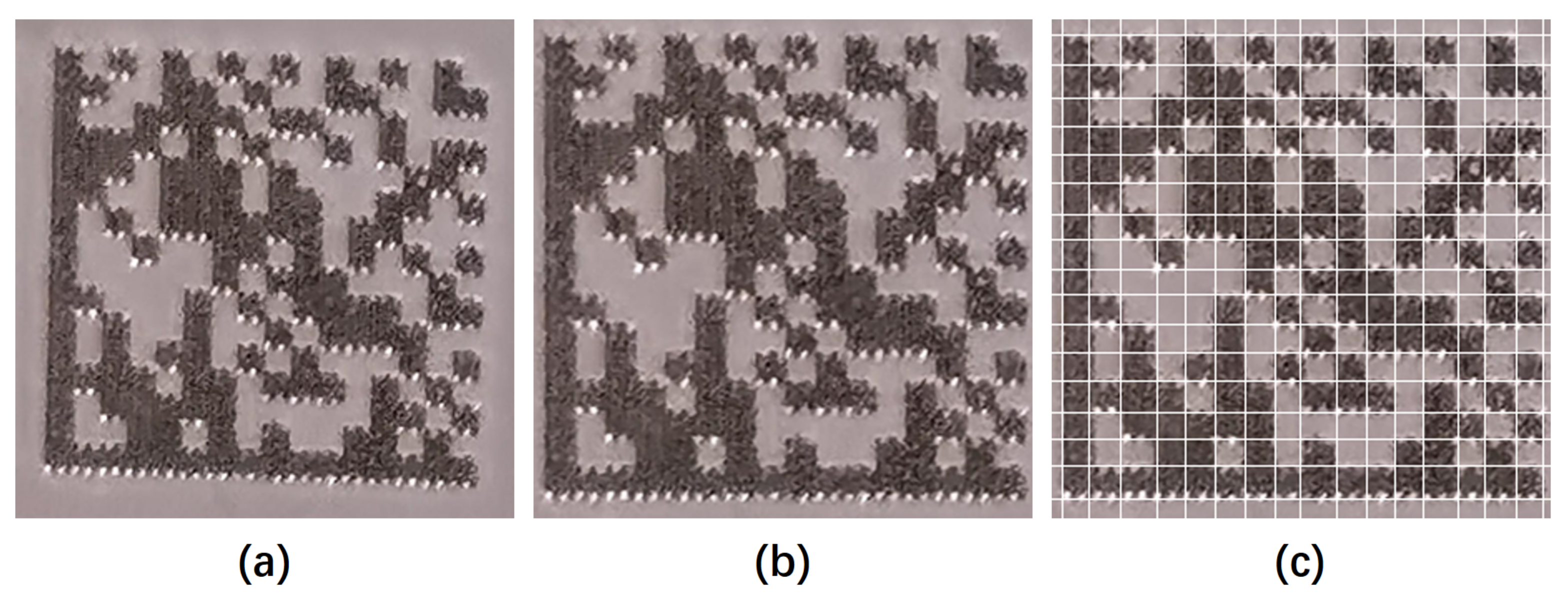
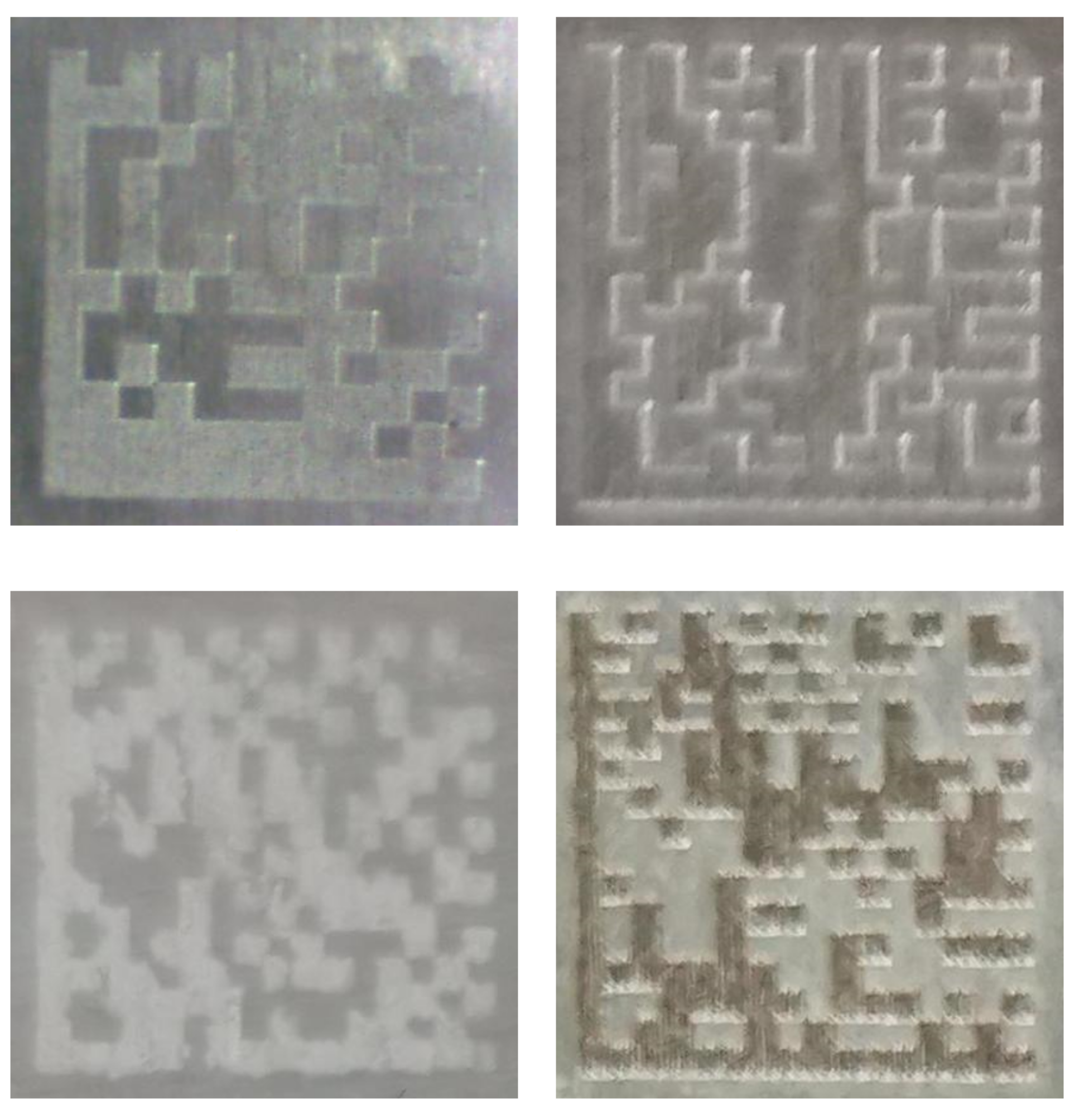
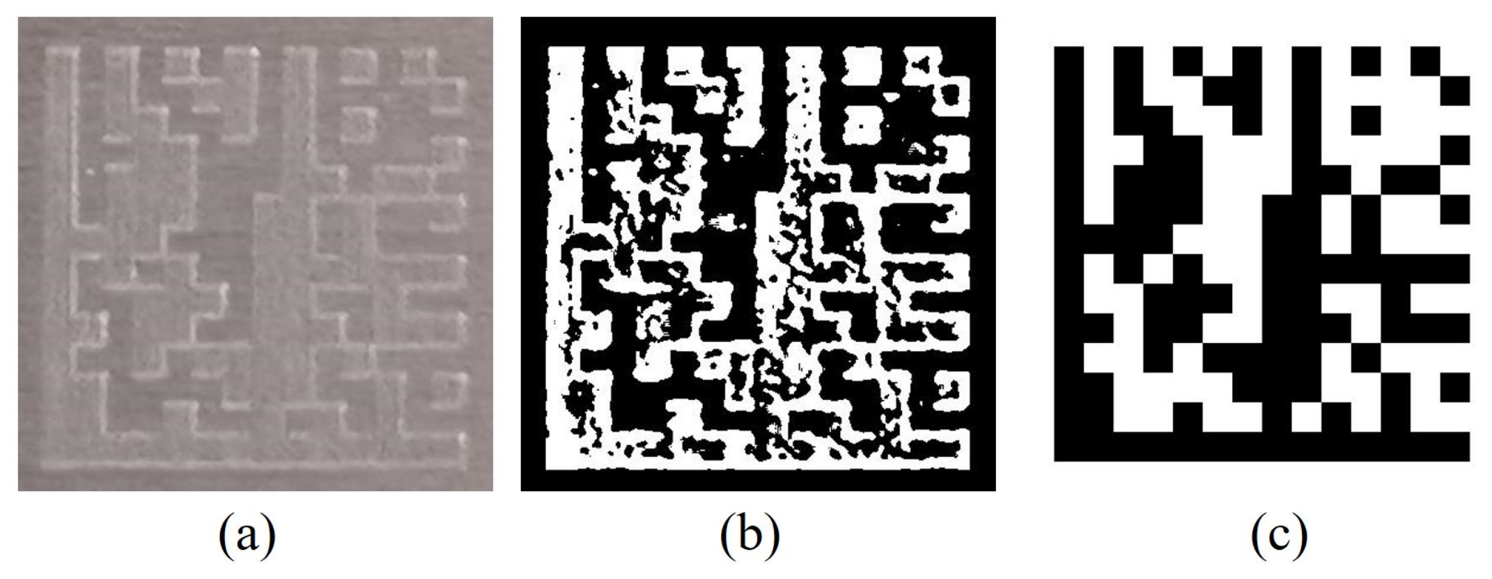
4. Barcode Image Pre-Processing
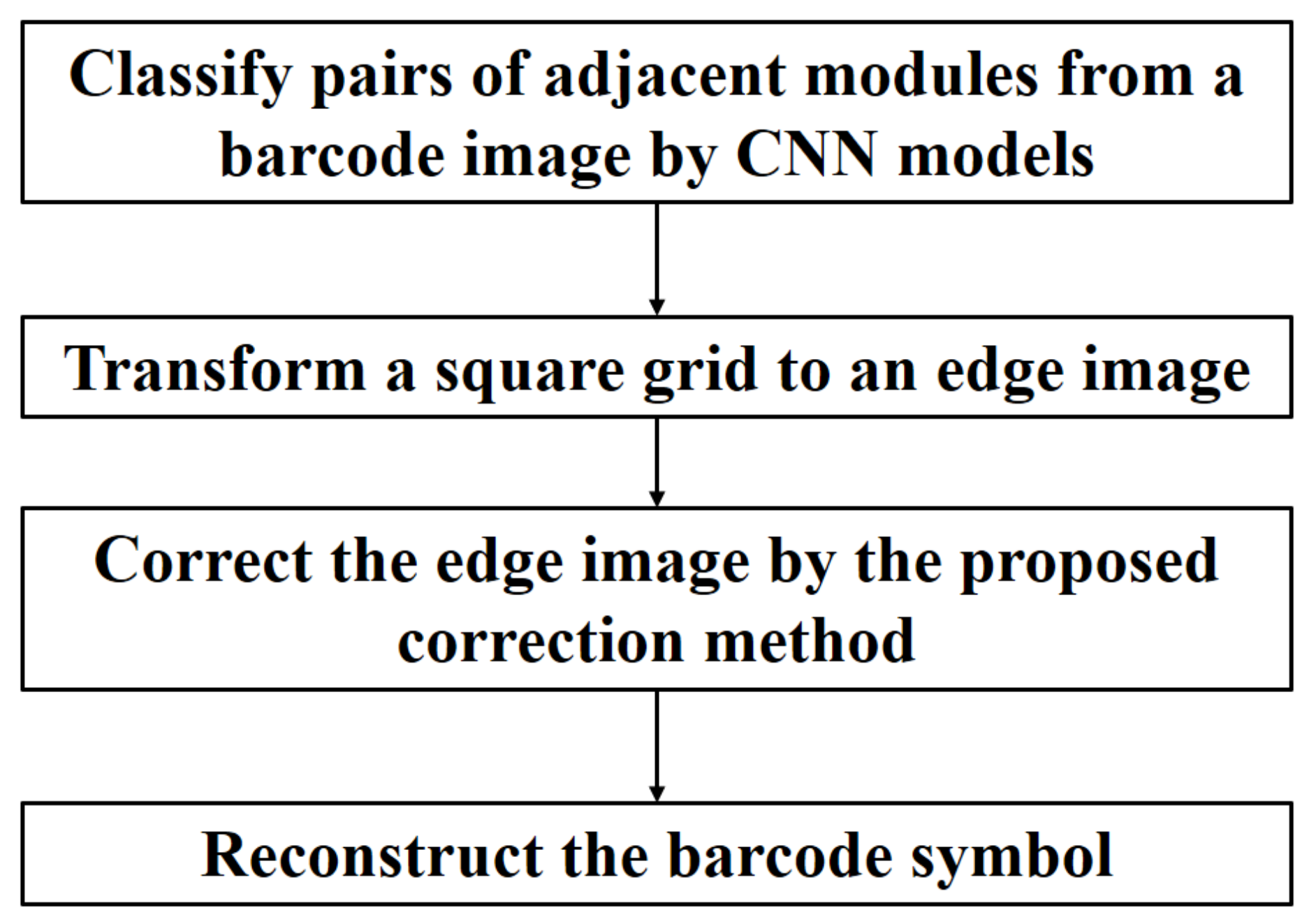
5. Barcode Data Extraction
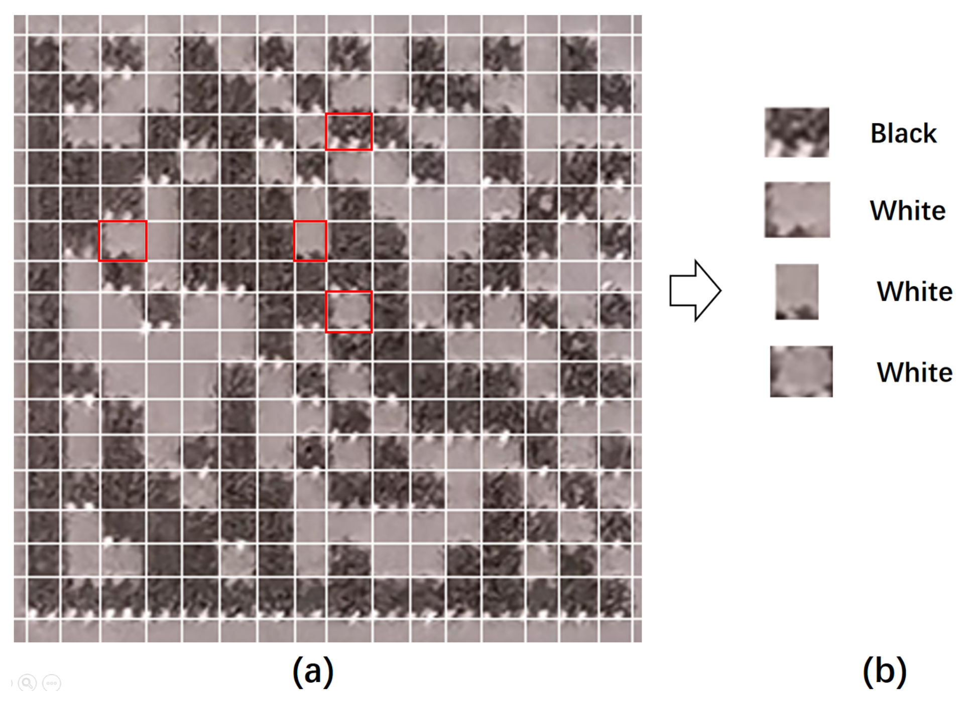
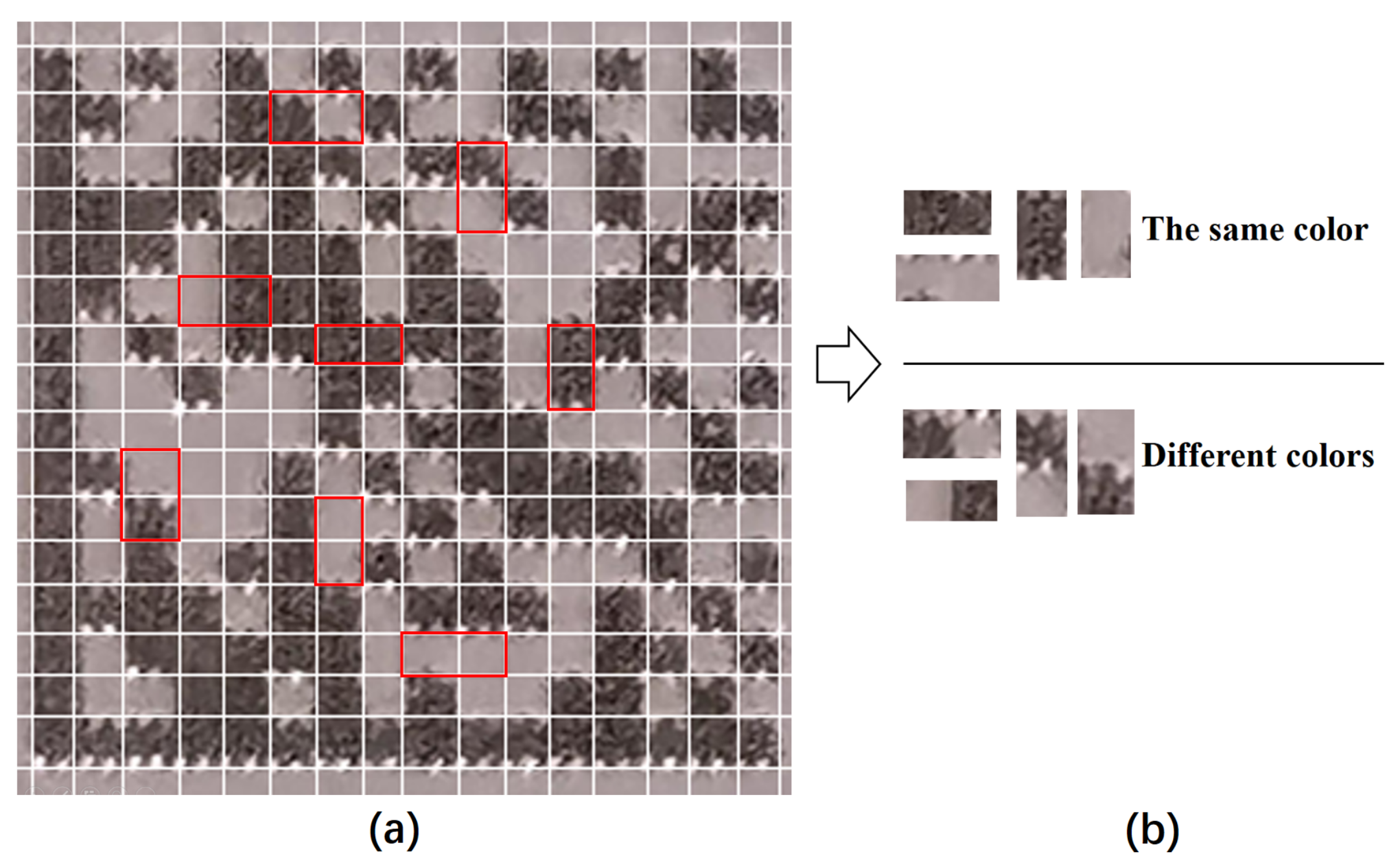
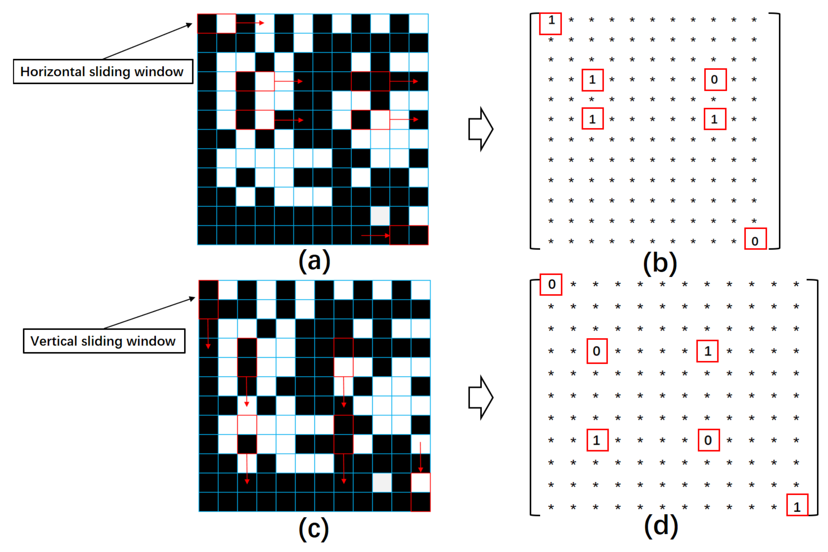
5.1. Classify Pairs of Adjacent Modules by CNN
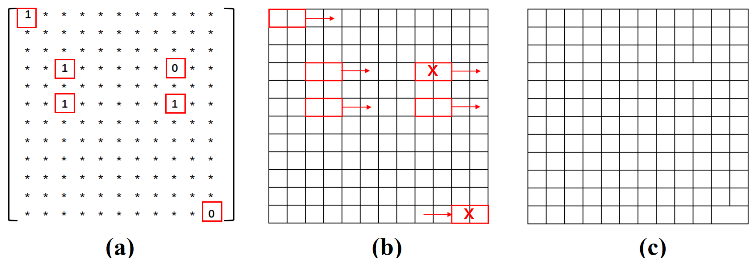
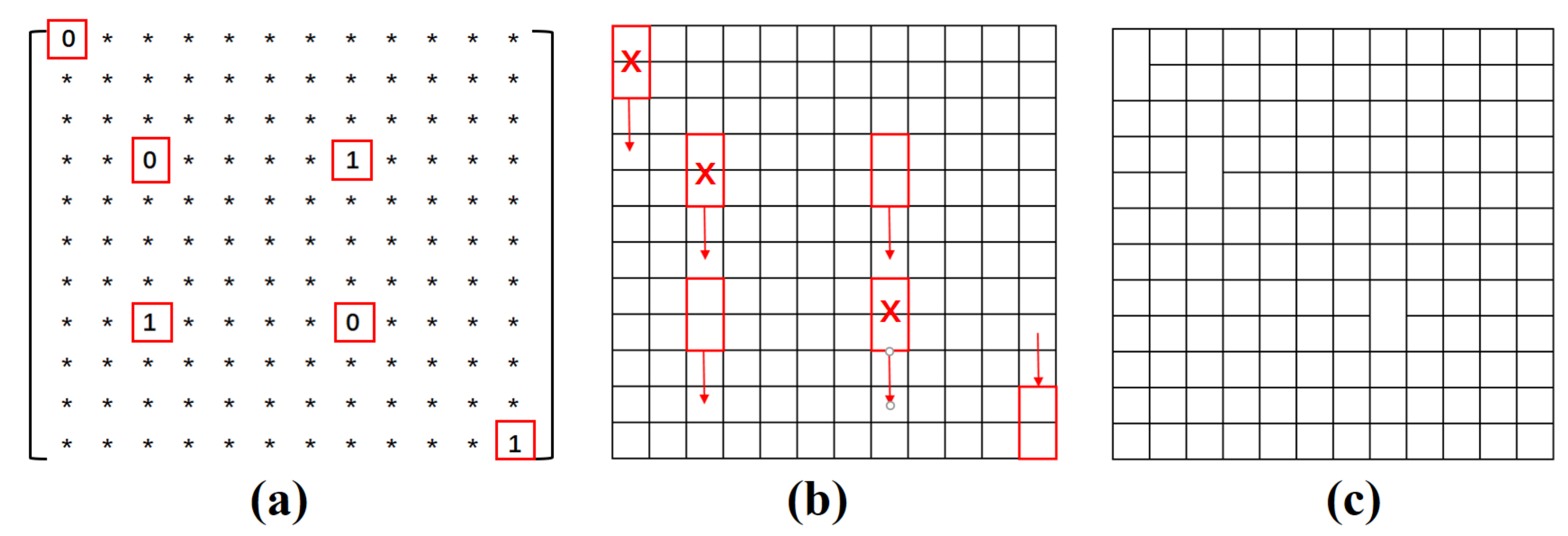
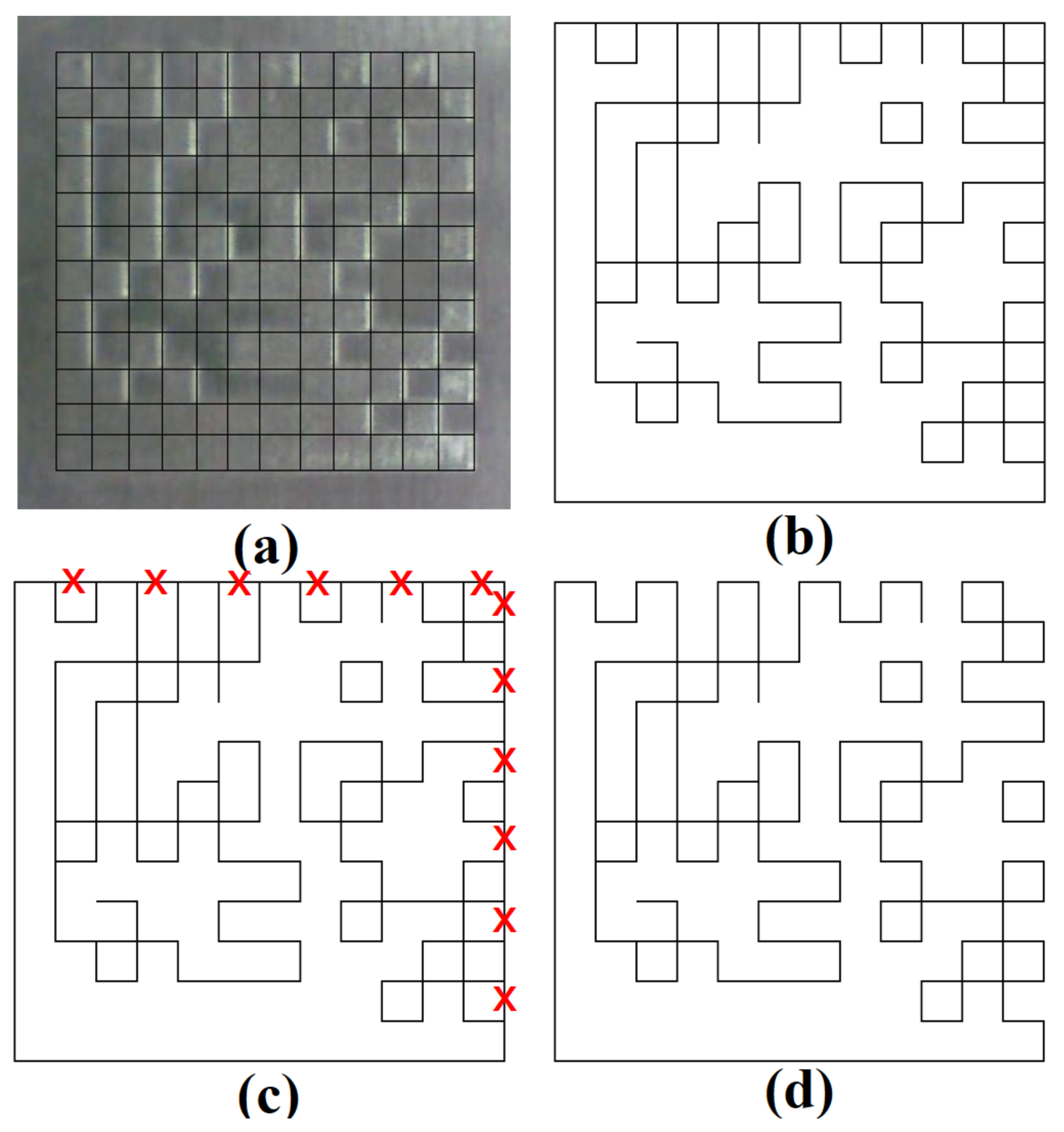
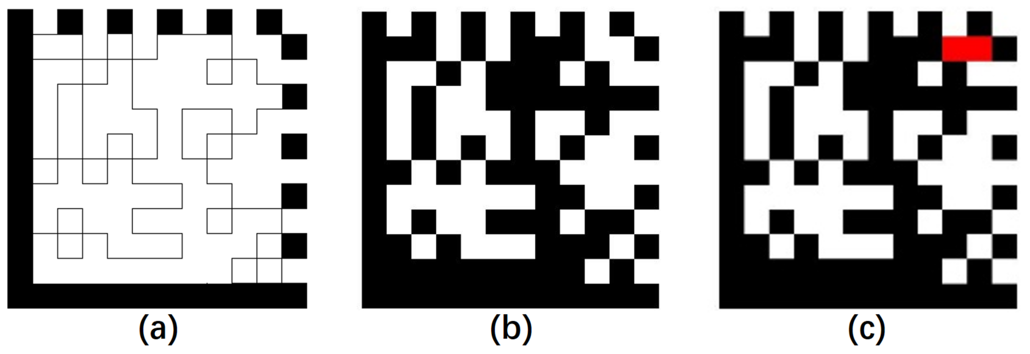
5.2. Transform a Square Grid Format Image to an Edge Image
5.3. Transform a Square Grid Format Image to an Edge Image
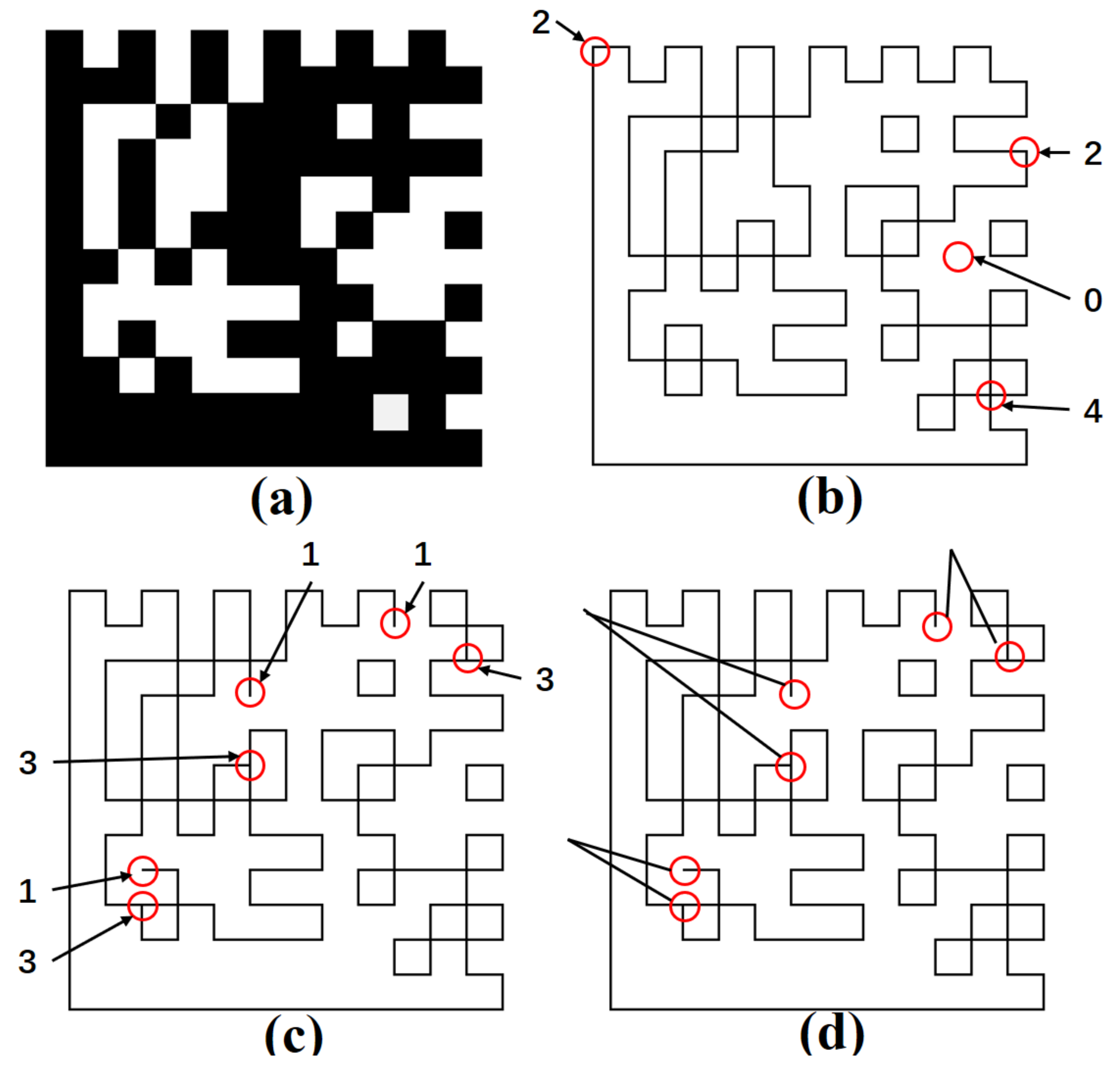
5.3.1. Pair Odd-Degree Vertices in the Edge Image
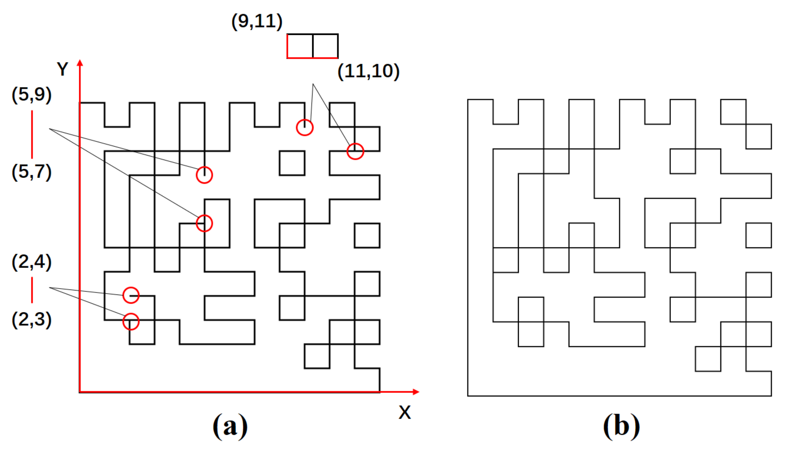
5.3.2. Correct the Edge Image by Eliminating Pairs of Odd-Degree Vertices
5.4. Barcode Reconstruction and Recognition
6. Experiment Results
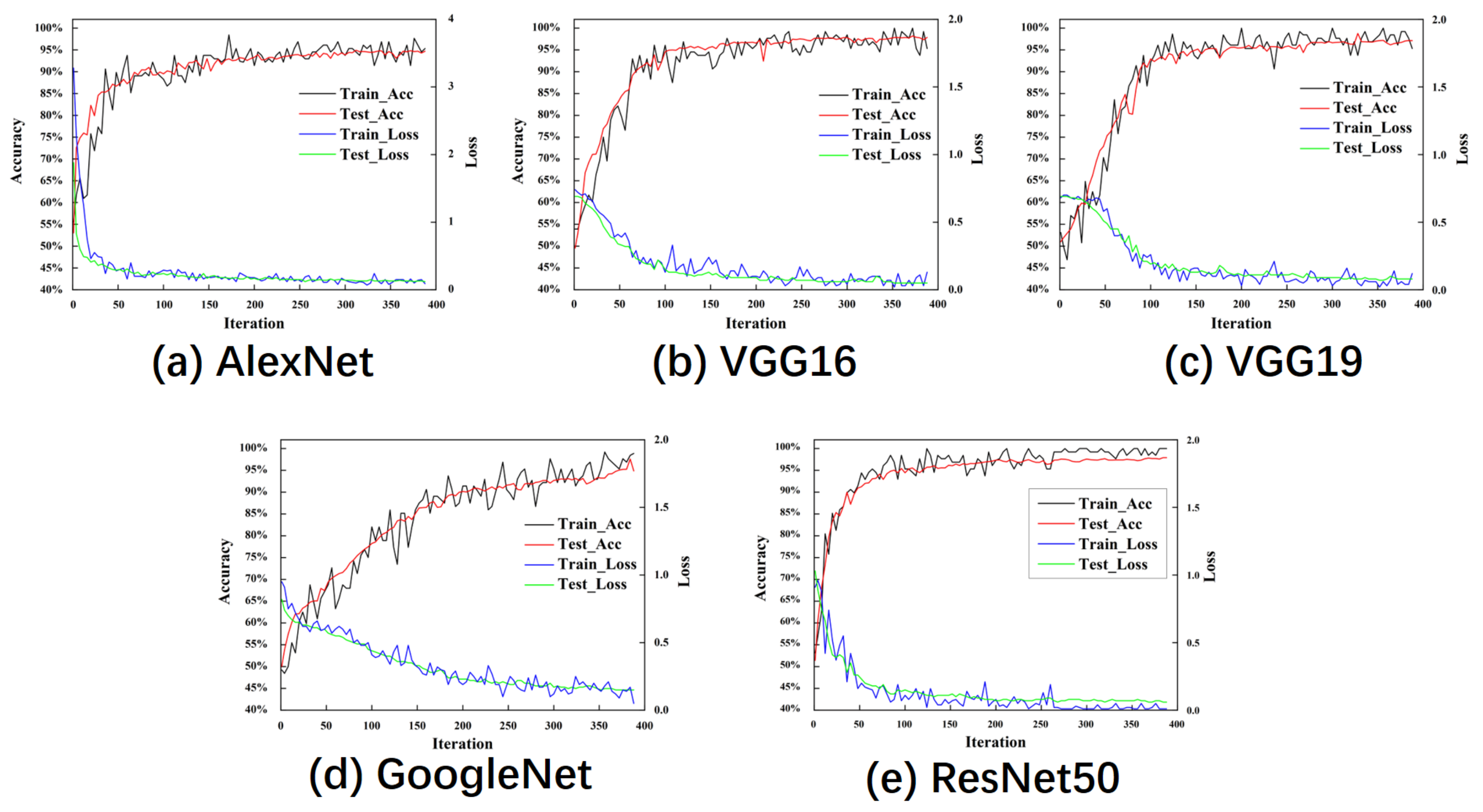
6.1. Training and Verification of CNN
6.2. Test Results of CNN
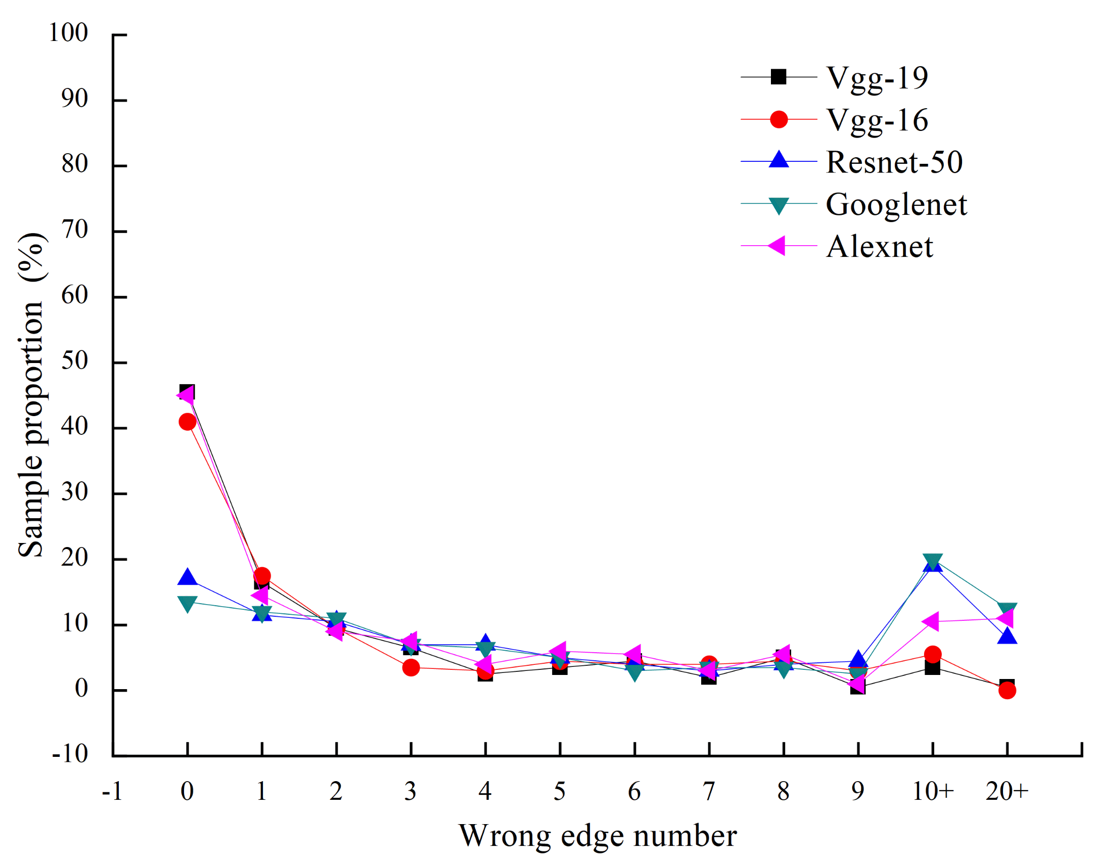
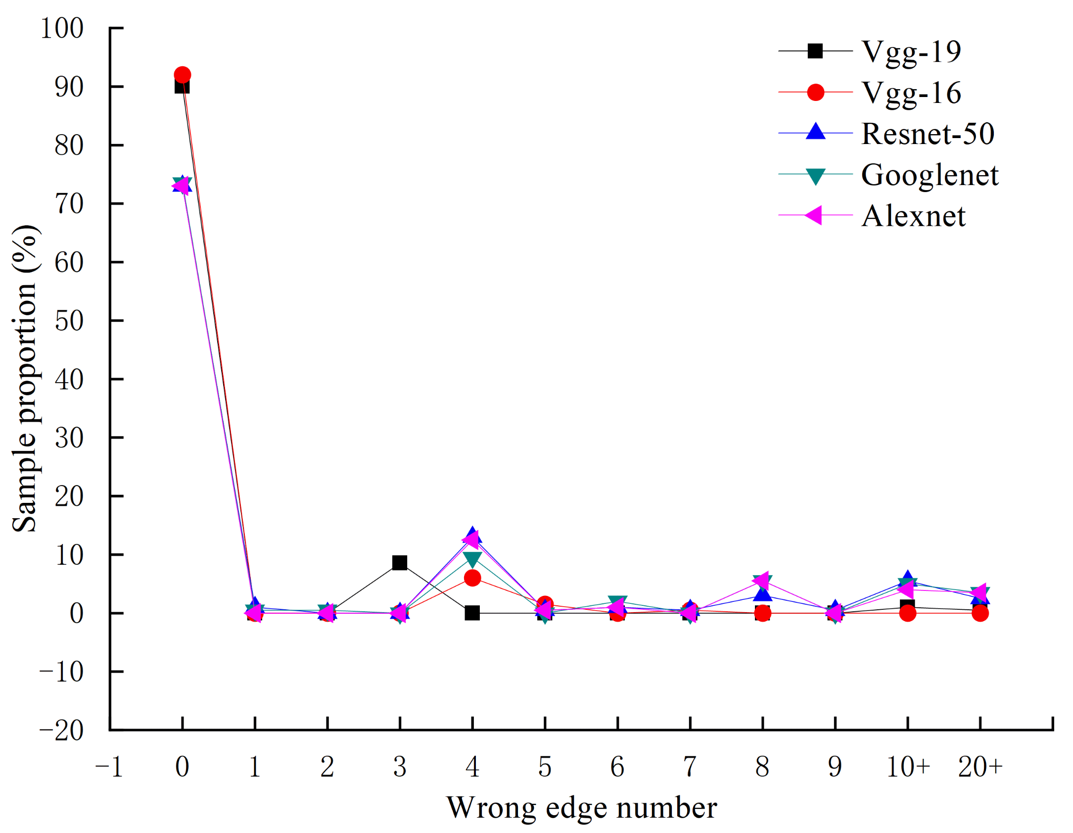
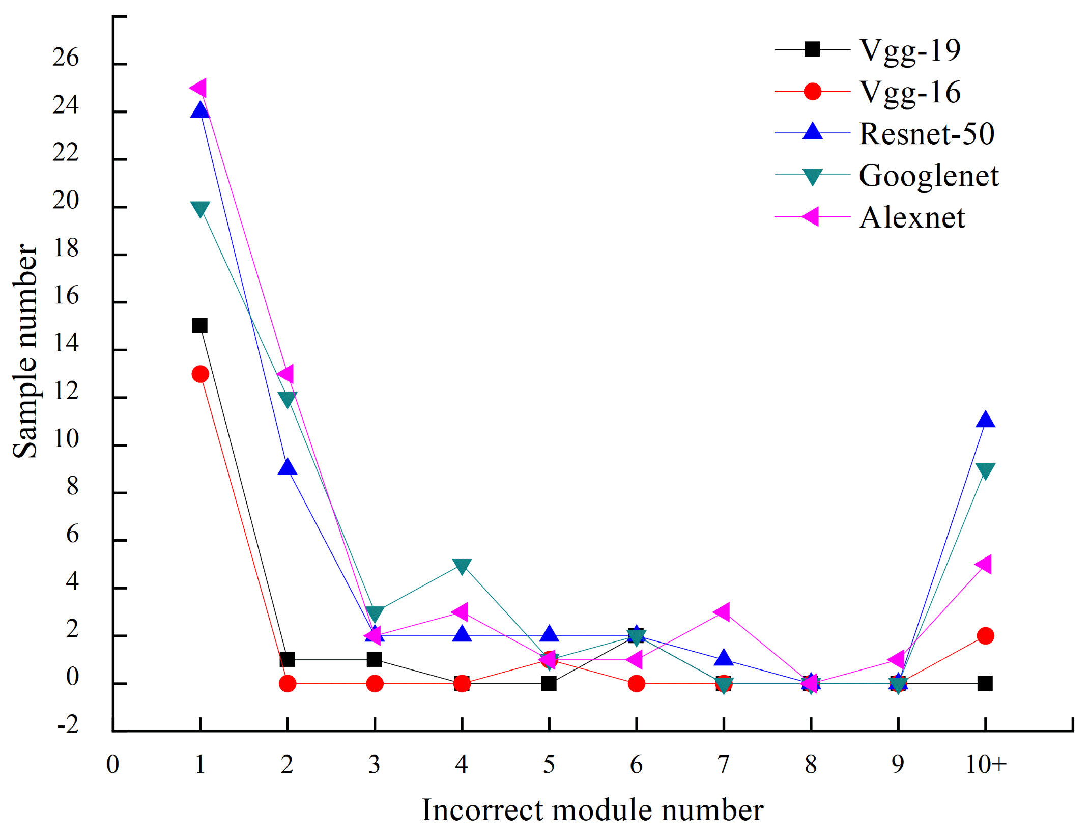
6.3. The Performance of the Proposed Correction Algorithm in the Edge Images
6.4. The Result of Barcode Reconstruction and Recognition
7. Conclusions and Future Work
Author Contributions
Funding
Institutional Review Board Statement
Informed Consent Statement
Data Availability Statement
Acknowledgments
Conflicts of Interest
References
- Xiao, Y.; Ming, Z. 1D barcode detection via integrated deep-learning and geometric approach. Appl. Sci. 2019, 9, 3268. [Google Scholar] [CrossRef] [Green Version]
- Karrach, L.; Pivarčiová, E.; Bozek, P. Recognition of perspective distorted QR codes with a partially damaged finder pattern in real scene images. Appl. Sci. 2020, 10, 7814. [Google Scholar] [CrossRef]
- Kim, J.S.; Yi, C.Y.; Park, Y.J. Image Processing and QR Code Application Method for Construction Safety Management. Appl. Sci. 2021, 11, 4400. [Google Scholar] [CrossRef]
- Nadabar, S.G.; Desai, R. Method and Apparatus Using Intensity Gradients for Visual Identification of 2D Matrix Symbols. U.S. Patent 6,941,026, 6 September 2005. [Google Scholar]
- Che, Z.; Zhai, G.; Liu, J.; Gu, K.; Le Callet, P.; Zhou, J.; Liu, X. A blind quality measure for industrial 2d matrix symbols using shallow convolutional neural network. In Proceedings of the 2018 25th IEEE International Conference on Image Processing (ICIP), Athens, Greece, 7–10 October 2018; pp. 2481–2485. [Google Scholar]
- Liu, X.; Doermann, D.; Li, H. VCode-Pervasive data transfer using video barcode. IEEE Trans. Multimed. 2008, 10, 361–371. [Google Scholar] [CrossRef]
- ISO/IEC-15415; Information Technology-Automatic Identification and Data Capture Techniques-Bar Code Symbol Print Quality Test Specification-Two-Dimensional Symbols. ISO: Geneva, Switzerland, 2011; Volume 2.
- ISO/IEC-16022; Information Technology-Automatic Identification and Data Capture Techniques-Data Matrix Bar Code Symbology Specification. ISO: Geneva, Switzerland, 2006; Volume 2.
- Chen, C.; Kot, A.C.; Yang, H. A two-stage quality measure for mobile phone captured 2D barcode images. Pattern Recognit. 2013, 46, 2588–2598. [Google Scholar] [CrossRef]
- Kang, L.; Ye, P.; Li, Y.; Doermann, D. Convolutional neural networks for no-reference image quality assessment. In Proceedings of the IEEE Conference on Computer Vision and Pattern Recognition, Columbus, OH, USA, 23–28 June 2014; pp. 1733–1740. [Google Scholar]
- Natsukari, C.; Nakata, H. Two-Dimensional Code Reader Setting Method, Two-Dimensional Code Reader, Two Dimensional Code Reader Setting Program and Computer Readable Recording Medium. U.S. Patent 6,983,886, 10 January 2006. [Google Scholar]
- Ottaviani, E.; Pavan, A.; Bottazzi, M.; Brunelli, E.; Caselli, F.; Guerrero, M. A common image processing framework for 2-D barcode reading. IEE Conf. Publ. 1999, 465, 652–655. [Google Scholar]
- Thielemann, J.T.; Schumann-Olsen, H.; Schulerud, H.; Kirkhus, T. Handheld PC with camera used for reading information dense barcodes. In Proceedings of the IEEE Int. Conference on Computer Vision and Pattern Recognition, Demonstration Program, Washington, DC, USA, 27 June–2 July 2004. [Google Scholar]
- Parikh, D.; Jancke, G. Localization and segmentation of a 2D high capacity color barcode. In Proceedings of the 2008 IEEE Workshop on Applications of Computer Vision, Copper Mountain, CO, USA, 7–9 January 2008; pp. 1–6. [Google Scholar]
- Yang, H.; Kot, A.C.; Jiang, X. Binarization of Low-Quality Barcode Images Captured by Mobile Phones Using Local Window of Adaptive Location and Size. IEEE Trans. Image Process. 2011, 21, 418–425. [Google Scholar] [CrossRef] [PubMed]
- Chen, L.; Tang, C.; Xu, M.; Lei, Z. Binarization for low-quality ESPI fringe patterns based on preprocessing and clustering. Appl. Opt. 2021, 60, 9866–9874. [Google Scholar] [CrossRef] [PubMed]
- Sukanthi; Murugan, S.S.; Hanis, S. Binarization of Stone Inscription Images by Modified Bi-level Entropy Thresholding. Fluct. Noise Lett. 2021, 20, 2150054. [Google Scholar] [CrossRef]
- Castellanos, F.J.; Gallego, A.J.; Calvo-Zaragoza, J. Unsupervised neural domain adaptation for document image binarization. Pattern Recognit. 2021, 119, 108099. [Google Scholar] [CrossRef]
- Mukhopadhyay, P.; Chaudhuri, B.B. A survey of Hough Transform. Pattern Recognit. 2015, 48, 993–1010. [Google Scholar] [CrossRef]
- Sun, H.; Uysalturk, M.C.; Karakaya, M. Invisible data matrix detection with smart phone using geometric correction and Hough transform. Opt. Pattern Recognit. XXVII Int. Soc. Opt. Photonics 2016, 9845, 98450P. [Google Scholar] [CrossRef]
- Chelghoum, R.; Ikhlef, A.; Hameurlaine, A.; Jacquir, S. Transfer learning using convolutional neural network architectures for brain tumor classification from MRI images. In IFIP International Conference on Artificial Intelligence Applications and Innovations; Springer: Berlin, Germany, 2020; pp. 189–200. [Google Scholar]
- Krizhevsky, A.; Sutskever, I.; Hinton, G.E. Imagenet classification with deep convolutional neural networks. Adv. Neural Inf. Process. Syst. 2012, 25, 1097–1105. [Google Scholar] [CrossRef]
- Szegedy, C.; Liu, W.; Jia, Y.; Sermanet, P.; Reed, S.; Anguelov, D.; Erhan, D.; Vanhoucke, V.; Rabinovich, A. Going deeper with convolutions. In Proceedings of the IEEE Conference on Computer Vision and Pattern Recognition, Boston, MA, USA, 7–12 June 2015; pp. 1–9. [Google Scholar]
- Simonyan, K.; Zisserman, A. Very deep convolutional networks for large-scale image recognition. arXiv 2014, arXiv:1409.1556. [Google Scholar]
- He, K.; Zhang, X.; Ren, S.; Sun, J. Deep residual learning for image recognition. In Proceedings of the IEEE Conference on Computer Vision and Pattern Recognition, Las Vegas, NV, USA, 27–30 June 2016; pp. 770–778. [Google Scholar]
- Kuhn, H.W. The Hungarian method for the assignment problem. Nav. Res. Logist. Q. 1955, 2, 83–97. [Google Scholar] [CrossRef] [Green Version]
- Munkres, J. Algorithms for the assignment and transportation problems. J. Soc. Ind. Appl. Math. 1957, 5, 32–38. [Google Scholar] [CrossRef] [Green Version]


| ILSVRC Architectures | Number of Layers | Top 5 Error Rate | Training Dataset | Execution Environment |
|---|---|---|---|---|
| AlexNet (2012) | 8 | 15.3% | ImageNet | Two GTX 580 GPUs 3Gg |
| GoogleNet (2014) | 22 | 6.67% | ImageNet | CPU |
| VGGNet (2014) | 16-19 | 6.8% | ImageNet | Four NVIDIA Titan Black GPU |
| ResNet (2015) | 18-34-50-101-152 | 3.57% | ImageNet | Two GPUs |
| Symbol Size | Max Numeric Capacity | Max Alphanumeric Capacity | Max Binary Capacity | Max Correctable Error/Erasure |
|---|---|---|---|---|
| 6 | 3 | 1 | 2 | |
| 10 | 6 | 3 | 3 | |
| 16 | 10 | 6 | 5/7 | |
| 24 | 16 | 10 | 6/9 | |
| 36 | 25 | 20 | 7/11 |
| Type of CNN Models | Total Number of Samples | The Number of Correct Identification | The Number of Incorrect Identification | Accuracy (%) |
|---|---|---|---|---|
| AlexNet | 82,636 | 81,312 | 1324 | 98.4 |
| GoogleNet | 82,636 | 80,899 | 1737 | 97.9 |
| VGG16 | 82,636 | 82,082 | 554 | 99.3 |
| VGG19 | 82,636 | 82,183 | 453 | 99.5 |
| ResNet50 | 82,636 | 81,208 | 1428 | 98.3 |
| Software | The Size of the Set | The Number of Recognized Samples | Recognition Rate (%) |
|---|---|---|---|
| Google ZXing | 200 | 3 | 1.5 |
| Onbarcode.NET | 200 | 10 | 5 |
| Dynamsoft barcode | 200 | 103 | 51.5 |
| LEADTOOLS | 200 | 63 | 31.5 |
| Libdmtx | 200 | 17 | 8.5 |
| Inlite barcode | 200 | 3 | 1.5 |
| Yang [15]+Dynamsoft | 200 | 175 | 78.5 |
| Our solution (four networks) | 200 | >192 | >96.5 |
| our solution (VGG19) | 200 | 199 | 99.5 |
Publisher’s Note: MDPI stays neutral with regard to jurisdictional claims in published maps and institutional affiliations. |
© 2022 by the authors. Licensee MDPI, Basel, Switzerland. This article is an open access article distributed under the terms and conditions of the Creative Commons Attribution (CC BY) license (https://creativecommons.org/licenses/by/4.0/).
Share and Cite
Liao, L.; Li, J.; Lu, C. Data Extraction Method for Industrial Data Matrix Codes Based on Local Adjacent Modules Structure. Appl. Sci. 2022, 12, 2291. https://doi.org/10.3390/app12052291
Liao L, Li J, Lu C. Data Extraction Method for Industrial Data Matrix Codes Based on Local Adjacent Modules Structure. Applied Sciences. 2022; 12(5):2291. https://doi.org/10.3390/app12052291
Chicago/Turabian StyleLiao, Licheng, Jianmei Li, and Changhou Lu. 2022. "Data Extraction Method for Industrial Data Matrix Codes Based on Local Adjacent Modules Structure" Applied Sciences 12, no. 5: 2291. https://doi.org/10.3390/app12052291