Cerebrovascular Segmentation Model Based on Spatial Attention-Guided 3D Inception U-Net with Multi-Directional MIPs

Abstract

The segmentation algorithm of cerebrovascular magnetic resonance angiography (MRA) images based on deep learning plays an essential role in medical study. Traditional segmentation algorithms face poor segmentation results and poor connectivity when the cerebrovascular vessels are thinner. An improved segmentation algorithm based on deep convolutional networks is proposed in this research. The proposed segmentation network combines the original 3D U-Net with the maximum intensity projection (MIP), which was transformed from the corresponding patch of a 3D MRA image. The MRA dataset provided by Jeonbuk National University Hospital was used to evaluate the experimental results in comparison with traditional 3D cerebrovascular segmentation methods and other state–of–the–art deep learning methods. The experimental results showed that our method achieved the best test performance among the compared methods in terms of the Dice score when Inception blocks and attention modules were placed in the proposed dual-path networks.

1. Introduction

The incidence and risk of cerebrovascular diseases are very high, posing a growing threat to human life and health. Early diagnosis and treatment can effectively curb the development of cerebrovascular diseases. The precise segmentation of cerebrovascular diseases is the basis of the auxiliary diagnosis of cerebrovascular diseases. Therefore, cerebrovascular segmentation is of great significance to the auxiliary diagnosis of cerebrovascular diseases and human health. At the same time, cerebrovascular segmentation could reduce the workload of doctors in reading diagnostic images significantly and provide doctors with more accurate disease information.

Nevertheless, compared with traditional organ segmentation, segmenting the cerebrovascular structure from MRA images is extremely challenging due to various difficulties, such as noise, thin or blurred vascular shapes, background noise, and low contrast between the cerebrovascular vessels and the background.

In recent decades, numerous automatic cerebrovascular segmentation methods have been proposed. According to the segmentation principle, the segmentation algorithm of cerebral blood vessels can be divided into three categories: segmentation based on the pixel gray level, based on the vascular tubular structure, and based on experience knowledge.

Segmentation technology based on the pixel gray scale: Because blood vessels are shown as lower gray scales or higher gray scales, different from other tissues in the image, the threshold segmentation method can be used to extract blood vessels. A single fixed value cannot achieve good segmentation. As a result, many researchers have proposed an adaptive threshold segmentation method on this basis. Its principle is based on Shannon information entropy, the Bayes minimum error classification method, fuzzy set theory, or statistical methods. Based on the predecessors, considering that the proportion of blood vessels in the total image information is very small, this easily leads to the maximization algorithm being biased towards the low-gray-value area, resulting in a relatively low threshold and excessive segmentation. Because the maximum intensity projection (MIP) image had a higher proportion of blood vessels than the original image, Gan et al. directly segmented the MIP image of a blood vessel and achieved good results in the inversion of the three-dimensional MRA image, avoiding the phenomenon of excessive segmentation.

Segmentation techniques based on the tubular structure of blood vessels include topology refinement [1,2,3,4] and distance transformation [5,6,7,8]. To obtain an accurate blood vessel model, the tubular structure of the blood vessel is the basis of modeling, and the multi-scale segmentation method [9,10] is based on the eigenvalues of the Hessian matrix. Segmentation technology based on experience knowledge [7,11,12] used a graph-based model to store the prior knowledge of blood vessels in different regions. Under the guidance of this knowledge, the region growing algorithm with an adaptive threshold has been used for segmentation to obtain more accurate results.

Active contour models have been widely applied in image segmentation since the presentation by Kass et al. [13]. However, traditional active contour models can easily converge to incorrect solutions due to the weak constraints. Ding et al. [14] proposed an active contour model that combines region-scalable fitting energy and optimized Laplacian of Gaussian energy for image segmentation. Ref. [15] focused on implicit active contour models and proposed a robust active contour model driven by adaptive functions (including an adaptive edge indicator function and adaptive sign function) and fuzzy c-means energy. Weng et al. [16] proposed an additive bias correction model based on intensity inhomogeneity, and the model divided the observed image into additive bias function, reflection edge structure function, and Gaussian noise. All of these proposed models could obtain an ideal segmentation effect for images with intensity inhomogeneity.

Conventional machine learning typically begins with the machine learning algorithm system computing the image features that are believed to be of importance in making the prediction or diagnosis of interest. More recently, deep learning has started to be used; this method has the benefit that it does not require image feature identification and calculation as a first step; rather, features are identified as part of the learning process.

Research on convolutional neural networks (CNNs) has been emerged and achieved state-of-the-art performance in segmentation tasks [17] over the past thirty years. In medical image processing, there have been several methods based on deep learning to extract blood vessels from 2D images.

The DeepVessel network [18] integrates Conditional Random Field (CRF) into the CNN network, where multi-scale and multi-level CNNs are employed to learn rich hierarchical features. In the 3D vascular scene, Uception [19] integrates the Inception module into the convolutional layer of 3D U-Net [20]. For the sake of reducing the amount of calculations and requiring less GPU memory, 2D orthogonal cross-hair filters are employed to obtain 3D contextual information in DeepVesselNet [21] and VesselNet [22].

Based on the previous work, Yifan Wang et al. proposed a multi-stream CNN framework JointVesselNet [23], which learns 3D features and the corresponding single-direction projection to obtain the 2D MIP features [24,25,26], and then integrates the two into the 3D space. For small blood vessels, better results were achieved.

To further improve the JointVesselNet, we extended the MIP from single-direction to three directions, which increased the amount of information. Furthermore, this paper studies the impact of different loss functions on the segmentation results.

The experimental results are evaluated on our cerebrovascular image dataset; subsequently, a comparison is made between our method and others, including traditional 3D blood vessel segmentation methods and the latest technology in deep learning. Inspired by the representation ability of U-Net [27] and 3D U-Net, in this research, a novel network is adopted for the high-performance cerebrovascular segmentation of MRA images.

The main contributions of this paper include the following:

(1)

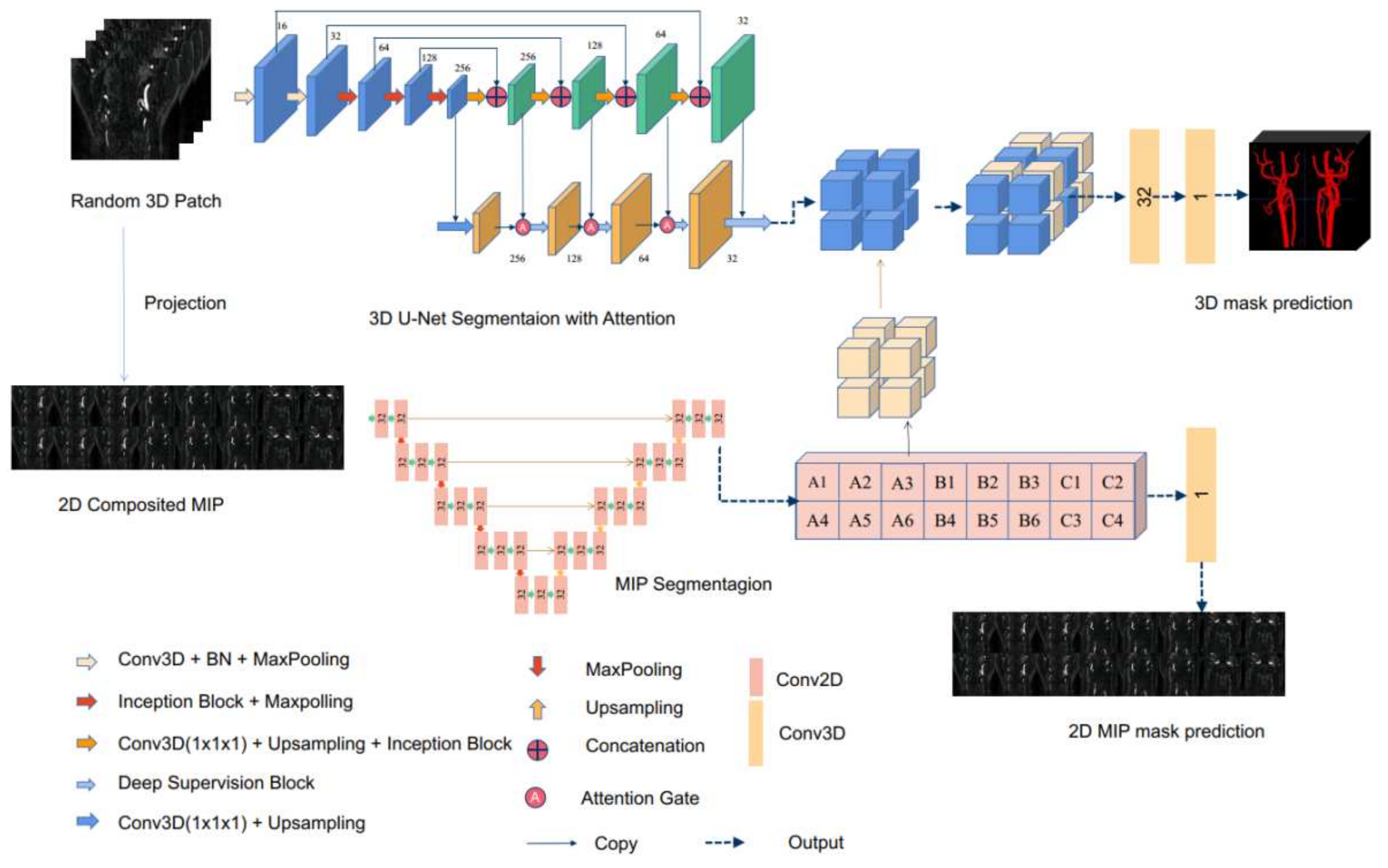
Based on a careful understanding of the network structure of 3D U-Net and the application of MIP to medical images, this paper proposes an improved network using MIP images in three directions to extract richer information. The effectiveness of the improved model is verified by experiments;

(2)

The effect of the loss functions on the segmentation result is studied on the MRA dataset;

(3)

This paper replaces the original convolutional block with the Inception block [28]. In the Inception block, we employ two 3 × 3 filters to obtain an equivalent receptive field of a 5 × 5 convolutional filter, which significantly reduces the amount of computation that has to be done by the network in the subsequent layers.

The remainder of this paper is organized as follows: Section 2 discusses the dataset and the proposed network adopting multi-directional MIP. Section 3 discusses the experimental results, including quantitative and qualitative comparison, along with an ablation study. In Section 4, we end this paper with our conclusions.

2. Materials and Methods

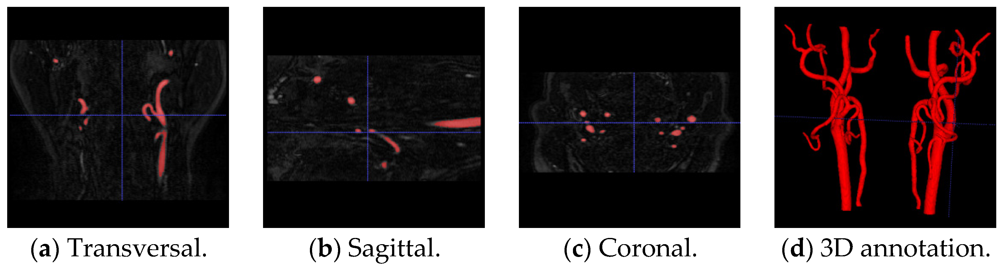
In this section, we describe our experimental dataset and introduce the segmentation model including network architecture, loss function, and metrics.

2.1. Dataset

All patients underwent TOF MR angiography at Jeonbuk National University Hospital. The imaging parameters for the 3D TOF MR angiographic scans were as follows: repetition time (TR)/echo time (TE) = 23 − 25/3.45 ms; flip angle = 20°; field of view (FOV) = 200 × 200 mm; matrix size = 488 × 249; sensitivity encoding (SENSE) factor = 2; slice thickness = 0.50 mm; and number of average (NEX) = 1. The TOF MR angiography scan time was approximately 5.46 min.

To study the possible role of carotid artery anatomy and geometry in the pathogenesis of internal carotid artery (ICA) stenosis [29,30], Jeonbuk National University Hospital collected the patients’ MRA images ten years ago and recently. The dataset contains 64 patients’ cases. The voxel spacing of the MRA images ten years ago is 0.4688 × 0.4688 × 1 mm³, and the volume is 320 × 320 × 200. The voxel spacing of the recent MRA images is 0.3646 × 0.3646 × 0.5000 mm³, and the volume is 960 × 960 × 180 voxels. Data processing personnel use a professional cerebrovascular label software package named ITK-SNAP [31], which is a tool often used to segment anatomical structures. This software provides an automatic active contour segmentation pipeline. By adjusting the active bubbles (including radius and location) and parameters of the contour evolution differential equation in the Snake mode, we could obtain the initial mask; finally, as illustrated in Figure 1, the ground truth cerebrovascular labels are obtained by the domain experts’ post-manual labeling refinement in the paintbrush mode.

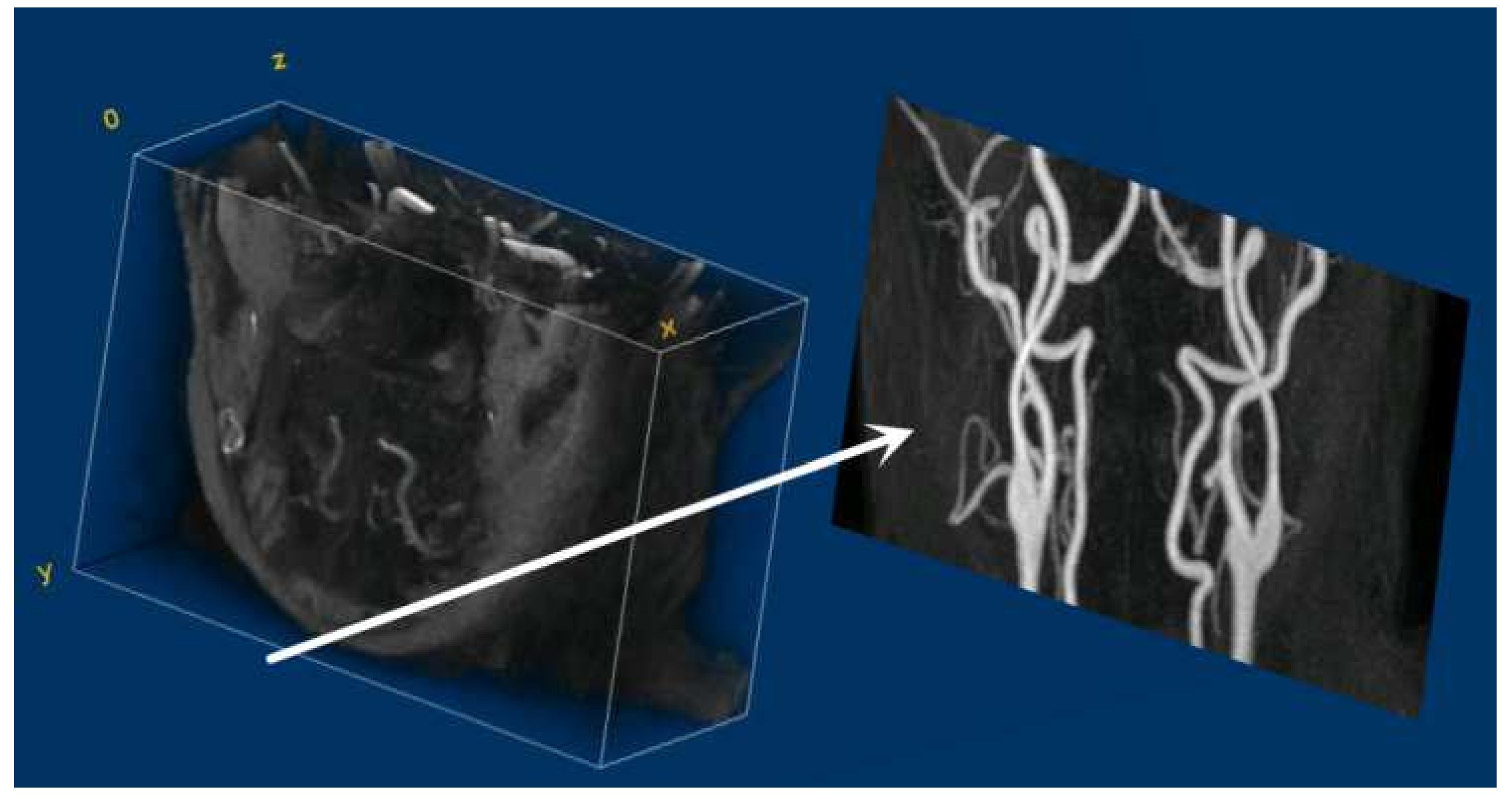
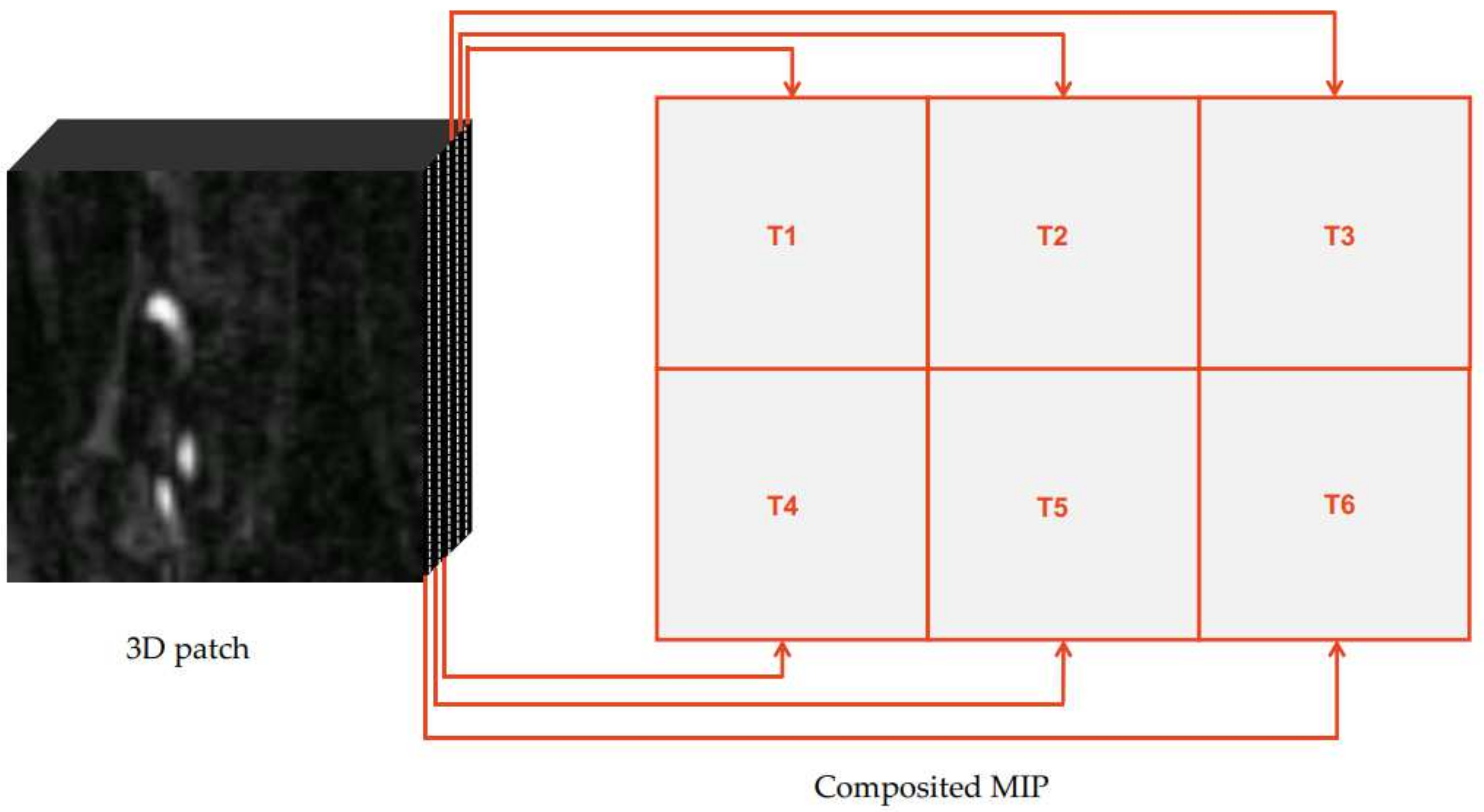
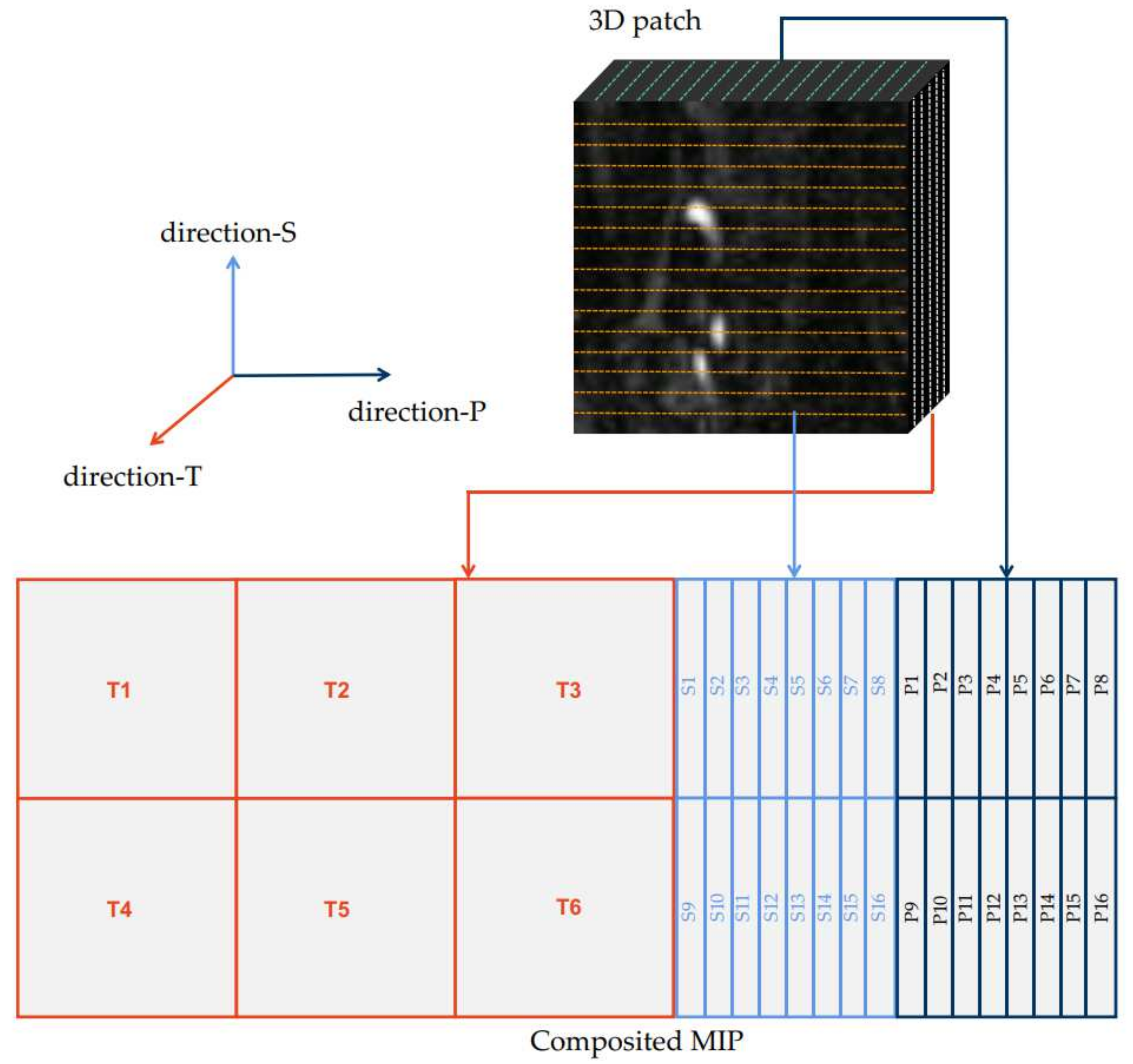
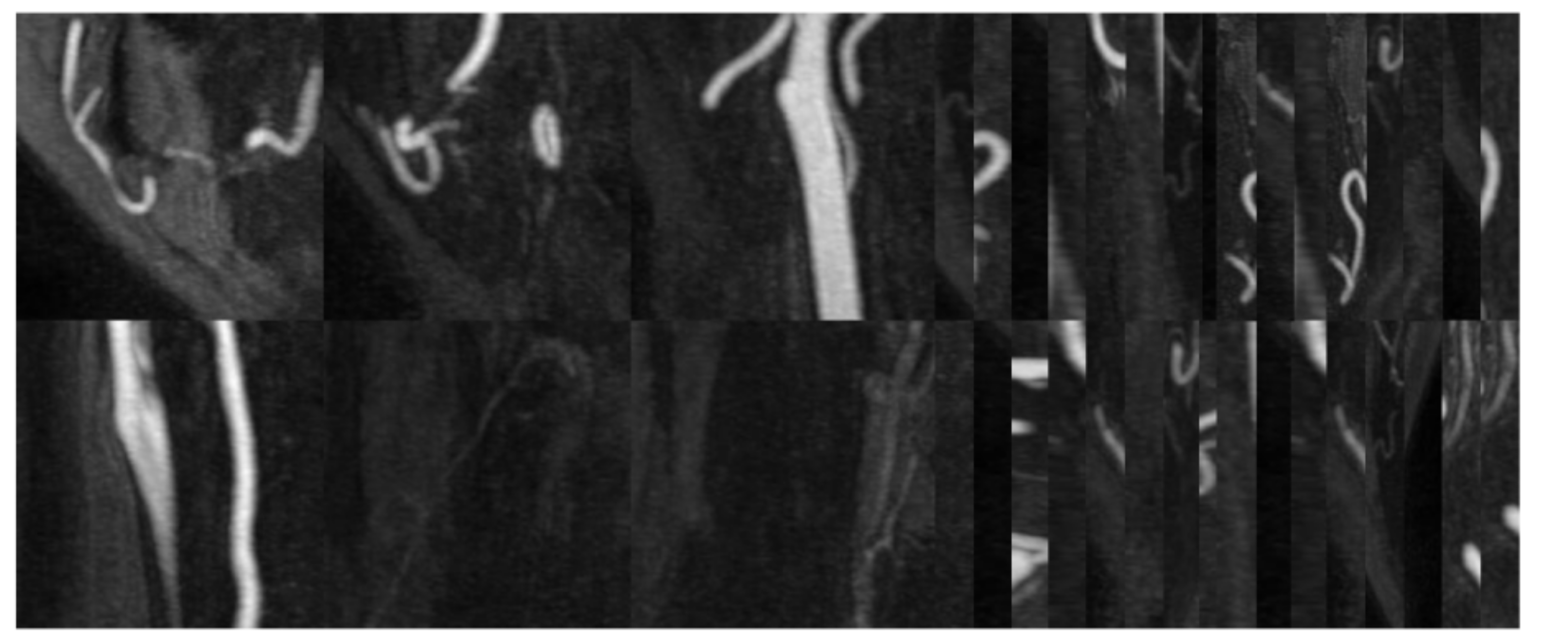
2.2. Multi-Directional MIP

MIP obtains a two-dimensional image by the projection method [24], which is generated by calculating the maximum-density pixels encountered along each ray of the scanned object as illustrated in Figure 2. Despite its simplicity, MIP has been widely adopted in medical image analysis, such as reconstruction [32,33], detection [34,35], and segmentation [36,37,38].

The paper proposing the JointVesselNet [23] applied the idea of MIP to cerebrovascular segmentation. Given a random extraction of a 3D patch of the size K₁ × K₂ × K_3, where K₃ is along the vertical axis, it computes s sliced (s = 6 in the paper) MIPs along the vertical axis. This network aims to enhance the local vessel probability and signal–to–noise ratio by projecting the 3D volume space to the 2D MIP space. As shown in Figure 3, this method divides the 3D image into 6 slices from the volume, and it obtains a composed MIP image by tiling the MIP images coming from each slice, as shown in Figure 3.

It should be noted that only the voxel with the highest intensity in one direction will be recorded in the conventional single-directional 2D MIP in Figure 3. This projection may easily lead to information loss. Considering that the segmentation task requires the information of each voxel, 2D MIP will be too coarse.

Based on this observation, we changed the original single-direction projection to multi-directional projection. In our multi-directional MIP, the volume was divided into s₁, s₂, and s₃ slices from three directions perpendicular to three planes to convey more dense blood vessel information. In our experiment, we used a K₁ × K₂ × K₃ = 128 × 128 × 16 volume patch. We computed s_i slices along each of three axes with overlapping $S_{overlap}$ voxels for consecutive slices. We set $S_{step}$ as the stride. The stride influences the trade-off between information denseness and computation cost. Eventually, we obtained s₁ MIPs of size K₂ × K₃, s₂ MIPs of size K₁ × K₃, and s₃ MIPs of size K₁ × K₂.

$$s_i=\lfloor \frac{K_i - S_{step}}{S_{overlap}}\rfloor +1$$

(1)

In our experiments, we set $S_{step}$ and $S_{overlap}$to 5 and 2, respectively, for $K_3$, and set $S_{step}$ and $S_{overlap}$to 32 and 6, respectively, for $K_1$ and $K_2$. Consequently, the volume was divided into 16, 16, and 6 slices for the three axes. After calculating the corresponding MIP images from each slice, we combined these MIP images into composted MIP images; finally we obtained 2D composite MIP images from the 3D patch (e.g., 38 ( = 16 + 16 + 6) consecutive MIPs). The format of 38 consecutive MIPs is shown in Figure 4. A composted MIP image of one sample patch is shown in Figure 5. The composted MIP image served as the input for the 2D U-Net.

2.3. Network Architecture

The architecture of our proposed network mainly includes two paths, as shown in Figure 6: the upper path sends the 3D image to the 3D U-Net with the attention mechanism for learning, and the lower path projects the 3D image from three directions into the MIP feature vector and sends it to the 2D U-Net. After learning, the 2D MIP feature vector is mapped back to the 3D volume feature space and combined with the 3D feature. The combination of loss functions generated from the two paths is considered as the final loss function of the network.

Because the volume of our blood vessel dataset was relatively large, and the GPU memory limited us to sending images to the network for learning at one time, we randomly selected 100 patches containing valid data from each MRA image and sent each patch to the network. The key to this network was to integrate the learning characteristics of the two paths.

It was observed that, at each layer in the encoder (contraction path), each dimension of the feature map was halved, and the number of feature channels was doubled until the bottleneck was reached. On the other hand, in the decoder (expansion path), each dimension of the feature map was doubled by the up-sampling of the feature dimension to meet the same size as the block to be concatenated in the encoder, and the number of feature channels was halved until the output was reached. In addition, there were long skip connections from the contracting path to the expanding path.

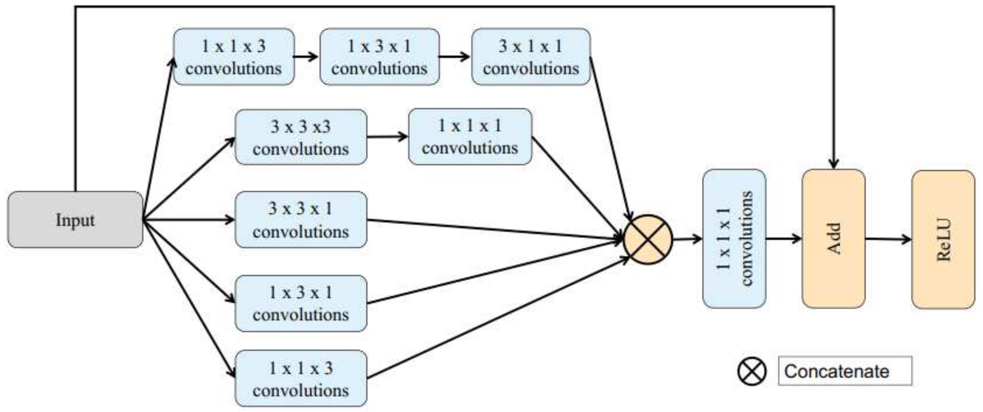
2.3.1. Inception Block

Three-dimensional CNNs are widely employed in various medical image processing tasks, including segmentation and classification [39,40]. Nevertheless, most 3D networks face the challenge of a huge computational burden due to a large number of parameters. Inspired by the idea of Inception V2, we propose a new architecture based on 3D U-Net and decomposed convolutional Inception block [28], in which each convolutional layer in the original U-Net is substituted with an Inception block. A diagram of the proposed Inception block is illustrated in Figure 7.

The Inception block we designed in this paper included several groups of 3D convolution units:

• To extract line-wise features, 1 × 1 × 3, 1 × 3 × 1, and 3 × 1 × 1 convolution units are used;
• To exact 3D features, 3 × 3 × 3 3D convolution units are employed as a supplement, followed by a 1 × 1 × 1 convolution unit, which is used to reduce the number of depth channels and extract point-wise features;
• To extract plane-wise features, 1 × 3 × 3, 3 × 1 × 3, and 3 × 3 × 1 convolution units are introduced;
• A residual structure is added to the Inception block by directly connecting the input to the addition block to accelerate training of network, while the performance is also improved;
• ReLU is employed as the activation function for each layer and batch normalization is performed in each Inception block.

Considering that the size of the decomposed convolution kernel is comparable to the 2D convolution kernel, despite the fact that the depth of the network increases, the parameters of the network do not increase significantly. Our network takes advantage of the efficient Inception blocks in extracting rich features and converges more efficiently.

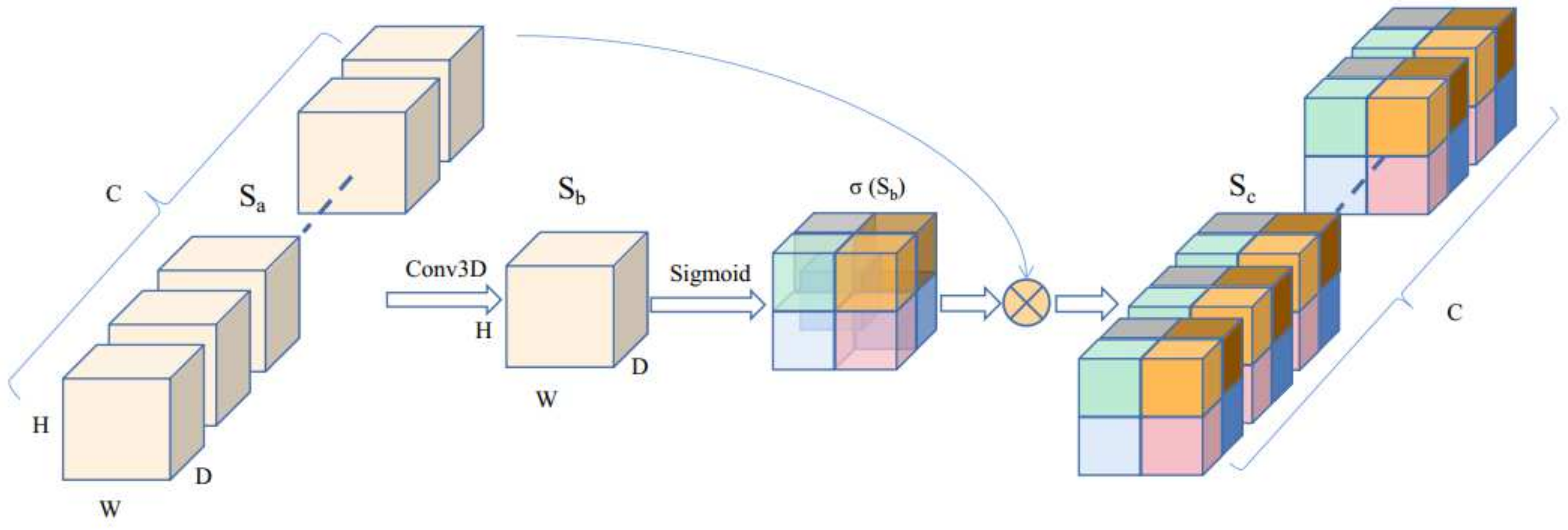
2.3.2. Attention Block

CNNs are the de facto standard for 3D medical image segmentation nowadays because of their high representation ability; U-Net is one of the most effective architectures as this kind of model has a better feature expression ability. Because the shape and size of blood vessels are various in different patients, a U-Net-like architecture relies on multi-level successive convolutional modules, which extract a region of interest (ROI) and perform intensive prediction on this specific ROI. Nevertheless, all modules in the network extract similar low-level features repeatedly; this method often causes redundant use of computing resources. To address this problem, Squeeze–and–Excitation (SE) attention blocks [41,42] are introduced to enhance the accuracy of the segmentation result, which capture spatial correlations between features. For the above-mentioned reasons, we extended the Spatial SE module to a 3D network to compute the channel attention. The architecture of the block is illustrated in Figure 8. We considered the input feature map as follows:

$$S_c=\left[s^{1,1,1,1},s^{1,1,1,2},\dots s^{h,i,j,k},\dots ,s^{C,D,H,W} \right]$$

(2)

where $s^{h,i,j,k}\in ℝ, h\in \left\{1, 2,\dots ,C\right\}, i\in \left\{1, 2,\dots , D\right\}, j\in \left\{1, 2,\dots , H\right\}, k\in \left\{1, 2,\dots , W\right\},$ and h represent the locations of the channels, and i, j, and k represent the spatial location in the direction of the three coordinate axes, respectively. The squeeze operation is employed through a 3D convolution with the output channel of 1, and a projection tensor $S_b\in {ℝ}^{1\times D\times H\times W}$ is generated. This projection tensor is rescaled to [0, 1] through a sigmoid $\sigma$ operation, followed by a spatial multiple operation to excite $S_a$. The definition can be formulated as follows:

$$S_c=\sigma \left(S_a\right)\times S_b$$

(3)

The spatial attention module improves the accuracy of the model by suppressing the activation of features in irrelevant regions for dense label prediction.

2.4. Loss Function and Metrics

Some of the common evaluation metrics for segmentation are the Dice Similarity Coefficient (DSC), Recall (Sensitivity), Specificity, and Precision. The following equations are the mathematical expressions of the abovementioned metrics:

$$DSC\left(A,B\right)=\frac{A\cap B}{A\cup B}=\frac{TP}{TP+FP+FN}$$

(4)

$$Recall=\frac{TP}{TP+FN}$$

(5)

$$Specificity=\frac{TN}{TN+FP}$$

(6)

$$Precision=\frac{TP}{TP+FP}$$

(7)

where TP, FP, and FN are the number of true positive, false positive, and false negative predictions, respectively. Recall is the ratio of true positives to the positives, specificity is the ratio of true negatives to the negatives, and precision is the ratio of true positives to the prediction.

In this paper, three loss functions are applied: Dice loss, Tversky loss, and focal Tversky loss. The dice coefficient is one of the common methods of evaluating the effectiveness of segmentation, and it can also be used as a loss function to measure the similarity of the segmentation and the label:

$$Dice\left(V_p,V_{gt}\right)=\frac{Vox\left(V_p\cap V_{gt}\right)}{Vox\left(V_p\cup V_{gt}\right)}$$

(8)

$$L_{vox\text{-}dice}\left({\delta }_{smoth}\right)=-\frac{2{{\displaystyle \sum }}_{x\in Vox}p\left(x\right)g\left(x\right)+{\delta }_{smoth}}{{{\displaystyle \sum }}_{x\in Vox}p\left(x\right)+{{\displaystyle \sum }}_{x\in Vox}g\left(x\right)+{\delta }_{smoth}}$$

(9)

where $V_p$ represents the voxels’ numbers of the segmentation result, $V_{gt}$ represents voxels’ numbers of ground truth, and $V_p\cap V_{gt}$represents the overlapping voxels of the segmentation result and ground truth. ${\delta }_{smoth}$ is used to avoid division by zero; in our experiment, ${\delta }_{smoth}$ was set to be 1.

There are many data imbalances in medical imaging. The use of imbalanced data for training will lead to a severe bias towards high-precision but low-sensitivity predictions, which is undesirable, especially in medical applications, where false negatives are more likely to be false and positives are more difficult to tolerate. The Tversky loss function solves data imbalance in 3D full deep convolutional neural network training and achieves a good compromise between accuracy and recall.

$$L_{vox\text{-}tversky}\left(\alpha ,{\delta }_{smoth}\right)=-\frac{{{\displaystyle \sum }}_{i\in 1}^N{p}_{0i}{g}_{0i}+{\delta }_{smoth}}{{{\displaystyle \sum }}_{i=1}^N{p}_{0i}{g}_{0i}+\alpha {{\displaystyle \sum }}_{i=1}^N{p}_{0i}{g}_{1i}+\left(1-\alpha \right){{\displaystyle \sum }}_{i=1}^N{p}_{1i}{g}_{1i}+{\delta }_{smoth}}$$

(10)

where ${\delta }_{smoth}$ is used to avoid division by zero; in our experiment, α is set to be 0.7 and ${\delta }_{smoth}$ is set to be 1.

The focal Tversky loss is a generalization form of the Tversky loss. The non-linear feature of the loss helps controlling how the loss behaves at different values of the Tversky index obtained.

$$L_{vox-focal\_tversky}={\left(1-L_{vox-tversky}\right)}^{\mathsf{\gamma }}$$

(11)

where γ is a parameter that controls the non-linearity of the loss. As γ tends to positive ∞, the gradient of the loss tends to ∞ as the Tversky Index tends to 1. As γ tends to 0, the gradient of the loss tends to 0 as Tversky Index tends to 1. In our experiment, γ is set to be 0.75.

Inspired by the idea of the focal loss to address the class imbalance problem, our final loss consists of loss from two paths; the loss from each path is based on the three loss functions described above, and the final loss defined as:

$$L=L_{vox}+\mathsf{\lambda }{L}_{mip}$$

(12)

where λ represents the weight between the two losses, which was set to be 0.25 for our best experiment performance.

3. Experiment and Results

3.1. Experiments

3.1.1. Data Pre-Processing and Augmentation

A pre-processing method was applied to the input data before feeding the data into our network. Since the MRA values were non-standardized, we applied Z-score normalization to each MRA image from each patient; Z-score normalization uses the cerebrovascular mask for the image I(x) to determine the mean ${\mu }_{z\text{-}score}$ and standard deviation σ_z-score of the intensities inside the brain mask. The formula for the Z-score-normalized image is below:

$$L_{z\text{-}score}\left(x\right)=-\frac{I\left(x\right)-{\mu }_{z\text{-}score}}{{\mathsf{\sigma }}_{z\text{-}score}}$$

(13)

where I(x) represents the input image, ${\mu }_{z\text{-}score}$ is the mean value of the feature, and σ_z-score is the standard deviation of the feature.

Furthermore, we applied two types of data augmentation to the input data to avoid an overfitting issue:

• We cropped the MRA image randomly from 320 × 320 × 200 or 960 × 960 × 180 voxels to 128 × 128 × 16 voxels to train our network due to memory limitation. For each volume, 100 patches were randomly extracted. For example, there were 64 cases in the dataset, and we obtained 6400 patches for training after extracting;
• We flipped along each 3D axis randomly with a probability of 0.5.

3.1.2. Training Details

All 6400 patches were split into training/validation/test sets in a ratio of 6:2:2. Hence, we could obtain random training/validation/test cases, respectively, as 2400/1280/1280.

The maximum number of training iterations was set to 85 and the Adam optimizer was employed to update the weights of the network, with a batch size of 1 and an initial learning rate of 0.0001. The linear warming-up policy [43] was adopted to start the training; the warm-up ratio and learning decay rate were set to 0.1 and 0.5, respectively.

Inspired by stochastic weights averaging (SWA), we employed the SWA method in training our network. To obtain more robust predictions, after the initial 85 epoch training, we further trained it for another 12 epochs and then averaged these 12 checkpoints as our final model.

3.1.3. Post-Processing

We performed the following methods to post-process the predicted cerebrovascular:

• Noisy pixels on borders or further away from the main volume were removed by eroding operations;
• The surfaces of the predicted result were smoothed by the smoothing operator;
• Holes inside the cerebrovascular segmentation result were removed by removing the connected domains with smaller volumes.

Training was performed on a GeForce GTX 2080Ti GPU with 11G memory. We used eight GPUs for training with a total batch size of eight (one patch per GPU) in the performance comparison and ablation study.

3.2. Quantitative Comparison

We first investigated the effect of the hyper-parameter λ of the loss in Equation (12) on the segmentation performance.

Table 1. Performance of the network when changing the hyper-parameter (λ) of our loss.

λ	DSC	Recall	Specificity	Precision
0.15	92.40	86.34	99.96	92.82
0.25	93.84	91.35	99.96	93.92
0.35	93.68	88.60	99.96	93.86
...	...	...	...	...
0.90	68.02	70.22	99.86	75.35

shows the performance of the network when varying λ from 0.1 to 0.9. λ = 0.25 worked best (93.84 Dice, 93.92 Precision), and we adopted this value for all of the following experiments.

We compared our network performance on the MRA dataset to seven advanced deep learning-based methods (e.g., Vesselness, DeepVessel, DeepVesselNet, Uception, 2D U-Net, 3D U-Net, and JointVesselNet). The same dataset split was used in all of these deep-learning methods for a fair comparison.

Two quantitative indicators were applied, namely dice similarity (Dice) and precision, for quantitative performance evaluation. For fairness, the same pre-processing and post-processing were applied to every model. The performance comparison of different methods on the MRA dataset is shown in Table 1. The best results in the table are shown in bold. As shown in

Table 2. Quantitative performance evaluation of different methods.

Network	DSC	Recall	Specificity	Precision
VesselNet [22]	73.29	72.51	99.92	75.36
DeepVessel [18]	82.61	81.49	99.94	84.26
DeepVesselNet [21]	84.59	82.62	99.94	85.18
2D U-Net [27]	87.48	85.31	99.94	89.54
3D U-Net [20]	90.43	88.60	99.96	90.49
JointVesselNet [23]	92.82	90.13	99.96	92.95
Ours	93.84	91.35	99.96	93.92

, our proposed network had the best overall performance among the compared methods applied to the dataset.

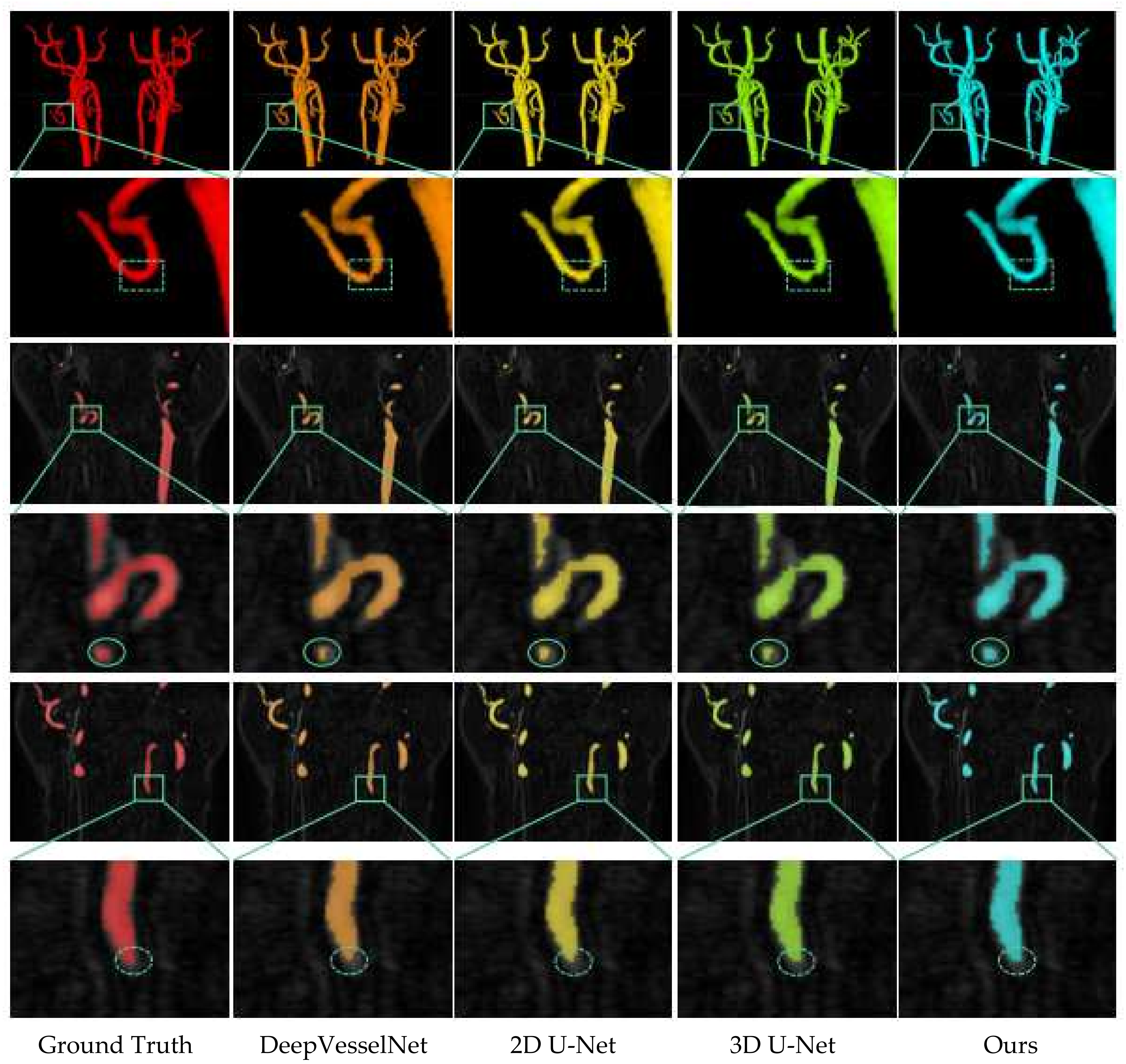
3.3. Qualitative Comparison

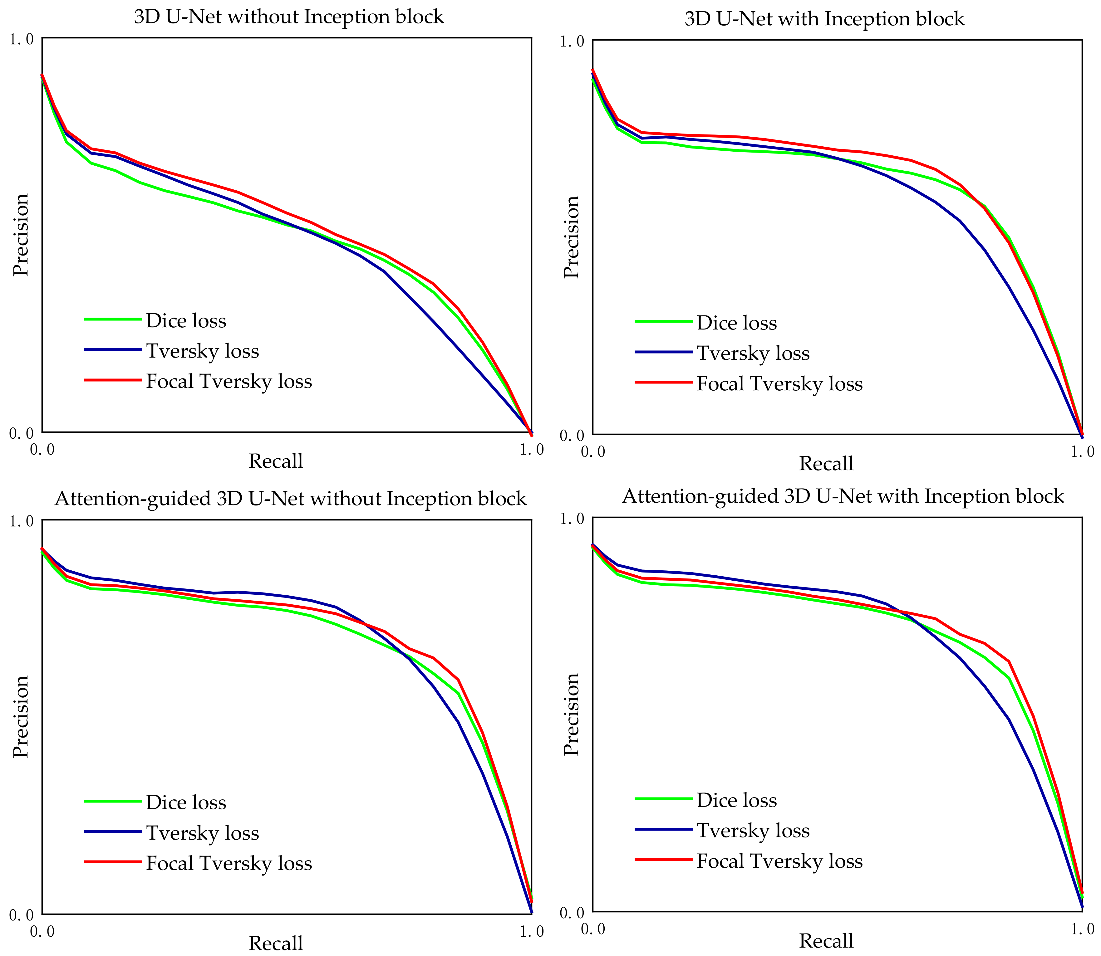
As shown in Figure 9, the segmentation results still cannot remove position-related interference, such as the end of the cerebrovascular vessels (green dotted ellipse in the sixth row); all methods, including ours, could not obtain accurate segmentation at the end of the cerebrovascular vessel. The experimental results show that our numerical evaluation is superior to the other methods in all indicators.

From the 3D visualization in the second row, our cerebrovascular segmentation shows better connectivity (near narrow and tortuous portion), as marked in the green dotted rectangle; other segmentation methods had varying degrees of deficiency in narrow areas, among which DeepVesselNet and 2D U-Net achieved the worst performance.

From the figure in the fourth row, our cerebrovascular segmentation showed better ability to capture small blood vessels compared to the other methods, as marked in the green solid ellipse; 2D U-Net also achieved good performance, however, some pixels could not be segmented correctly in the DeepVesselNet and 3D U-Net methods.

This result shows that our cerebrovascular segmentation method achieved more continuous and clearer results than those obtained by other methods.

3.4. Ablation Study

To further test the role of the Inception block, attention module, and different loss functions, we conducted the following series of ablation experiments. From the experimental results in

Table 3. Comparison of the use of the Inception block and Attention mechanism and different loss functions.

Network	AttentionMechanism	Loss Function	Dice (%)
3D U-Net	Without attention	Dice Loss	93.63
		Tversky Loss	92.15
		Focal Tversky Loss	93.06
	With attention	Dice Loss	93.69
		Tversky Loss	92.25
		Focal Tversky Loss	93.43
3D U-Net (Inception block)	Without attention	Dice Loss	93.67
		Tversky Loss	92.65
		Focal Tversky Loss	93.77
	With attention	Dice Loss	93.71
		Tversky Loss	93.78
		Focal Tversky Loss	93.84

, we used the Inception block instead of the original 3D U-Net convolution block, and the attention mechanism could achieve better results; in the Loss Function test, using focal Tversky loss could achieve better results.

4. Discussion

With our proposed model based on spatial attention-guided 3D Inception U-Net with multi-directional MIPs, we achieved an improved precision–recall trade-off and a high DSC of 93.84, which is better than that of other methods. The JointVesselNet model achieved a DSC of 92.82, and the 3D U-Net model achieved a DSC of 90.43. We achieved improved performance by using our architecture together with the Focal Tversky loss.

The experimental results in MRA segmentation showed that all performance evaluation metrics were improved by using the Focal Tversky loss function, rather than using the Dice similarity coefficient loss or Tversky loss in the loss layer.

The specificity metric was always very high (e.g., ≥99%) in the highly unbalanced data of the MRA images; to critically evaluate the performance of the segmentation for the highly unbalanced dataset, we used the Precision–Recall (PR) curve as well as the area under the PR curve (APR, shown in Figure 10), the most reliable performance metric for such highly unbalanced data.

5. Conclusions

In this research, an improved convolutional network based on 3D U-Net and MIP is proposed for the cerebrovascular segmentation of MRA images. The proposed network mainly consists of a dual-stream component, which included a spatial attention-guided 3D Inception U-Net segmentation stream and a 2D composited multi-directional MIPs U-Net segmentation stream.

By combining the features of the 2D MIP feature vectors of three directions with 3D features, the proposed network considers both large blood vessels and small blood vessels, as well as has better vessel connectivity. By studying the loss function and replacing the convolutional block with the Inception block, we further improved the accuracy of cerebrovascular segmentation and reduced the computational amount. The effectiveness of our method was evaluated on a dataset with 64 volumes obtained from 64 patients. The experimental results demonstrated that the model proposed in this research provided better results on cerebrovascular segmentation, achieving state–of–the–art performance in the existing methods.

One shortcoming of our proposed model is that the segmentation results obtained at the end of cerebrovascular vessels did not perform well. In future work, we will consider a cascaded model, which addresses this practical drawback of 3D U-Net’s poor segmentation results on details. Considering the outstanding performance of the nnU-Net [44] model in medical image segmentation, a 3D U-Net is first trained on down-sampled images, and the segmentation results of this U-Net are then up-sampled to the original voxel spacing and passed as additional input channels to a second 3D U-Net, which is trained on patches at full resolution. We may study and apply cascaded models to our future research.

References

1. Bi, J. A Novel Thinning Algorithm of 3D Image Model Based on Spatial Wavelet Interpolation. J. Comput. 2013, 8, 3012–3019. [Google Scholar] [CrossRef] [Green Version]
2. Pujari, A.K.; Mitra, C.; Mishra, S. A new parallel thinning algorithm with stroke correction for odia characters. In Advanced Computing, Networking and Informatics-Volume 1; Springer: Berlin/Heidelberg, Germany, 2014; pp. 413–419. [Google Scholar]
3. Kwon, J.-S. Improved parallel thinning algorithm to obtain unit-width skeleton. Int. J. Multimed. Appl. 2013, 5, 1–14. [Google Scholar] [CrossRef]
4. Gayathri, S.; Sridhar, V. An improved fast thinning algorithm for fingerprint image. Int. J. Eng. Sci. Innov. Technol. 2013, 2, 264–270. [Google Scholar]
5. Fabbri, R.; Costa, L.D.F.; Torelli, J.C.; Bruno, O.M. 2D Euclidean distance transform algorithms: A comparative survey. ACM Comput. Surv. 2008, 40, 1–44. [Google Scholar] [CrossRef]
6. Gurumoorthy, K.S.; Rangarajan, A. Distance Transform Gradient Density Estimation Using the Stationary Phase Approximation. SIAM J. Math. Anal. 2012, 44, 4250–4273. [Google Scholar] [CrossRef]
7. Rong, G.; Tan, T.-S. Jump flooding in GPU with applications to Voronoi diagram and distance transform. In Proceedings of the 2006 Symposium on Interactive 3D Graphics and Games, Redwood City, CA, USA, 14–17 March 2006; pp. 109–116. [Google Scholar]
8. Breu, H.; Gil, J.; Kirkpatrick, D.; Werman, M. Linear-Time Euclidean Distance Transform Algorithms. IEEE Trans. Pattern Anal. Mach. Intell. 1995, 17, 529–533. [Google Scholar] [CrossRef]
9. Olabarriaga, S.D.; Breeuwer, M.; Niessen, W. Evaluation of Hessian-Based Filters to Enhance the Axis of Coronary Arteries in CT Images; International Congress Series; Elsevier: Amsterdam, The Netherlands, 2003; pp. 1191–1196. [Google Scholar]
10. Truc, P.T.H.; Khan, M.A.U.; Lee, Y.K.; Lee, S.; Kim, T.S. Vessel enhancement filter using directional filter bank. Comput. Vis. Image Underst. 2009, 113, 101–112. [Google Scholar] [CrossRef]
11. Faber, S.C.; Hoffmann, A.; Ruedig, C.; Reiser, M. MRI-induced stimulation of peripheral nerves: Dependency of stimulation threshold on patient positioning. Magn. Reson. Imaging 2003, 21, 715–724. [Google Scholar] [CrossRef]
12. Passat, N.; Ronse, C.; Baruthio, J.; Armspach, J.P.; Foucher, J. Watershed and multimodal data for brain vessel segmentation: Application to the superior sagittal sinus. Image Vis. Comput. 2007, 25, 512–521. [Google Scholar] [CrossRef] [Green Version]
13. Kass, M.; Witkin, A.; Terzopoulos, D. Snakes: Active contour models. Int. J. Comput. Vis. 1988, 1, 321–331. [Google Scholar] [CrossRef]
14. Ding, K.; Xiao, L.; Weng, G. Active contours driven by region-scalable fitting and optimized Laplacian of Gaussian energy for image segmentation. Signal Process. 2017, 134, 224–233. [Google Scholar] [CrossRef]
15. Jin, R.; Weng, G. Active contours driven by adaptive functions and fuzzy c-means energy for fast image segmentation. Signal Process. 2019, 163, 1–10. [Google Scholar] [CrossRef]
16. Weng, G.; Dong, B.; Lei, Y. A level set method based on additive bias correction for image segmentation. Expert Syst. Appl. 2021, 185, 115633. [Google Scholar] [CrossRef]
17. Kayalibay, B.; Jensen, G.; van der Smagt, P. CNN-based segmentation of medical imaging data. arXiv 2017, arXiv:1701.03056. [Google Scholar]
18. Fu, H.; Xu, Y.; Lin, S.; Wong, D.W.K.; Liu, J. Deepvessel: Retinal vessel segmentation via deep learning and conditional random field. In Proceedings of the International Conference on Medical Image Computing and Computer-Assisted Intervention, Athens, Greece, 17–21 October 2016; Springer: Berlin/Heidelberg, Germany, 2016; pp. 132–139. [Google Scholar]
19. Sanchesa, P.; Meyer, C.; Vigon, V.; Naegel, B. Cerebrovascular network segmentation of MRA images with deep learning. In Proceedings of the 2019 IEEE 16th International Symposium on Biomedical Imaging (ISBI 2019), Venice, Italy, 8–11 April 2019; IEEE: Piscataway, NJ, USA, 2019; pp. 768–771. [Google Scholar]
20. Çiçek, Ö.; Abdulkadir, A.; Lienkamp, S.S.; Brox, T.; Ronneberger, O. 3D U-Net: Learning dense volumetric segmentation from sparse annotation. In Proceedings of the International Conference on Medical Image Computing and Computer-Assisted Intervention, Athina, Greece, 17–21 October 2016; Springer: Berlin/Heidelberg, Germany, 2016; pp. 424–432. [Google Scholar]
21. Tetteh, G.; Efremov, V.; Forkert, N.D.; Schneider, M.; Kirschke, J.; Weber, B.; Zimmer, C.; Piraud, M.; Menze, B.H. DeepVesselNet: Vessel Segmentation, Centerline Prediction, and Bifurcation Detection in 3-D Angiographic Volumes. Front. Neurosci. 2020, 14, 592352. [Google Scholar] [CrossRef]
22. Wu, Y.; Xia, Y.; Song, Y.; Zhang, D.; Liu, D.; Zhang, C.; Cai, W. Vessel-Net: Retinal vessel segmentation under multi-path supervision. In Proceedings of the International Conference on Medical Image Computing and Computer-Assisted Intervention, Shenzhen, China, 13–17 October 2019; Springer: Berlin/Heidelberg, Germany, 2019; pp. 264–272. [Google Scholar]
23. Wang, Y.; Yan, G.; Zhu, H.; Buch, S.; Wang, Y.; Haacke, E.M.; Hua, J.; Zhong, Z. JointVesselNet: Joint Volume-Projection Convolutional Embedding Networks for 3D Cerebrovascular Segmentation. In Proceedings of the International Conference on Medical Image Computing and Computer-Assisted Intervention, Istanbul, Turkey, 4–8 October 2020; Springer: Berlin/Heidelberg, Germany, 2020; pp. 106–116. [Google Scholar]
24. Prokop, M.; Shin, H.O.; Schanz, A.; SchaeferProkop, C.M. Use of maximum intensity projections in CT angiography: A basic review. Radiographics 1997, 17, 433–451. [Google Scholar] [CrossRef]
25. Angermann, C.; Haltmeier, M. Random 2.5 d u-net for fully 3d segmentation. In Machine Learning and Medical Engineering for Cardiovascular Health and Intravascular Imaging and Computer Assisted Stenting; Springer: Berlin/Heidelberg, Germany, 2019; pp. 158–166. [Google Scholar]
26. Angermann, C.; Haltmeier, M.; Steiger, R.; Pereverzyev, S.; Gizewski, E. Projection-based 2.5 d u-net architecture for fast volumetric segmentation. In Proceedings of the 2019 13th International Conference on Sampling Theory and Applications (SampTA), Bordeaux, France, 8–12 July 2019; IEEE: Piscataway, NJ, USA, 2019; pp. 1–5. [Google Scholar]
27. Ronneberger, O.; Fischer, P.; Brox, T. U-net: Convolutional networks for biomedical image segmentation. In Proceedings of the International Conference on Medical Image Computing and Computer-Assisted Intervention, Munich, Germany, 5–9 October 2015; Springer: Berlin/Heidelberg, Germany, 2015; pp. 234–241. [Google Scholar]
28. Szegedy, C.; Ioffe, S.; Vanhoucke, V.; Alemi, A.A. Inception-v4, inception-resnet and the impact of residual connections on learning. In Proceedings of the Thirty-First AAAI Conference on Artificial Intelligence, San Francisco, CA, USA, 4–9 February 2017. [Google Scholar]
29. Jeon, S.J.; Kwak, H.S.; Chung, G.H. Widening and Rotation of Carotid Artery with Age: Geometric Approach. J Stroke Cereb. Dis 2018, 27, 865–870. [Google Scholar] [CrossRef]
30. Jeong, S.K.; Lee, J.H.; Nam, D.H.; Kim, J.T.; Ha, Y.S.; Oh, S.Y.; Park, S.H.; Lee, S.H.; Hur, N.; Kwak, H.S.; et al. Basilar artery angulation in association with aging and pontine lacunar infarction: A multicenter observational study. J. Atheroscler. Thromb. 2015, 22, 509–517. [Google Scholar] [CrossRef] [Green Version]
31. Yushkevich, P.A.; Gao, Y.; Gerig, G. ITK-SNAP: An interactive tool for semi-automatic segmentation of multi-modality biomedical images. In Proceedings of the 2016 38th Annual International Conference of the IEEE Engineering in Medicine and Biology Society (EMBC), Orlando, FL, USA, 16–20 August 2016; IEEE: Piscataway, NJ, USA, 2016; pp. 3342–3345. [Google Scholar]
32. Marquis, H.; Deidda, D.; Gillman, A.; Willowson, K.; Gholami, Y.; Hioki, T.; Eslick, E.; Thielemans, K.; Bailey, D. Theranostic SPECT Reconstruction for Improved Lesion Dosimetry in Radionuclide Therapy. J. Nucl. Med. 2021, 62 (Suppl. 1), 1533. [Google Scholar]
33. Li, S.; Zhao, Y.; Ye, Y. Improved minimum intensity projection in holographic reconstruction via SNR-enhanced holography. J. Mod. Opt. 2021, 68, 322–326. [Google Scholar] [CrossRef]
34. Kawel, N.; Seifert, B.; Luetolf, M.; Boehm, T. Effect of Slab Thickness on the CT Detection of Pulmonary Nodules: Use of Sliding Thin-Slab Maximum Intensity Projection and Volume Rendering. Am. J. Roentgenol. 2009, 192, 1324–1329. [Google Scholar] [CrossRef]
35. Fujii, S.; Matsusue, E.; Kanasaki, Y.; Kanamori, Y.; Nakanishi, J.; Sugihara, S.; Kigawa, J.; Terakawa, N.; Ogawa, T. Detection of peritoneal dissemination in gynecological malignancy: Evaluation by diffusion-weighted MR imaging. Eur. Radiol. 2008, 18, 18–23. [Google Scholar] [CrossRef] [PubMed]
36. Wang, H.; Yao, D.; Chen, J.; Liu, Y.; Li, W.; Shi, Y. 2d–3d Hierarchical Feature Fusion Network For Segmentation Of Bone Structure In Knee Mr Image. In Proceedings of the 2021 IEEE 18th International Symposium on Biomedical Imaging (ISBI), Nice, France, 13–16 April 2021; IEEE: Piscataway, NJ, USA, 2021; pp. 575–578. [Google Scholar]
37. Jadhav, S.; Deng, G.; Zawin, M.; Kaufman, A.E. COVID-view: Diagnosis of COVID-19 using Chest CT. IEEE Trans. Vis. Comput. Graph. 2021. [CrossRef] [PubMed]
38. Yousefirizi, F.; Martineau, P.; Uribe, C.; Rahmim, A. Enhancement of conventional segmentation techniques to achieve deep framework performance for lymphoma lesion segmentation in PET images. J. Nucl. Med. 2021, 62 (Suppl. 1), 1427. [Google Scholar]
39. Szegedy, C.; Vanhoucke, V.; Ioffe, S.; Shlens, J.; Wojna, Z. Rethinking the inception architecture for computer vision. In Proceedings of the IEEE Conference on Computer Vision and Pattern Recognition, Las Vegas, NV, USA, 27–30 June 2016; IEEE: Piscataway, NJ, USA, 2016; pp. 2818–2826. [Google Scholar]
40. Qi, C.R.; Su, H.; Mo, K.; Guibas, L.J. Pointnet: Deep learning on point sets for 3d classification and segmentation. In Proceedings of Proceedings of the IEEE Conference on Computer Vision and Pattern Recognition, Honolulu, HI, USA, 21–26 July 2017; IEEE: Piscataway, NJ, USA, 2017; pp. 652–660. [Google Scholar]
41. Woo, S.; Park, J.; Lee, J.-Y.; Kweon, I.S. Cbam: Convolutional block attention module. In Proceedings of the European conference on computer vision (ECCV), Munich, Germany, 8–14 September 2018; pp. 3–19. [Google Scholar]
42. Oktay, O.; Schlemper, J.; Folgoc, L.L.; Lee, M.; Heinrich, M.; Misawa, K.; Mori, K.; McDonagh, S.; Hammerla, N.Y.; Kainz, B. Attention u-net: Learning where to look for the pancreas. arXiv 2018, arXiv:1804.03999. [Google Scholar]
43. He, T.; Zhang, Z.; Zhang, H.; Zhang, Z.; Xie, J.; Li, M. Bag of tricks for image classification with convolutional neural networks. In Proceedings of the IEEE/CVF Conference on Computer Vision and Pattern Recognition, Long Beach, CA, USA, 15–20 June 2019; IEEE: Piscataway, NJ, USA, 2019; pp. 558–567. [Google Scholar]
44. Isensee, F.; Petersen, J.; Klein, A.; Zimmerer, D.; Jaeger, P.F.; Kohl, S.; Wasserthal, J.; Koehler, G.; Norajitra, T.; Wirkert, S. Nnu-net: Self-adapting framework for u-net-based medical image segmentation. arXiv 2018, arXiv:1809.10486. [Google Scholar]
Figure 1. The cerebrovascular vessels of interest are labeled in red in every plane (ac). The corresponding 3D segmentation masks are shown in (d).
Applsci 12 02288 g001
Figure 2. Basic principle of single-directional MIP obtaining maximum intensity along each ray during the projection of the 3D volume patch to a 2D MIP image along the direction indicated by the arrow.
Applsci 12 02288 g002
Figure 3. Composed MIP images coming from each of s slices (s = 6 in this example).
Applsci 12 02288 g003
Figure 4. Illustration of the proposed multi-directional MIP.
Applsci 12 02288 g004
Figure 5. Composed MIP images of the sample patch.
Applsci 12 02288 g005
Figure 6. The architecture of our proposed network.
Applsci 12 02288 g006
Figure 7. The architecture of the Inception block.
Applsci 12 02288 g007
Figure 8. The architecture of the Attention Block.
Applsci 12 02288 g008
Figure 9. Some qualitative comparison.
Applsci 12 02288 g009
Figure 10. PR curves with different losses for all test sets obtained by the four examined approaches. The best results based on the precision–recall trade-off were always obtained with the Focal Tversky loss function.
Applsci 12 02288 g010