oneM2M-Enabled Prediction of High Particulate Matter Data Based on Multi-Dense Layer BiLSTM Model

Abstract

High particulate matter (PM) concentrations in the cleanroom semiconductor factory have become a significant concern as they can damage electronic devices during the manufacturing process. PM can be predicted before becoming more concentrated based on its historical data to support factory management in regulating the air quality in the cleanroom. In this paper, a Multi-Dense Layer BiLSTM model is proposed to predict PM2.5 concentrations in the indoor environment of the cleanroom. To obtain reliability, validity, and interoperability data, the datasets containing temperature, humidity, PM0.3, PM0.5, PM1, PM2.5, PM5, and PM10 were retrieved in a standardized manner via oneM2M-defined representational state transfer application programmable interfaces by employing software platforms compliant with the Internet of Things (IoT) standard. Based on the proposed model, an algorithm was built providing short-term PM2.5 concentration predictions (one hour ahead, two hours ahead, and three hours ahead). The proposed model outperformed the RNN, LSTM, CNN-LSTM, and Single-Dense Layer BiLSTM models in terms of MSE, MAE, and MAPE values. The model created in this study could predict high PM2.5 concentration levels more accurately, thus providing vital support for operation and maintenance for the semiconductor industry.

1. Introduction

The semiconductor industry is one of the world’s most rapidly growing and evolving industries. The global semiconductor market is estimated to be worth 333 billion dollars. In addition, the industry has a considerable impact on the national market economy, accounting for 10–15% of the Republic of Korea’s total exports. Market competition is becoming increasingly vital due to the recent growth of available electronic gadgets, such as mobile phones and tablet PCs (personal computers) [1]. Semiconductor fabrication requires a variety of complex chemical components [2], generating various chemicals and by-products that are almost impossible to remove from the inside of the equipment altogether. Powders and airborne PM, the by-products of the chemical reaction of the metal precursors used as process materials during regular operation and their release into the workplace during process equipment and scrubber maintenance (used to remove some particulates and gases from industrial exhaust streams), can severely damage the electronic circuits [3].

The yield of the semiconductor industry is defined as the percentage of functional integrated circuit (IC) devices at the end of the fabrication process. In general, there are two types of yield losses in IC manufacturing: systematic and random yield loss. Deviations in the device and material characteristics cause systematic yield loss. Contamination issues and process-induced particles are frequently linked to random defect yield loss [4]. The following are a few instances of contaminations and mechanisms responsible for the electronic chip failures in a semiconductor: particulate matter contamination, either from organic or inorganic matter particles created by the environment or by tools, and processes, such as scratches, fractures, overlay flaws, and stress [5]. As a result, in industrial hygiene, monitoring, determining, and predicting the powder by-products and airborne PM in the cleanroom semiconductor factory are essential to avoid economic losses. This study aims to predict the concentrations of airborne PM in the semiconductor manufacturing facilities based on ten-day historical data gathered using oneM2M technology.

Over the years, several approaches have been developed to predict and manage PM. Chang-Hoi et al. [6] utilized RNN incorporated with CMAQ (Community Multiscale Air Quality) to forecast PM2.5. Ting Tsai et al. [7] employed the RNN model to predict PM2.5 concentrations, but the result of errors such as RMSE and MAE are high. Park et al. [8] used the long short-term memory (LSTM) and artificial neural network (ANN) models to forecast PM, which had a higher F-1 score than the individual scores of LSTM, ANN, and random forest (RF) models. Huang et al. [9] forecasted PM2.5 in a smart city environment using a deep neural network (APNet) based on CNN-LSTM. Li et al. [10] combined CNN and LSTM (named CNN-LSTM) to predict PM2.5 concentrations. For improving forecasting accuracy, the CNN-LSTM used a convolutional neural network for feature extraction and a recurrent neural network for time series data processing.

Seong et al. [11] predicted 186 stations of PM2.5 concentrations using 2 layers of convolutional long short-term memory two-dimensional (CONVLSTM2D) and batch normalization. Castelli et al. [12] had forecasted the air quality index (AQI) containing O₃, CO, SO₂, NO₂, and PM2.5 based on support vector regression, but the accuracy of PM2.5 still had to be enhanced. Zhang et al. [13] had constructed a model to forecast PM2.5 using a combination of auto-encoder and BiLSTM neural networks. However, the results lacked metric comparison by only mentioning the RMSE and correlation coefficient.

In our work, PM2.5 prediction was still used as a case study to demonstrate the Multi-Dense Layer BiLSTM model in order to prove and compare among the AI methods to the same object, as the advancement of the previous author’s research [3], can successfully predict the time series data and even outperform several existing predicting strategies.

The following are our specific contributions:

• We used the hardware architecture, based on oneM2M technology, to achieve IoT system compatibility in the semiconductor factory cleanroom;
• We showed that our Multi-Dense Layer BiLSTM model can accurately forecast PM2.5 from multi-size PM concentration datasets (PM0.3, PM0.5, PM1, PM2.5, PM5, and PM10);
• We created a system with a small number of parameters, making it computationally efficient, potent, and stable;
• Our findings revealed that the Multi-Dense Layer BiLSTM approach yields the lowest error when compared to the RNN, LSTM, CNN-LSTM, and Single-Dense Layer BiLSTM methods.

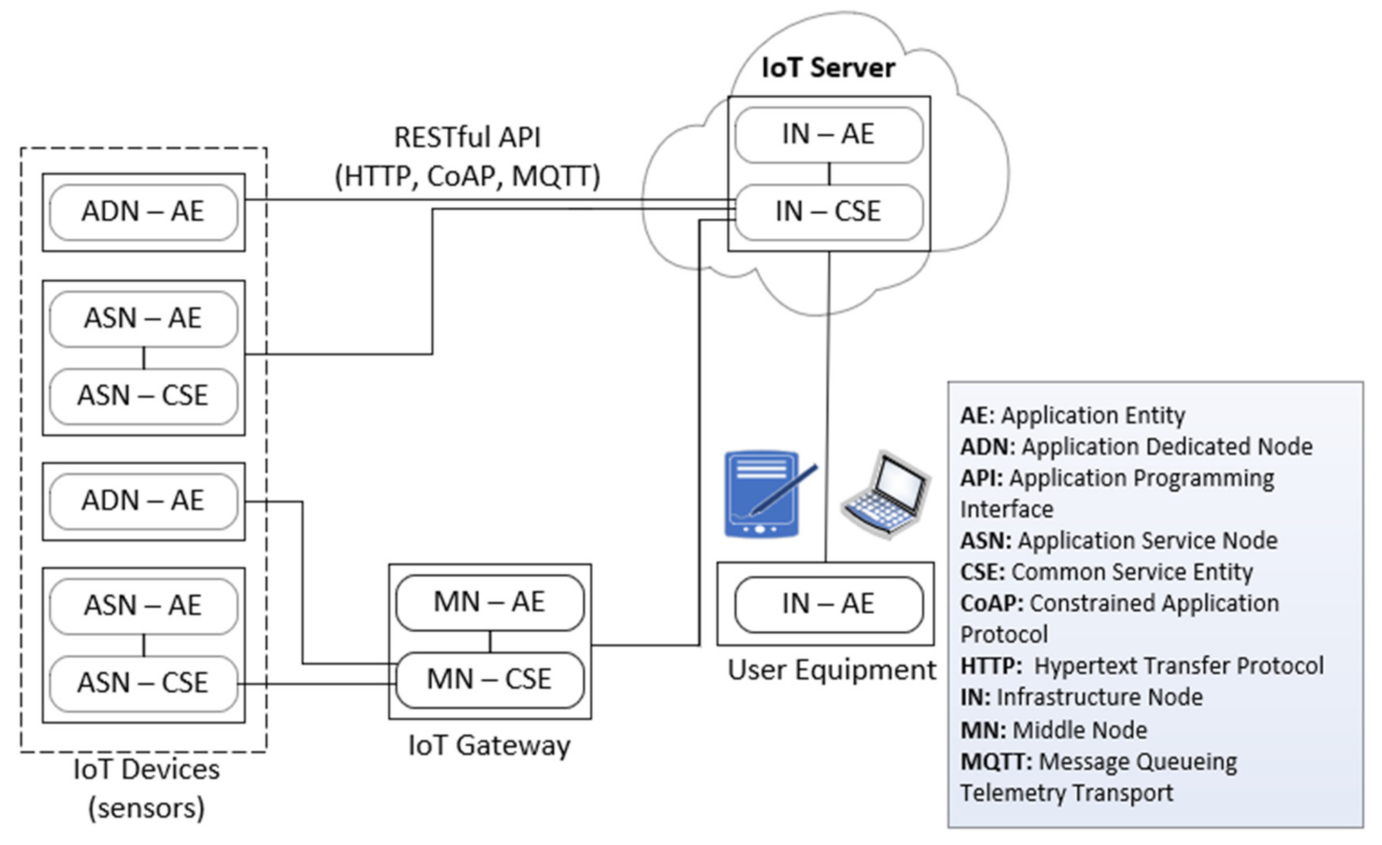
The following is a breakdown of the paper’s structure. The overview of the system is provided in Section 2, while the experimental setup for PM prediction is highlighted in Section 3. The results of the experiment are evaluated and elaborated in Section 4. Finally, in Section 5, the paper is concluded, and ideas for further research are discussed.

2. System Overview

To establish reliability and validity datasets, the authors collected the sensor data via oneM2M standard technology. This method needs a communication interface to support the cyber-physical system (CPS).

2.1. Communication Interface

In this paper, the authors used the RS485 Modbus RTU protocol for communication interface using RJ-116p4c cable. RS485 to USB converter was used to convert data from the sensor using RS485 Modbus RTU protocol to USB for the computer to read and process the data from the sensor. The RS485 protocol data rate can reach 35 Mbit/s over a 10 m connection and 100 Kbit/s over a 1200 m line [14]. The RS485 Modbus RTU protocol has a number of benefits, including reliable communication, interoperability across devices from different manufacturers, and ease of installation and configuration, making it ideal for edge computing [15].

The general architecture used in this study contained hardware, an IoT platform, and an artificial intelligence (AI) platform, as shown in Figure 1. The industrial-grade sensor collected temperature, humidity, PM0.3, PM0.5, PM1, PM2.5, PM5, and PM10 during a three-day period from 24 September to 26 September 2021. The Mobius, an open IoT platform, acts as the gateway, server, and database. This open IoT platform works on an oneM2M technology standard, which is elaborated in the next section.

Jupyter Notebook, based on python programming, was used as the AI platform. The Jupyter Notebook contains a set of open standards for collaborative computing. These open standards can be used by third-party developers to construct bespoke applications with embedded interactive computing based on HTML and CSS on cloud computing. Jupyter Notebook spans through visualization, multimedia, and more with its modular design. In addition to running the code, it saves the code and output as well as markdown notes in an editable document called a notebook. When users save a page in their browser, it is transferred to their notebook server, which saves it as a JSON file with the a.ipynb extension on the disk [16].

2.2. oneM2M Technology Standard

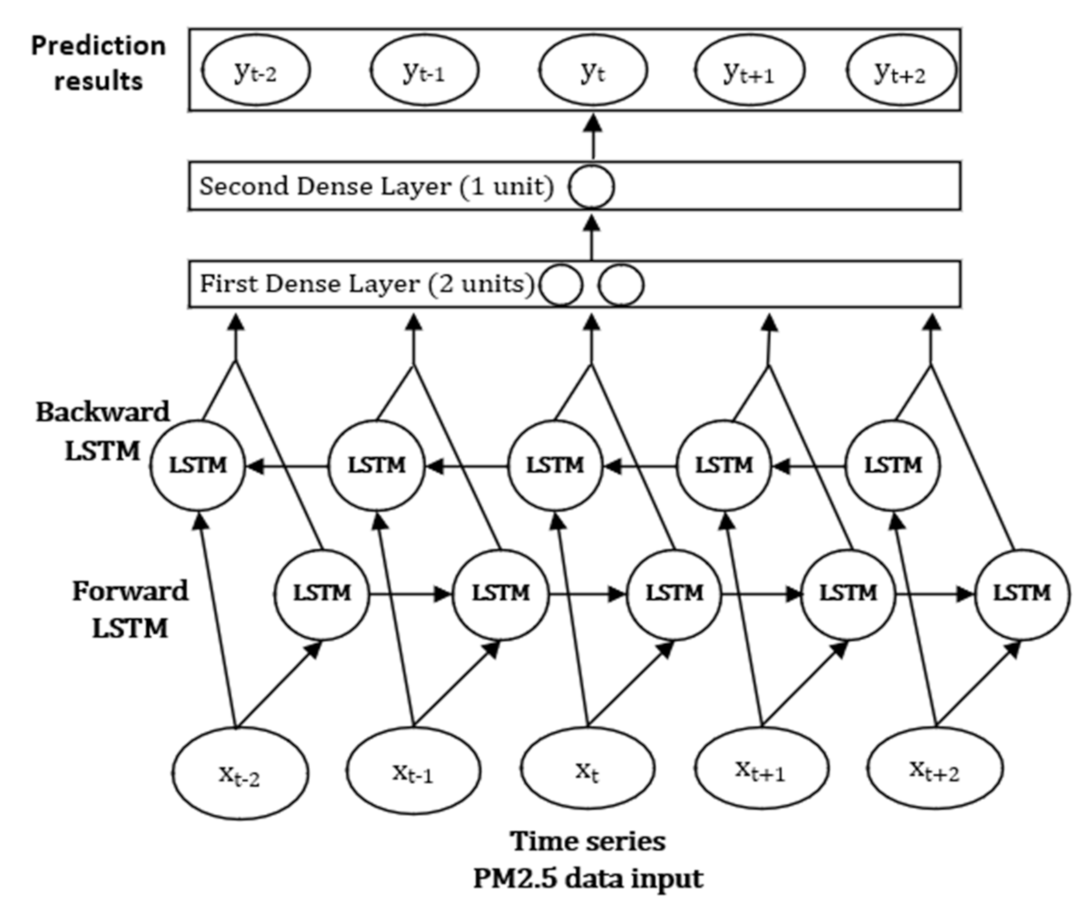
Connected devices have been around for a long time, but they took off after the phrase “Internet of Things” (IoT) was established. As IoT devices began to proliferate, a standard was needed to satisfy new IoT requirements without rewriting pieces that previously had tried and verified specifications. The oneM2M-based platform was built with these concepts in mind to facilitate IoT device and application interoperability and economies of scale. Furthermore, oneM2M’s standard interoperability testing activities are important aspects of a robust standard [17].

The oneM2M standards support IoT applications to discover and interact with any IoT devices. IoT solutions can currently communicate across various silos. This is perfect for distributed and collaborative solutions in domains like smart buildings, smart cities, and smart manufacturing. Furthermore, oneM2M standards were created with the goal of reducing fragmentation, increasing reusability, and lowering costs through scalability [18]. The oneM2M initiative has been working on IoT standards to address fragmentation in the IoT landscape. It focuses on service layer interoperability rather than protocol stacks within the network or internet layers, and hence provides optimal technical standards for building a common horizontal IoT service platform across several domain sectors [19].

The authors used IoT based on oneM2M platforms in the cleanroom of a semiconductor smart factory environment to obtain reliability, validity, and interoperability of data [20]. We can have a common service capability layer in terms of the end-to-end platform with this technology.

In the oneM2M standard, message queuing telemetry transport (MQTT) plays a vital role in collecting and sending sensor data. MQTT is a lightweight application layer protocol for IoT devices. MQTT is a “publish” and “subscribe” protocol in which the sender can deliver information to clients via an intermediary server known as a broker. Each published message has a single topic that clients used to subscribe to a broker. The sole broker defined in the MQTT protocol standard acts as the single point of failure (PoF). Numerous brokers are introduced into a system to increase availability. The IoT platform containing MQTT broker is depicted in Figure 2.

In addition, M2M technology facilitates work by enabling real-time replies on complicated provider networks, such as those found in factories. Real-time control and command with crucial technologies add functions and advantages to supply chain optimization and automation. As a result, use cases should be evaluated via the standard oneM2M technology with real-time command and control [21]. Furthermore, this technology must be incorporated into the current protocol standards. Additionally, oneM2M complies with the international M2M and IoT standards with the goal of creating a single M2M service layer, as shown in Figure 3. It would enable the integration of a wide range of hardware, software, and countless devices from around the world into a system combining M2M-related fields of business into a serviceable system, including telematics, smart transportation, health care, utilities, industrial automation, and smart home applications.

The oneM2M model is a decentralized design that is relatively easy to modify, as shown in Figure 3. Connecting nodes with diverse capabilities construct it. The device component of the IoT or any logical hardware and software service might be defined as an application entity (AE) in this architecture.

The oneM2M service core, the IoT gateway, and the AE application service are all managed by the infrastructure node (IN). It is typically set up on a cloud system platform or server. The IN is the in-charge of the middle layer region with several middle nodes (MNs) that serve IoT service layers and AE application services. In most cases, MNs are created in the IoT gateway. Application service nodes (ASNs) are lightweight common service layers and AE application services are utilized in a remote M2M-based IoT system. In a tiny or limited IoT device system, application dedicated nodes (ADNs) are used to offer sensor monitoring and information return [22].

For visualization of data collected from the sensor, the authors used an oneM2M browser application. This application represents how data sensors (temperature, humidity, PM0.3, PM0.5, PM1, PM2.5, PM5, and PM10) are stored in the MySQL database. As we can see in Figure 4, the green blocks titled cin represent updated sensor data received every second.

3. Methodology

3.1. Multi-Dense Layer BiLSTM

The BiLSTM is a variant of the general LSTM [23]. By processing the incoming data sequences from two directions with two independent LSTMs, we utilized the advantages of both prior and future contexts. The LSTM takes a variable-length sequence x = x₁, x₂, …, x_n as its general input, where $x_i\in {ℝ}^d$and d denotes the features in each time index i. The LSTM preserves its internal hidden state h in each time index, resulting in a hidden sequence of h₁, h₂, …, h_n. At time index t, the hidden vector h_t is modified as follows:

$$i_t=\sigma \left(W_{xi }{x}_t+W_{hi}{h}_{t-1}+b_i\right)$$

(1)

$$c_t=f_t \otimes c_{t-1}+i_t \otimes \tanh \left(W_{xc}{x}_t+W_{hc}{h}_{t-1}+b_f\right)$$

(2)

$$f_t=\sigma \left(W_{xf}{x}_t+W_{hf}{h}_{t-1}+b_f\right)$$

(3)

$$o_t=\sigma \left(W_o{x}_t+W_{ho}{h}_{t-1}+b_o\right)$$

(4)

$$h_t=o_t \otimes \tanh (c_t)$$

(5)

where c, σ, and ⊗ express the cell vector, the sigmoid function, and the element-wise multiplication; i, f, and o indicate to the input, forget, and output gates, respectively.

Figure 5 depicts the proposed Multi-Dense Layer BiLSTM model for predicting PM2.5 concentrations. The algorithm took the PM2.5 concentrations data from the raw data, which contain temperature, humidity, PM0.3, PM0.5, PM1, PM5, and PM10 concentrations. Later, their values are standardized into a range of 0 to 1. The processed dataset is sent into the model for training, and the learned model is then utilized to forecast PM2.5 levels.

The BiLSTM layer is made up of two LSTM layers: a forward layer and a backward layer. The input is recognized by the forward layer $l_t^f$ as ascending range, i.e., t = 1, 2, 3, …, T. Backward layer $l_t^b$, on the other hand, considers the input in descending order, i.e., t = T …, 3, 2, 1. As a result, $l_t^f$ and $l_t^b$ can be combined to generate the output $y_t$. Because they use the same backpropagation through time (BPTT) training mechanism as LSTM networks, BiLSTMs are computationally inexpensive [24].

The backward LSTM layer output sequence $l_t^b$ is calculated using reversed inputs from time t − 2 to t − n, the same as the forward LSTM layer output sequence $l_t^f$. These output sequences are then passed into the function, which combines them into a $y_{t }$output vector. The final output of a BiLSTM layer can be represented as a vector, $Y_t$ = [$y_{t-n }$,…, $y_{t+2}$], where the last element, $y_{t+2}$, is the estimated PM2.5 concentration for the following iteration, similar to the LSTM layer [25].

All the constructed LSTM networks in this study make use of the bidirectional feature. The mathematical equations constituting the BiLSTM model are as follows:

$$l_t^f=\tan \mathrm{h}\left(W_{xl}^f{x}_t+W_{ll}^f{l}_{t-1 }^f+l_{h }^f\right)$$

(6)

$$l_t^b=\tan \mathrm{h}\left(W_{xl}^b{x}_t+W_{ll}^b{l}_{t+1 }^b+l_{h }^b\right)$$

(7)

$$y_t=(W_{ly}^f{l}_t^f+W_{ly}^b{l}_t^b+b_y)$$

(8)

After the BiLSTM layer has processed the data, it is sent to a multi-dense layer with a linear activation function to give continuous value predictions. The dense layer is an utterly interconnected layer, i.e., all neurons in one layer are connected to those in the following [26].

There are two dense layers used in this proposed architecture. In a neural network, a dense layer is one that is tightly coupled to the layer before it. That is, every neuron in the layer before it is coupled to every neuron in the layer before it. This is the most often used layer in artificial neural network networks [27]. The authors used two units in the first dense layer and one unit in the second dense layer. All units in the dense layers contain the sigmoid activation function. In this study, adding more layers to the dense section expectedly can increase the network’s robustness [28].

3.2. Sigmoid Activation Function

The sigmoid is a non-linear activation function frequently employed in feedforward neural networks. It is a bounded differentiable actual function with positive derivatives everywhere and a certain amount of smoothness, defined for real input values. The relationship determines the sigmoid function:

$$f\left(x\right)=\left(\frac{1}{\left(1+ex{p}^{-x}\right)}\right)$$

(9)

The sigmoid function is found in the output layers of deep learning (DL) architectures, and it is used to predict probability-based outputs. It has been successfully employed in binary classification challenges, modeling logistic regression tasks, and other neural network fields. The key advantages of sigmoid functions are that they are simple to learn and that they are commonly utilized in external networks [29].

The sigmoid activation function was elected for this paper since it is ideally suited to tasks that need a continuous-valued output, such as PM2.5 concentration [30].

4. Experimental Setup

The proposed Multi-Dense Layer BiLSTM model is utilized to predict PM2.5 concentrations that can be implemented in the cleanroom of the semiconductor factory. The Tensorflow Keras library was used to implement the proposed system design.

4.1. Dataset and Preprocessing

The collection contains 259,200 data points from 24 September to 26 September 2021. Temperature, humidity, PM0.3, PM0.5, PM1, PM2.5, PM5, and PM10 are among the eight variables listed in

Table 1. Variables consisted in the dataset.

Categories	Input Variables	Unit
Temperature	TEMP	°C
Humidity	HUMID	%RH
Air pollutant variables	PM0.3	µg/m3
Air pollutant variables	PM0.5	µg/m3
Air pollutant variables	PM1	µg/m3
Air pollutant variables	PM2.5	µg/m3
Air pollutant variables	PM5	µg/m3
Air pollutant variables	PM10	µg/m3

. In this experiment, the algorithm contains linear interpolation, which is employed to fill the data if there are any missing values. Linear interpolation produces the best results for all percentages of missing values if compared to other methods, such as the mean method [31]. The authors found no missing data from raw data, which indicates that this is the advantage of the oneM2M system to gather the data [32]. We utilize Equation (9) to normalize the data before inputting it into the proposed method [33]:

$${\overline{x}}_{normalized}=\frac{x-x_{min }}{x_{max-}{x}_{min }}$$

(10)

where $x_{min }$ denotes minimum data, $x_{max }$ is minimum data, and x is the original data. It is critical to create supervised time series data. The input matrices and output matrices are shown below in their many configurations.

For 1 h ahead prediction:

$$\mathrm{Input} \mathrm{matrix}=\left[\begin{array}{ccccc}{x}_{n\left(t=0\right)}& x_{n\left(t=1\right)}& x_{n\left(t=2\right)}& \dots & x_{n\left(t=119\right)}\\ x_{n\left(t=1\right)}& x_{n\left(t=2\right)}& x_{n\left(t=3\right)}& \dots & x_{n\left(t=120\right)}\\ \dots & \dots & \dots & \dots & \dots \\ x_{n\left(t=T-119\right)}& x_{n\left(t=T-118\right)}& x_{n\left(t=T-117\right)}& \dots & x_{n\left(t=T\right)}\end{array}\right]$$

$$\mathrm{Output} \mathrm{matrix}=\left[\begin{array}{ccccc}{x}_{n\left(t=120\right)}& x_{n\left(t=121\right)}& x_{n\left(t=122\right)}& \dots & x_{n\left(t=179\right)}\\ x_{n\left(t=121\right)}& x_{n\left(t=122\right)}& x_{n\left(t=123\right)}& \dots & x_{n\left(t=180\right)}\\ \dots & \dots & \dots & \dots & \dots \\ x_{n\left(t=T+1\right)}& x_{n\left(t=T+2\right)}& x_{n\left(t=T+3\right)}& \dots & x_{n\left(t+60\right)}\end{array}\right]$$

For 2 h ahead prediction:

$$\mathrm{Input} \mathrm{matrix}=\left[\begin{array}{ccccc}{x}_{n\left(t=0\right)}& x_{n\left(t=1\right)}& x_{n\left(t=2\right)}& \dots & x_{n\left(t=239\right)}\\ x_{n\left(t=1\right)}& x_{n\left(t=2\right)}& x_{n\left(t=3\right)}& \dots & x_{n\left(t=240\right)}\\ \dots & \dots & \dots & \dots & \dots \\ x_{n\left(t=T-239\right)}& x_{n\left(t=T-238\right)}& x_{n\left(t=T-237\right)}& \dots & x_{n\left(t=T\right)}\end{array}\right]$$

$$\mathrm{Output} \mathrm{matrix}=\left[\begin{array}{ccccc}{x}_{n\left(t=240\right)}& x_{n\left(t=241\right)}& x_{n\left(t=242\right)}& \dots & x_{n\left(t=359\right)}\\ x_{n\left(t=241\right)}& x_{n\left(t=242\right)}& x_{n\left(t=243\right)}& \dots & x_{n\left(t=360\right)}\\ \dots & \dots & \dots & \dots & \dots \\ x_{n\left(t=T+1\right)}& x_{n\left(t=T+2\right)}& x_{n\left(t=T+3\right)}& \dots & x_{n\left(t=T+120\right)}\end{array}\right]$$

For 3 h ahead prediction:

$$\mathrm{Input} \mathrm{matrix}=\left[\begin{array}{ccccc}{x}_{n\left(t=0\right)}& x_{n\left(t=1\right)}& x_{n\left(t=2\right)}& \dots & x_{n\left(t=479\right)}\\ x_{n\left(t=1\right)}& x_{n\left(t=2\right)}& x_{n\left(t=3\right)}& \dots & x_{n\left(t=480\right)}\\ \dots & \dots & \dots & \dots & \dots \\ x_{n\left(t=T-479\right)}& x_{n\left(t=T-478\right)}& x_{n\left(t=T-477\right)}& \dots & x_{n\left(t=T\right)}\end{array}\right]$$

$$\mathrm{Output} \mathrm{matrix}=\left[\begin{array}{ccccc}{x}_{n\left(t=480\right)}& x_{n\left(t=481\right)}& x_{n\left(t=482\right)}& \dots & x_{n\left(t=839\right)}\\ x_{n\left(t=481\right)}& x_{n\left(t=482\right)}& x_{n\left(t=483\right)}& \dots & x_{n\left(t=840\right)}\\ \dots & \dots & \dots & \dots & \dots \\ x_{n\left(t=T+1\right)}& x_{n\left(t=T+2\right)}& x_{n\left(t=T+3\right)}& \dots & x_{n\left(t+360\right)}\end{array}\right]$$

4.2. Hyperparameters Setting

In this study, the authors evaluated the sequence learning models for short and long-term predictions; experiments were conducted for different time scales, such as one hour, two hours, and three hours ahead.

Table 2. The list of hyperparameters values for the Multi-Dense Layer BiLSTM Method.

Hyperparameter	RNN	LSTM	CNN-LSTM	Single-Dense Layer BiLSTM	Multi-Dense Layer BiLSTM
Model nodes	2 RNN nodes	64 LSTM nodes	128 LSTM nodes	64 BiLSTM nodes	64 BiLSTM nodes
Epoch	20/35/50	20/35/50	20/35/50	20/35/50	20/35/50
Batch size	16	64	16	16	16
Interpolate method	linear	linear	N/A	linear	linear
Train data (% dataset)	64	64%	64%	80%	80%
Validation data (% dataset)	16%	16%	16%	N/A	N/A
Test data (% dataset)	20%	20%	20%	20%	20%
Optimizer	ADAM	SGD	ADAM	ADAM	ADAM
Activation	Linear	Linear	ReLU	Linear	Sigmoid
Learning rate	0.01	0.01	0.001	0.001	0.001
Dense layer	N/A	N/A	3	1	2

elaborates the hyperparameter setting for our proposed model, Multi-Dense Layer BiLSTM. The model’s hyperparameters were determined to achieve the best results. To ensure the consistency of the results, the authors use three kinds of epoch values, 20, 35, and 50. The choice of 80% for training data and 20% for testing data is because this is empirically the best partition into the training and the testing sets [34].

4.3. Performance Criteria

We have predicted PM2.5 concentrations for the three-day dataset; the experiments used three parameters to assess the efficacy of the proposed model: mean square error (MSE) (8), mean absolute error (MAE) (9), and mean absolute percentage error (MAPE) (10) as metrics to appraise the achievement of the Multi-Dense Layer BiLSTM model:

$$\mathrm{MSE}=\frac{1}{n} {\displaystyle {\sum }_{i=1}^n}{\left(y_{i-}{\widehat{y}}_i\right)}^2.$$

(11)

$$\mathrm{MAE}=\frac{1}{n} {\displaystyle {\sum }_{i=1}^n}\left|y_{i-}{\widehat{y}}_i\right|$$

(12)

$$\mathrm{MAPE}=\frac{1}{n} {\displaystyle {\sum }_{i=1}^n}\left|\frac{y_{i-}{\widehat{y}}_i}{y_i}\right|$$

(13)

where $y_{i }$refers to the real value and ${\widehat{y}}_i$refers to the forecasted value, and n expresses the sample size. Higher forecasting accuracy is associated with lower MSE, MAE, and MAPE values [35].

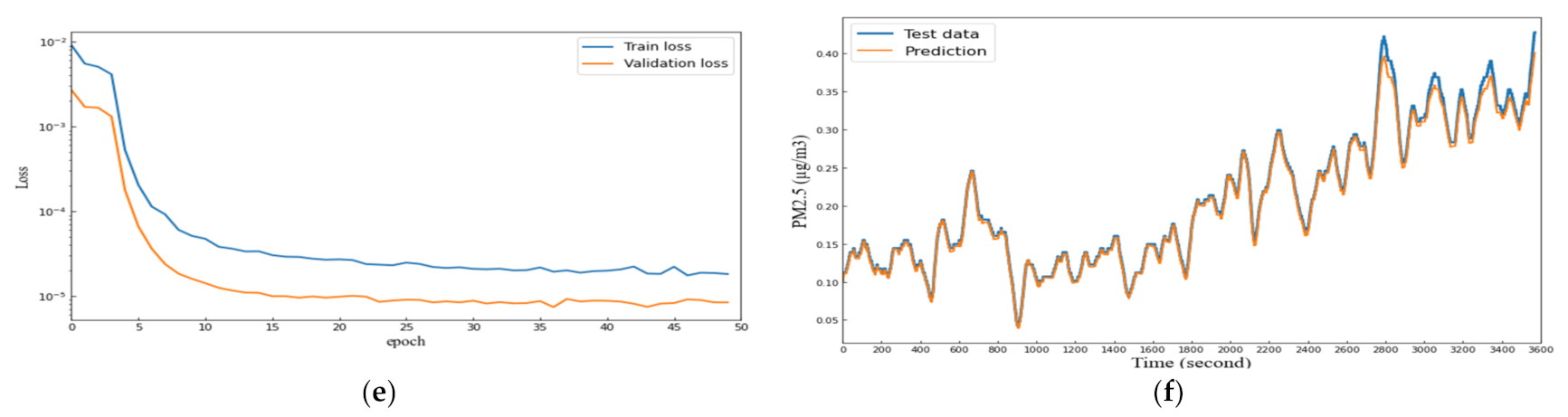
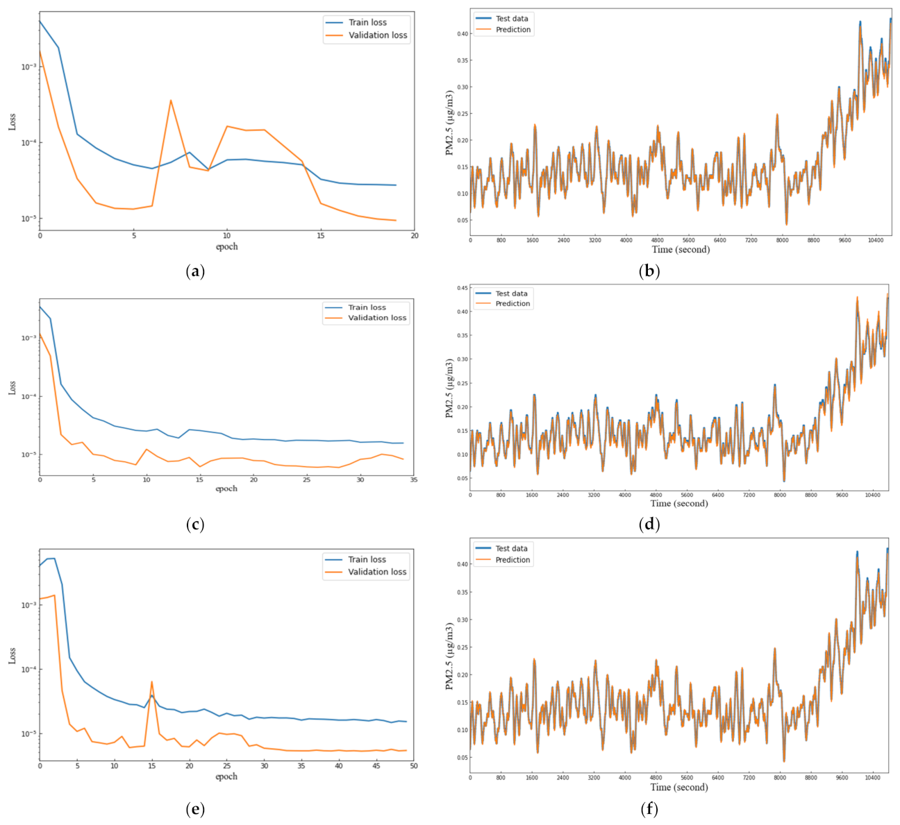
5. Result and Discussion

The proposed Multi-Dense Layer BiLSTM model was used to predict PM2.5 concentrations one hour, two hours, and three hours ahead of the three-day observation, totaling 259,200 s. To test the validity of predictions and support preventive maintenance over a longer timeframe, we set the time forecast into hourly, 2 h, and 3 h.

The proposed Multi-Dense Layer BiLSTM retains low MSE, MAE, and MAPE levels at varied sampling rates, meaning that forecasting accuracy may be assured.

Table 3. The best results from all compared models for PM2.5 prediction with 20, 35, and 50 epochs.

Model	Prediction Time Length	MSE			MAE			MAPE
		20 Epoch	35 Epoch	50 Epoch	20 Epoch	35 Epoch	50 Epoch	20 Epoch	35 Epoch	50 Epoch
RNN	1 h	0.1072	0.1141	0.1001	0.2415	0.2371	0.2199	29.8106	31.0264	27.7334
	2 h	0.1012	0.1138	0.1165	0.1778	0.1986	0.2097	23.89	27.4217	29.8114
	3 h	0.0833	0.0908	0.072	0.2501	0.2337	0.2132	54.1121	56.2735	52.1554
LSTM	1 h	0.0058	0.0048	0.0045	0.0626	0.0548	0.055	11.4597	8.8899	9.1937
	2 h	0.0187	0.0771	0.0217	0.125	0.1985	0.1325	25.617	68.8899	27.6512
	3 h	0.0619	0.0724	0.066	0.1703	0.2023	0.1765	60.5662	67.6347	63.2913
CNN-LSTM	1 h	5.838	3.907	3.69	2.305	1.706	1.676	6.061	3.613	4.332
	2 h	3.871	3.992	3.871	1.659	1.739	1.659	4.864	4.948	4.864
	3 h	8.434	8.434	8.434	2.598	2.598	2.598	7.64	7.64	7.64
Single-Dense Layer BiLSTM	1 h	0.0016	0.0017	0.0016	0.0029	0.0034	0.3266	0.3385	0.3434	0.3047
	2 h	0.0015	0.0027	0.0014	0.318	0.0042	0.3105	0.3046	0.4193	0.2814
	3 h	0.0053	0.0047	0.0063	0.0067	0.0064	0.0073	0.673	0.6433	0.7322
Multi-Dense Layer BiLSTM	1 h	0.0009	0.0014	0.0011	0.0023	0.0028	0.0027	0.2258	0.2849	0.2701
	2 h	0.0014	0.0008	0.0009	0.0027	0.002	0.0021	0.2713	0.1991	0.2058
	3 h	0.001	0.0018	0.0006	0.0022	0.0035	0.0019	0.223	0.3507	0.1873

shows that when the number of epochs in the RNN, LSTM, CNN-LSTM, and Single-Dense Layer BiLSTM algorithms increased, so did the MSE, MAE, and MAPE values, indicating that the three approaches were overfitting. The MSE, MAE, and MAPE values of our approach model, on the other hand, dropped as the prediction time length was increased. These findings acknowledge that, compared to other models, our proposed model predicts PM2.5 concentrations 1 h, 2 h, and 3 h ahead of time and has reached the most preciseness.

Figure 6a–f display the results of predicting PM2.5 concentration one hour ahead, using the Multi-Dense Layer BiLSTM algorithm. From three kinds of epochs experiments, the optimum result between train and validation loss is revealed before the 10th epoch. The blue line in Figure 6a,c,f with the log scale indicates train loss. In contrast, the orange line reflecting validation loss is shown to have the same trend, resulting in the proposed model having the lowest MSE, MAE, and MAPE in 1 h ahead prediction, as mentioned in Table 3. From Figure 6b,d,f, the test data, and prediction data are united very closely. These outputs demonstrate that the proposed model has the best fit to predict PM2.5 concentrations. Compared to the other four models, the results of prediction by the proposed model were the closest to the actual value.

The loss function patterns of the proposed model to estimate PM2.5 concentration for the following two hours are shown in Appendix A, Figure A1a–f. Especially in Figure A1e, the blue and orange lines were closer in epoch 7th, then separated wider until epoch 50th, with relatively having the same trend between these two lines. The test data and prediction data have practically merged in Figure A1b,d,f. These findings suggest that the proposed model is the most accurate in predicting PM2.5 concentrations for 2 h ahead, as mentioned in Table 3.

Similar to the previous experiments one h ahead and two hours ahead, Figure A2a–f depicts the fitting patterns of three hours ahead prediction by the proposed model has attained the best fit. All models were run for 20, 35, and 50 epochs; then, our proposed model, in which the results of prediction are represented by the orange line, came closest to the actual value, which is represented by the blue line. Notably, in Figure A2e, the line of validation loss got a spike in epoch 15th, then it continued to have the same trend with train loss until epoch 50th.

When the number of epochs is increased from 20 to 35, and then 50 epochs, the MSE, MAE, and MAPE values from the proposed model tend to decrease to the lowest error compared to other methods. These results demonstrate that Multi-Dense Layer BiLSTM has the best fit pattern than the other four models. The authors took a sample to combine the fitting trends from all models for one hour ahead prediction, with each model run by 20 epochs, which are shown in Figure 7.

In the zoomed Figure 7, the authors took sample lines from all compared models from 25 to 35 s, indicating that the proposed model represented by the orange line has the closest distance to the real data represented by the blue line. The proposed model and single-dense layer BiLSTM represented by the green line have a close connection. This result shows that the proposed model, which uses multi-dense layers, could empower network stability [28].

From Figure 7, we can also see that the CNN-LSTM model, represented by the red line, has the furthest distance from the real data. This result is suitable to the values mentioned in Table 3. This is understandable given that CNN-LSTM is essentially slower due to its operations and necessitates a lengthy process [36].

6. Conclusions

PM2.5 concentrations can have a significant impact on the semiconductor plant product quality. Therefore, a robust framework is required to monitor, analyze, and predict air quality with additional visualization services. It is imperative to develop an accurate prediction method to ensure awareness regarding the prospective air quality in the clean rooms among the personnel working at semiconductor manufacturing sites.

In this study, we built PM monitoring infrastructure using an industrial-grade sensor to meet the quality and compatibility standards of the industrial sector. In particular, open-source software platforms compliant with oneM2M standard technology were used to provide a standardized approach to access the obtained PM datasets, allowing us to construct globally applicable and access-independent PM apps using oneM2M-defined REST APIs.

Furthermore, for one hour, two hours, and three hours forecasts, the proposed technique, Multi-Dense Layer BiLSTM, was shown to have the lowest errors in terms of MSE, MAE, and MAPE as compared to the RNN, LSTM, CNN-LSTM, and Single-Dense Layer BiLSTM models. The findings can also be used by policymakers in semiconductor factories to control the air quality of the cleanroom using HVAC based on this proposed model of PM2.5 prediction.

Despite the excellent results, there are a few difficulties that we would like to address in future work, such as the large memory and computing time required by our model in the case of big datasets.

To further improve the prediction, cumulative airborne characteristics of the cleanroom must be analyzed. Further steps include constructing integrated predictive, preventive, and prescriptive maintenance based on the PM prediction with suitable control function services in cleanroom semiconductor manufacturing.

References

1. Park, S.H.; Kim, S.; Baek, J.G. Kernel-Density-Based Particle Defect Management for Semiconductor Manufacturing Facilities. Appl. Sci. 2018, 8, 224. [Google Scholar] [CrossRef] [Green Version]
2. Choi, K.-M. Airborne PM2.5 Characteristics in Semiconductor Manufacturing Facilities. AIMS Environ. Sci. 2018, 5, 216–228. [Google Scholar] [CrossRef]
3. Prihatno, A.T.; Nurcahyanto, H.; Ahmed, M.F.; Rahman, M.H.; Alam, M.M.; Jang, Y.M. Forecasting PM2.5 Concentration Using a Single-Dense Layer Bilstm Method. Electronics 2021, 10, 1808. [Google Scholar] [CrossRef]
4. Wali, F.; Knotter, D.M.; Kuper, F.G. Impact OfNano Particles on Semiconductor Manufacturing. In Proceedings of the 2008 IEEE International Conference on Multi Topi, Karachi, Pakistan, 23–24 December 2008; pp. 97–99. [Google Scholar]
5. The International Technology Roadmap for Semiconductors 2.0. Available online: https://www.semiconductors.org/wp-content/uploads/2018/06/4_2015-ITRS-2.0-ESH.pdf (accessed on 30 December 2021).
6. Chang-Hoi, H.; Park, I.; Oh, H.R.; Gim, H.J.; Hur, S.K.; Kim, J.; Choi, D.R. Development of a PM2.5 Prediction Model Using a Recurrent Neural Network Algorithm for the Seoul Metropolitan Area, Republic of Korea. Atmos. Environ. 2021, 245, 118021. [Google Scholar] [CrossRef]
7. Tsai, Y.T.; Zeng, Y.R.; Chang, Y.S. Air Pollution Forecasting using RNN with LSTM. In Proceedings of the 2018 IEEE 16th International Conference on Dependable, Autonomic and Secure Computing, 16th International Conference on Pervasive Intelligence and Computing, 4th International Conference on Big Data Intelligence and Computing and Cyber Science and Technology Congress (DASC/PiCom/DataCom/CyberSciTech), Athens, Greece, 12–15 August 2018; pp. 1068–1073. [Google Scholar]
8. Park, J.; Chang, S. A Particulate Matter Concentration Prediction Model Based on Long Short-Term Memory and an Artificial Neural Network. Int. J. Environ. Res. Public Health 2021, 18, 6801. [Google Scholar] [CrossRef]
9. Huang, C.J.; Kuo, P.H. A Deep Cnn-Lstm Model for Particulate Matter (Pm2.5) Forecasting in Smart Cities. Sensors 2018, 18, 2220. [Google Scholar] [CrossRef] [Green Version]
10. Li, T.; Hua, M.; Wu, X.U. A Hybrid CNN-LSTM Model for Forecasting Particulate Matter (PM2.5). IEEE Access 2020, 26933–26940. [Google Scholar] [CrossRef]
11. Seong, N. Deep Spatiotemporal Attention Network for Fine Particle Matter 2.5 Concentration Prediction with Causality Analysis. IEEE Access 2021, 9, 73230–73239. [Google Scholar] [CrossRef]
12. Castelli, M.; Clemente, F.M.; Popovič, A.; Silva, S.; Vanneschi, L. A Machine Learning Approach to Predict Air Quality in California. Complexity 2020, 2020, 8049504. [Google Scholar] [CrossRef]
13. Zhang, B.; Zhang, H.; Zhao, G.; Lian, J. Constructing a PM2.5 Concentration Prediction Model by Combining Auto-Encoder with Bi-LSTM Neural Networks. Environ. Model. Softw. 2020, 124, 104600. [Google Scholar] [CrossRef]
14. Wu, J.; Tian, K.; Dong, Q.; Sun, L.; Zhang, L.; Liu, X. A Low Voltage Low Power Adaptive Transceiver for Twisted-Pair Cable Communication. IEEE Trans. Nucl. Sci. 2015, 62, 3140–3147. [Google Scholar] [CrossRef]
15. Seneca. The Advantages of ModBUS RTU Protocol. Available online: https://blog.seneca.it/en/the-advantages-of-modbus-rtu-protocol/ (accessed on 30 December 2021).
16. Prihatno, A.T. Artificial Intelligence Platform Based for Smart Factory. In Proceedings of the Korea Artificial Intelligence Conference, online, South Korea, 16–18 December 2020; pp. 1–2. [Google Scholar]
17. Figueredo, K. Building a Flexible Standard to Deliver a Thriving IoT Ecosystem. IEEE Commun. Stand. Mag. 2020, 4, 10–11. [Google Scholar]
18. oneM2M. Partners Benefits of oneM2M. Available online: https://www.onem2m.org/using-onem2m/what-is-onem2m (accessed on 12 November 2021).
19. Yun, J.; Woo, J. IoT-Enabled Particulate Matter Monitoring and Forecasting Method Based on Cluster Analysis. IEEE Internet Things J. 2021, 8, 7380–7393. [Google Scholar] [CrossRef]
20. Prihatno, A.T.; Nurcahyanto, H.; Jang, Y.M. Smart Factory Based on IoT Platform. In Proceedings of the KIC Summer Conference, online, Belgium, 22–23 October 2020; pp. 2–4. [Google Scholar]
21. Zhao, R.; Wang, L.; Zhang, X.; Zhang, Y.; Wang, L.; Peng, H. A oneM2M-Compliant Stacked Middleware Promoting IoT Research and Development. IEEE Access 2018, 6, 63546–63559. [Google Scholar] [CrossRef]
22. Xu, S.S.D.; Chen, C.H.; Chang, T.C. Design of oneM2M-Based Fog Computing Architecture. IEEE Internet Things J. 2019, 6, 9464–9474. [Google Scholar] [CrossRef]
23. Shabanian, S.; Arpit, D.; Trischler, A.; Bengio, Y. Variational Bi-LSTMs. arXiv 2017, arXiv:1711.05717. [Google Scholar]
24. Shah, S.R.B.; Chadha, G.S.; Schwung, A.; Ding, S.X. A Sequence-to-Sequence Approach for Remaining Useful Lifetime Estimation Using Attention-Augmented Bidirectional LSTM. Intell. Syst. Appl. 2021, 10–11, 200049. [Google Scholar] [CrossRef]
25. Li, Y.H.; Harfiya, L.N.; Purwandari, K.; Lin, Y. Der Real-Time Cuffless Continuous Blood Pressure Estimation Using Deep Learning Model. Sensors 2020, 20, 5606. [Google Scholar] [CrossRef]
26. Rampurawala, M. Classification with TensorFlow and Dense Neural Networks. Available online: https://heartbeat.fritz.ai/classification-with-tensorflow-and-dense-neural-networks-8299327a818a (accessed on 1 June 2021).
27. Verma, Y. A Complete Understanding of Dense Layers in Neural Networks. Available online: https://analyticsindiamag.com/a-complete-understanding-of-dense-layers-in-neural-networks/] (accessed on 3 December 2021).
28. Islam, M.N.; Sulaiman, N.; Al Farid, F.; Uddin, J.; Alyami, S.A.; Rashid, M.; Majeed, A.P.P.A.; Moni, M.A. Diagnosis of Hearing Deficiency Using EEG Based AEP Signals: CWT and Improved-VGG16 Pipeline. PeerJ Comput. Sci. 2021, 7, e638. [Google Scholar] [CrossRef]
29. Nwankpa, C.; Ijomah, W.; Gachagan, A.; Marshall, S. Activation Functions: Comparison of Trends in Practice and Research for Deep Learning. arXiv 2018, arXiv:1811.03378. [Google Scholar]
30. Narayan, S. The Generalized Sigmoid Activation Function: Competitive Supervised Learning. Inf. Sci. 1997, 99, 69–82. [Google Scholar] [CrossRef]
31. Noor, N.M.; Al Bakri Abdullah, M.M.; Yahaya, A.S.; Ramli, N.A. Comparison of Linear Interpolation Method and Mean Method to Replace the Missing Values in Environmental Data Set. Mater. Sci. Forum 2015, 803, 278–281. [Google Scholar] [CrossRef]
32. Alaya, B.; Medjiah, S.; Monteil, T.; Drira, K.; Khalil, D. Towards Semantic Data Interoper-Ability in oneM2M Standard. IEEE Commun. Mag. Inst. Electr. Electron. Eng. 2015, 53, 35–41. [Google Scholar]
33. Gao, X.; Li, W. A Graph-Based LSTM Model for PM2.5 Forecasting. Atmos. Pollut. Res. 2021, 12, 101150. [Google Scholar] [CrossRef]
34. Gholamy, A.; Kreinovich, V.; Kosheleva, O. Why 70/30 or 80/20 Relation Between Training and Testing Sets: A Pedagogical Explanation. Dep. Tech. Rep. 2018, 2, 1–6. [Google Scholar]
35. Lendave, V. A Guide to Different Evaluation Metrics for Time Series Forecasting Models. Available online: https://analyticsindiamag.com/a-guide-to-different-evaluation-metrics-for-time-series-forecasting-models/ (accessed on 30 December 2021).
36. Bhuiya, S. Disadvantages of CNN Models. Available online: https://iq.opengenus.org/disadvantages-of-cnn/ (accessed on 30 December 2021).
Figure 1. General architecture of this study.
Applsci 12 02260 g001
Figure 2. IoT platform design and architecture with MQTT.
Applsci 12 02260 g002
Figure 3. The oneM2M architecture model.
Applsci 12 02260 g003
Figure 4. Real-time sensor data acquisition visualization using oneM2M browser application.
Applsci 12 02260 g004
Figure 5. Proposed architecture of Multi-Dense Layer BiLSTM model.
Applsci 12 02260 g005
Figure 6. Result of loss function using the proposed model for 1 h ahead prediction (a,b) 20 epochs. (c,d) 35 epochs. (e,f) 50 epochs.
Applsci 12 02260 g006aApplsci 12 02260 g006b
Figure 7. Comparison of all models to predict PM2.5 concentrations for one hour ahead.
Applsci 12 02260 g007