Article

Bootstrap–CURE: A Novel Clustering Approach for Sensor Data—An Application to 3D Printing Industry

Knowledge Engineering and Machine Learning Group at Intelligent Data Science and Artificial Intelligence Research Centre, Universitat Politecnica de Catalunya, 08034 Barcelona, Spain
*
Author to whom correspondence should be addressed.
These authors contributed equally to this work.
Appl. Sci. 2022, 12(4), 2191; https://doi.org/10.3390/app12042191
Submission received: 14 December 2021 / Revised: 13 February 2022 / Accepted: 17 February 2022 / Published: 19 February 2022
(This article belongs to the Special Issue Women in Artificial intelligence (AI))

Abstract

:
The agenda of Industry 4.0 highlights smart manufacturing by making machines smart enough to make data-driven decisions. Large-scale 3D printers, being one of the important pillars in Industry 4.0, are equipped with smart sensors to continuously monitor print processes and make automated decisions. One of the biggest challenges in decision autonomy is to consume data quickly along the process and extract knowledge from the printer, suitable for improving the printing process. This paper presents the innovative unsupervised learning approach, bootstrap–CURE, to decode the sensor patterns and operation modes of 3D printers by analyzing multivariate sensor data. An automatic technique to detect the suitable number of clusters using the dendrogram is developed. The proposed methodology is scalable and significantly reduces computational cost as compared to classical CURE. A distinct combination of the 3D printer’s sensors is found, and its impact on the printing process is also discussed. A real application is presented to illustrate the performance and usefulness of the proposal. In addition, a new state of the art for sensor data analysis is presented.

1. Introduction

Industry 4.0 [1] has been revolutionizing the manufacturing practices with a strong influence on mechanization and automation. Inadvertently, this also brings up the importance of sensors and their pattern analysis. A sensor is a physical device that detects or measures an external signal and records it or responds to it. A comprehensive definition and types of sensors are explained in the work [2]. New generation machines are now equipped with dozens of sensors to extract data at high temporal resolution. An exhaustive analysis of the data provided by sensors can help obtain crucial information about the health of the overall system, as well as developing tools for faster knowledge extraction and automation. Sensor data are typically unlabeled and thus demand an unsupervised methodology to characterize their impact on a machine and also explainable AI techniques to interpret the results from a semantic point of view. When a 3D printer works in the real production environment under smart manufacturing [3], most of its activities are completely automated and governed by an electronic control system. There can still be situations when the printer stops a print job or results in some fault, and this leads to a lot of open questions. A proper understanding of machine operations under various conditions can help answer what factors cause such problems.
The main goal of this paper is to use data to study the behavior of the 3D printer machine to better understand its operation and to obtain insights with respect to the control systems that govern the printing process in a real production environment. Understanding what factors result in a successful or unsuccessful job and how they are expressed through sensor data is crucial for the future development of 3D printer technologies.
It is important to note that this behavioral study is conducted from the perspective of aiding the printer manufacturer in predictive maintenance as well as gaining a superior understanding of the printing subsystems and their operation modes by solely using the multivariate sensor data.
This research addresses the enterprise-grade multi-jet fusion 3D printers working in a real production environment. As these machines operate in the customer’s environment with strict confidentiality agreements, neither confidential data (such as print-layer images or video) nor any external modification to the printer are possible, and this is why this approach is based on the mere use of sensor data. This situation also applies to other domains outside 3D printing, such as wastewater treatment plants [4], gas turbines [5], aero-generators [6], etc. Therefore, the methodology proposed in this paper may be useful in other Industry 4.0 application domains as well.
The long-term goal of this research is to build an intelligent diagnosis system that can understand what leads to a failure while the machine is operating and can react in real time to restore the normal behavior of the machine. In the long term, it is also expected to predict such failures in advance and react preventively. The focus of this paper is a preliminary step to reach these goals. This step consists of identifying and understanding the main operation modes exhibited by the machine and eventually association with different kinds of failures.
Thus, the main goal of the proposal is to provide a tool that identifies states of operation in the 3D printing machine without needing any prior hypotheses on the number of clusters and is also suitable for analyzing a large amount of data in a rather short computation time. This is directly related to the use of hierarchical clustering methods, where the real number of existing clusters is not required as an input parameter. However, hierarchical clustering is of quadratic complexity and does not scale up to large datasets automatically.
Although the research is focused on analyzing sensor data from 3D printers, the clustering methodology itself is agnostic to the domain and can be used in any generic application wherein data from sensors are used. Thus, the final and fourth contribution of this paper is to provide a general conceptualization of the field of sensor data.
The structure of the paper is as follows. First, a summary of the motivation behind the research, including the high-level goals, is presented in Section 1. A brief overview of 3D printing is shared in Section 2, followed by the literature review of state-of-the-art models in Section 3. The contributions of the paper are explicitly mentioned in Section 4. Section 5 describes the methodology and continues to Section 6, providing an application from a real-life dataset from 3D printing. Section 7 discusses the proposed methodology in an industrial setting of 3D printers. The paper finally rests with the conclusion in Section 8 along with the future lines of work in the research.

2. 3D Printing Process

The term, additive manufacturing (commonly known as 3D printing), has been drawing attention from different sections of the industries by allowing the digitization of physical models. In [7], a review of the main 3D printing technologies can be found.
One of the major advantages of 3D printing is the ability to produce a monolithic structure of complex geometry. This is possible by building parts through a stack of thin cross sections in an additive manner. Hence, this type of printing also saves print material, which is often wasted in traditional subtractive manufacturing. Some of the key 3D printing technologies are as follows [8]:
  • Fused deposition modeling: Machine lets the plastic filament melt and extrude through nozzles onto the bed platform, where it is cooled and solidified.
  • Binder jetting: Machine distributes a layer of powder onto a build platform, and a bonding agent helps to fuse the parts. The process keeps repeating until the parts are built up in the powder bed.
  • Laser sintering: Uses a laser as a power source to aim at points in 3D space to sinter the powder material and create a solid part.
  • Laser melting: Machine uses laser(s) to melt metal powder.
  • Stereo-lithography: Machine builds parts out of liquid photopolymer through polymerization activated by a UV laser.
This paper focuses on finding interpretable models to describe the work done on anonymized sample sensor measurements from HP Multi-Jet 3D Fusion printers. According to the overview provided in additive manufacturing [7], the jet-fusion technology is a further improvement developed by HP, on the fused deposition modeling and polyjet technologies. A brief technical introduction of multi-jet fusion technology is provided in the work [9]. Such 3D printers are equipped with dozens of sensors placed across different components to measure and control factors, such as temperature, humidity, velocity, pressure, etc. A 3D printing process is a complex job, where many parameters must align among themselves for the success of the job. A brief technical introduction of multi-jet fusion technology is provided in the work by [9].
The data collected through the sensors network of the printer are produced in a streaming mode and sent to a cloud-based server for further processing. Analyzing the sensor-based network is challenging in the sense that it is required to run the analysis on the fly and be able to ingest large amount of sensor data rather quickly.

3. State-of-the-Art

The literature review is divided into two major parts, focusing, respectively, on data science applications in sensor analysis (Section 3.1) and the methods to scale hierarchical clustering and identify the best number of clusters (Section 3.2.1).

3.1. Data Science Applications in Sensor Analysis

The field of sensor analysis has been quite active in recent years, with both academics and industry contributing to the research alike.
Although one can find innumerable data science applications of sensor data (including the one in 3D printing) in the literature, and it is difficult to write an exhaustive survey, the authors identify the following main research areas.
  • Anomaly detection;
  • Automatic reporting and visualization;
  • Pattern analysis;
  • Process control;
  • Predictive maintenance.
The authors were thus able to synthesize the map displayed in Figure 1. The authors conclude that most of the literature in this field can be grouped into five broad categories as shown in Figure 1. This picture helps to organize the contents of this section.

3.1.1. Anomaly Detection

A majority of works in recent times focus on using sensor data to detect anomalies in real time or offline data. This itself is a fairly general framework with applications in a wide variety of domains, ranging from healthcare, autonomous vehicles, printing, internet-of-things, etc. The literature can further be subdivided based on the kind of algorithms used for the modeling. Deep learning-based methods are most popular in this category [10], sometimes in their classical supervised version [11,12], and sometimes in an unsupervised deep learning approach, such as Ref. [13] applying autoencoders to detect anomalies in an aircraft system, and Parllaku et al. [14] and Karna et al. [15] finding anomalies in 3D printing processes. Although deep learning techniques generally have high accuracy, there is a high variety of architectures depending on each concrete application. This implies that the sensor data behave differently as per the application field. In addition, the inability of neural network models, in general, to explain anomalies is a big industrial challenge for research purposes.
Although relatively fewer, there are still several studies using other machine learning methods, most of them hybrid approaches combining different techniques: Ref. [16], where hybrid random forest with wavelet transform is developed to recognize vehicle steering mode and further detect abnormal behavior; some references based on the combination of support vector machines with other techniques, such as deep belief networks [17] and DBScan [18]; or statistical applications, such as kernel PCA [19]. These works propose a hybrid scheme of using a previously unsupervised method to identify anomalies and build a predictive model on top of using SVM. Although SVM provides more explainable predictions than deep learning, their learning times are not scalable to big-data-based real industrial scenarios yet.

3.1.2. Automatic Reporting and Visualization

Here, the authors find works contributing mainly to visualizing traffic coming from sensors and interpreting their patterns. From analyzing EEG (ElectroEncephaloGram) [20,21], to visualizing traffic data [22], a good visualization tool can allow interacting with anomalies in real time [23] or combine common system abnormalities with simple descriptive statistics [24]. In this field, interactivity and visual interfaces provide business dashboards and tools to track key business process indicators. This field focuses more on the human–computer interaction than intensive algorithmic models.

3.1.3. Pattern Analysis

A typical data challenge in industrial applications is to discover or recognize patterns from sensor data. A large number of works use clustering techniques and related methods to discover patterns or characterize features. In [25], a theoretical approach to density estimation clustering on sensor networks is found. Although the literature is limited with respect to pattern recognition research in Industry 4.0, some important works have been found in the following. In [26], the unsupervised deep convolutional network was used to recognize patterns of cyber attacks in industrial wastewater treatment plants, whereas [27] used Markov models on sensor data to identify patterns of energy consumption and comfort management in intelligent buildings. Some noteworthy work in the characterization of sensor signals using k-means clustering was done by Hromic et al. [28] on sensor data for air quality, and Loane et al. [29] used clustering to find patterns of households based on domestic sensors. Ref. [30] used k-means and support vector machines (SVM) to first identify patterns of print conditions in selective laser melting machines and then identified them with an SVM model.
Some of these works are approaching the dynamics of the system. In [26], a univariate approach of time series modeling was followed, while in [27], a multivariate approach was used for characterizing the relationships among the sensors along time. All other works are based on clustering, finding groups of similar objects under a multivariate approach. K-means is used frequently, although it requires many runs and finding the optimization criteria to identify the right number of clusters. Only one work used hierarchical clustering [29], showing evidence that the optimal number of clusters is obtained by running several k-means and optimizing the silhouette index results in the same number of clusters given by the dendrogram of the hierarchical clustering. Specific to 3D printing, only one work is found that combined k-means with a classifier to identify types of operation with a predictive model. The authors also want to use clustering to identify types of operation of 3D printers and thus understand the relationships among sensors. A detailed overview of the related works in clustering is provided in Section 3.2.

3.1.4. Process Control

Process control and monitoring sensors is highly relevant for Industry 4.0. The literature is relatively limited and mostly comes from the field of time series forecasting or supervised machine learning based on images.
A number of references describe supervised learning applications especially on small-scale 3D printers (commonly based on fused-deposition-modeling principle). Some notable works that help in detecting quality of 3D printed part are presented in [31,32,33,34,35,36]. Although these works provide valuable contributions to 3D printing especially in detecting and monitoring part quality, they assume the possibility of using tagged data to train the models, and they are mainly based on images of video processing. These approaches are out of the scope of this research for several reasons:
  • The need to obtain supervised data every time a model has to be trained is unrealistic in real Industry 4.0 manufacturing.
  • In a customer environment with a fleet of 3D printers installed, obtaining global knowledge of the machines’ health from the manufacturer’s perspective would require analyzing data anonymously, as any confidential data (involving 3D print design or the print images) other than the sensor records cannot be shared or stored outside the customer site.
  • Additionally, some of these works assume the possibility of installing additional cameras into the 3D printers; however, in an industrial setting, this is not always possible, as only customers have the sole decision-making authority to make any changes.
The time series approach based on sensor data seems a more suitable reference for our research. In this regard, some works merit a reference. In [37], an application from the iron and steel industries processes sensor data through a discrete-time extended Kalman filter for both process state estimation and sensor data fusion. Understanding the sensors’ patterns and invoking real-time process control can tremendously improve print job success on a whole. In the context of 3D printing, process control helps monitor the evolution of the part by printing layers and guarantees the overall success of the job. In process control, some works can be found in the field of 3D printing, although they are not suitable for our research goals. In [38], exponential weighted moving average (EWMA) charts are used to monitor the process parameters and detect shifts in the fused deposition printing process and thereby assess geometrical deformations of the printed part. In [39], Zang et al. present a novel scheme of simulating surface properties of printed part by defining in-control and out-of-control specifications and use bootstrap sampling to estimate the control limit of several control charts. Both of these works consider small-scale 3D printers. In the context of a large-scale 3D printer, such as multi-jet fusion, such approaches do not apply, as the machine is far more complex, so process monitoring cannot be limited to just one surface of the part, and external cameras are also not applicable. However, it is interesting to see the idea of introducing bootstrap techniques in the processing to scale up the modeling.

3.1.5. Predictive Maintenance

Predictive maintenance [40,41], is the latest trend in Industry 4.0 to provide superior customer experience by using an automated and highly interconnected network of sensors to predict faults at the early stage and minimize industrial downtime. Predictive maintenance is a wider approach and mostly includes anomaly detection by detecting faults at an early stage in addition to estimating the remaining useful life and time-to-failure of equipment in industrial processes. A general framework of designing predictive maintenance solution is described in [42] with a case study from steel industries to estimate the degradation of coiler drums, using the discrete Bayesian filter. Bonci et al. in [43] used the wavelet decomposition model to analyze and predict faults in Cartesian robots based on the motor current signal, while Lin et al. in [44] presented an ARIMA-based time series prediction approach to predict the remaining useful life of the target device in the factory settings based on aging features. Gibert et al. [45] used clustering techniques to assess the health of the wind turbines based on sensor data and introduced some post-processing techniques to interpret the meaning of the clusters and the associated healthy state they represent.
Deep learning techniques are also frequently used in predictive maintenance. In [46], autoencoders and deep belief networks were proposed for early fault detection in digital manufacturing. In [47], dynamic predictive maintenance framework was proposed for the turbofan engine by using deep learning. In [48], deep learning was used on IoT for predictive maintenance of a Porsche car based on the sound recorded on different parts of the engine.
Shi et al. [49] concluded that multi-core CPU machines do not scale sufficiently well for training deep neural networks and still require a dedicated GPU. This is a a serious limitation for those Industry 4.0 applications with machines embedded with computation-intensive hardware, such as 3D printers, as adding a GPU implies increasing the printing time of jobs. This also adds extra cost to the total value of the machine. Additionally, deep learning models are generally assumed to be black-box in nature and cannot explain the proposed predictions, which is critical in a decision-making context, as predictive maintenance often is.
Thus, there is no existing method known to be effective in analyzing and controlling the manufacturing process in the context of multi-jet large-scale 3D printers [50]. A machine like a multi-jet 3D printer, running non-stop and generating tons of data, would thus require appropriate statistical techniques to ingest data and process them rather rapidly. Hence, for a suitable insertion in real production systems, near-real-time and non-supervised approaches are required; classic deep learning approaches for predictive maintenance might not be suitable.
In this paper, the authors are attempting to establish telemetry monitoring and analysis, using an unsupervised learning approach (hierarchical clustering in particular) with a focus on explainable artificial intelligence methods.

3.2. Clustering Strategies

In general, clustering refers to the task of grouping similar objects. Xu et al. [51] provided a comprehensive survey of various clustering algorithms. While hard-clustering algorithms (e.g., hierarchical and k-means) uniquely assign an object into a single cluster, soft-clustering methods, such as fuzzy-clustering, rather assign each object with a certain membership degree to belong to different clusters. Fuzzy clustering provides a fuzzy partition as a result and requires defuzzification in the post-processing step.
Gupta et al. [52] presented a new approach based on evolutionary multi-objective optimization in fuzzy clustering to identify clusters at different levels of fuzziness. Lahmar et al. [53] provided a self-adaptive fuzzy c-means method to find the number of clusters; however, scalability to large datasets is not guaranteed in the paper. Shirkhorshidi et al. [54] provided an evolving fuzzy-clustering approach, where a small subset of data is clustered in every epoch, centroids are generated, and a global clustering takes place using k-means on these centroids. Although this work also elaborates on the idea of finding previous clusters and making a further clustering over centroids, the use of k-means demands a clear hypothesis on the number of clusters in each epoch, which is not possible in the real 3D printer management application field that the authors are targeting.
Among non-fuzzy clustering algorithms, k-means is one of the most popular for its ability to work on large datasets. Sebastian et al. [55] provided an interesting application of k-means clustering in the characterization of snore signals in the context of upper-airway collapse. Chakraborty et al. [56] proposed the Lass-weighted k-means algorithm specifically useful for a high-dimensional dataset, such as gene-expression data. Another interesting algorithm was developed by Gondeau et al. [57], using object-weighting in k-means clustering. The algorithm therein can help as a data preprocessing step to deal with outliers, especially in the case of noisy data. This method attempts to increase the weights of the outliers instead of removing them from the study. The results of this algorithm on both simulated and real-life datasets are quite promising too. However, the context of the current research is far from the situation where the real number of clusters to be built is known a priori, and all partitioning methods, including k-means, require the number of clusters to be found as an input parameter. For this reason, the authors will not work with partitioning methods.
In some recent works, the use of evolutionary and meta-heuristic optimization is also seen in the context of clustering. Li et al. [58] used gravitational search to optimize the number of clusters (obtained using DBSCAN approach) in multiple iterations. The final number of clusters is, however, decided manually. The approach seems scalable to large datasets; however, the requirement of running the algorithm in multiple iterations limits the application on cases where near-real-time data are to be analyzed rather quickly, such as the data from 3D printers’ sensors. In the current research, the 3D printing sensor data require quicker analysis on a large amount of data, and running multiple iterations may not be acceptable from the practical point of view. Liu et al. [19] proposed another meta-heuristic optimization to improve the maximum-entropy clustering method. The applications of such an algorithm on large-scale data would be interesting to check.
In the current age of deep learning, the graph-convolutional network algorithm was provided by Zhao et al. [59] for incremental clustering. The algorithm was tested on face images and showed promising results. However, in the context of this paper, the authors deal only with the unsupervised sensor data, and no print images are provided for the analysis. The authors’ goal is to generate a tool to support the learning and management of 3D printers at the manufacturer’s site; the images are available only at the customer site and are bound by privacy clauses. Indeed, all customer images are confidential and not available to the company making the printers.
Some other recent works in the literature also include the work done in subspace clustering to deal with high dimensional datasets. Menon et al. [60] proposed a parameter-free approach in the subspace clustering, where the data are clustered based on statistical distribution within a subspace. The performance of the algorithm is also shown on various public datasets. In our context, distributional assumptions might be a challenge.

3.2.1. Hierarchical Clustering and Automatic Identification of the Number of Clusters

Hierarchical clustering creates a tree-like structure, called the dendrogram, to disclose the internal multivariate structure of data by moving from a pairwise distance matrix toward nested partitions on data. Unlike other clustering algorithms, such as k-means, it does not require prior knowledge about the number of clusters, as the clusters result from the appropriate horizontal cut of the dendrogram (see Section 5.2).
In [9], the authors presented an analysis to discover print profiles based on a random sample using hierarchical clustering with Ward’s method. However, hierarchical clustering has higher space and time complexity than partitioning methods (as k-means does) and seems not very reliable for real applications comprising sensor data. Indeed, the standard algorithm is O ( n 2 ) , in both space and time [61] and although some implementations in class O ( n l o g ( n ) ) are available, it is still prohibitive for large datasets. Rafsanjani et al. [62] discussed different hierarchical clustering algorithms along with their comparison.

3.2.2. Clustering Using Representation (CURE)

CURE is a clustering algorithm that combines hierarchical clustering with sampling to deal with bigger datasets at smaller computation costs. Guha et al. [63] presented the CURE (clustering using representation) algorithm that can scale hierarchical clustering up to large datasets. The CURE algorithm can broadly be divided into two phases: initialization and completion. Initialization begins with taking a random sample without replacement from the original population and applying hierarchical clustering. Both the number of representative points and the shrinkage factor can be optimized as part of hyperparameter tuning. In the completion step, for each resulting cluster, CURE chooses a small set of representative points which are well scattered inside the cluster (so representing the shape of the cluster itself) and after shrinking toward the cluster centroid, a KNN scheme is used to assign the cluster to all remaining objects by computing distances toward all those cluster representatives. Due to its robust approach, the CURE algorithm can even recognize arbitrary shaped geometries while being robust against outliers. Another important advantage of the algorithm is that it is linear in space complexity, of order O ( n ) ; however, the time complexity is still of order O ( n 2 l o g ( n ) [63]. The algorithm also does not need any strict assumption about the distribution of the data inside the clusters. However, in the context of big data [64], this method is still not sufficiently scalable. In this paper, a modification of CURE is proposed to increase the model capacity based on bootstrap strategies.

3.2.3. Detection of the Number of Clusters

The most common strategies used in deciding the number of clusters in a hierarchical setting are cross-validation, resampling, and finding the knee or elbow of an error curve. The approach of cross-validation aims at computing the regression coefficients on the v 1 portion of the dataset and validating the same on the vth portion, which is not used in building the regression model. The approach, however, becomes time intensive for large data and is not recommended. In [65], Kawamoto et al. proposed a criterion to detect the number of clusters in a modular network, using a leave-one-out cross-validation approach. Fu et al. [66] proposed a cross-validation-based approach to determine the number of clusters in a k-means type of clustering. Hence, the idea of using cross validation in clustering is to iteratively test which cluster solution yields the lowest error rate and consider that the best clustering solution. However, as pointed out by McIntyre et al. in [67], cluster analysis has no such linear coefficients which can be applied to multiple random samples and true cluster membership is rather unknown. Consequently, the cross-validation strategy cannot be used globally for all cases. This was also highlighted by Krieger et al. in [68], where the authors demonstrated how the cross-validation technique fails in hierarchical clustering by doing an Monte-Carlo simulation-based study of cross-validation techniques under different conditions.
Several works related to using resampling methods to decide the number of clusters in data can be found in the literature. In [69], Overall and Magee presented a replication-based stopping rule in which a replication defined by higher-order clustering helps identify the distinct underlying populations (clusters) in a multidimensional space. An improved version of this criterion was presented in [70], where Tonidandel et al. used the bootstrapping procedure along with the increase in the size of the resampled dataset with respect to the primary dataset and thus showed an increase in accuracy of the clustering solution. Related work is found in [71], where Fang et al. discussed a bootstrapping-based approach to estimate the clustering instability and then select the best number of clusters.
Another popular method of finding the optimal number of clusters is to seek the local maxima (or minima) corresponding to the knee or elbow of a curve that plots values of some clustering evaluation criteria on a range of numbers. Sevilla et al. in [72] reviewed several CVIs and their association with the type of data. Tibshirani et al. [73] also provided a measure called the gap statistic. It tests the hypothesis that the model has a single cluster ( K = 1 ) and tries to reject it with an alternative hypothesis ( K > 1 ). This method compares the total within intra-cluster variation for different values of k with their expected values under null reference distribution of the data, i.e., when there is no underlying clustering. However, the rejection of the null hypothesis only indicates insufficient evidence in support of the null hypothesis and does not really make it true. The underlying methodology in elbow or knee is, in fact, agnostic to the cluster validity index being used.
In [74], Jung et al. proposed clustering gain to find the right number of clusters in hierarchical clustering. Clustering gain is designed to have a maximum value when the intra-cluster similarity is maximized and inter-cluster similarity is minimized. The optimal number of clusters is then chosen based on the maximum point in the clustering gain curve.
Similarly, in [75], Zhou et al. proposed another criterion, called CSP (compact separation proportion) wherein the optimal number of clusters is estimated corresponding to the maximum average value of the CSP index. The CSP is used as a substitute for the Calinski–Harabasz index, and it functions in a similar relationship between intracluster homogeneity and intercluster separability. However, part of the CSP is focused on building a minimum spanning tree, and the proposal is of O ( n 3 ) , which is prohibitive in large dataset contexts.
The Calinski–Harabasz index [76] is often regarded as the most suitable criterion to determine the number of clusters in hierarchical clustering. Milligan in [77] conducted an extensive experiment on 30 different CVIs and concluded the Calinski–Harabsz index to be the most consistent one. In the recent work by Karna et al. [78], the authors performed empirical analysis on several real-life datasets and presented an improved CVI, called Δ K c o n d , that maximizes the difference of successive Calinski–Harabasz indices over a range of K clusters ( k = 1 , 2 , K ) and suggests the conditional criterion to select between 2 and the next best clustering solution. However, several instances were found where the number of clusters by the proposed Δ K c o n d criterion did not match correctly against the expert’s judgment based on the dendrogram.
Additionally, several unique solutions to correctly determine the number of clusters are mentioned in the literature. In [79], Cowgill et al. proposed the genetic-algorithm-based method, COWCLUS, which optimizes a fitness function defined in terms of within-cluster cohesion and between-cluster isolation which itself is a Calinski–Harabasz criterion. However, such a method does not appear to be scalable for large datasets and, hence, not very suitable for real-life applications.
Similarly, in [80,81], Bruzzese et al. proposed a permutation test-based approach to determine the optimal number of clusters in hierarchical clustering. This too appears to be complex to execute for large-scale datasets in real time.
In [82], the reachability plot (derived from the density-based clustering methods) is used as preprocessing to identify the number of clusters of the hierarchical tree. The process of the heights of tree nodes is complex and iterative in this technique.
In [83], a single-height similarity threshold is applied, using a dynamic slider to identify the main clusters. Continuing this, in [84], Vogogias et al. used the height of the nodes to identify interesting branches of the tree. However, the concept of using non-horizontal cuts of the trees violates the ultra-metric properties of the dendrogram itself and is thus not very aligned with the objective of this current research work by the authors.
To the extent of interpreting cluster patterns, several works are studied. In [85], the authors presented an approach to interpret cluster patterns in real datasets. Gibert et al. [86] presented the KLASS clustering system to measure similarity in ill-structured domains. In [5], using mixed metrics was proposed while clustering complex messy datasets. Gibert et al. in [87] introduced the concept of semantic variables and generalized Gibert’s mixed metrics for clustering heterogeneous data matrices. Another related work can be seen in [4], where the authors presented a real-life application from a wastewater treatment plant, using a clustering-based approach.
In the recent study by Suman et al. [88], a new cluster-validity-criteria was proposed that operates directly on the linkage matrix of the hierarchical clustering to detect the suitable number of clusters similar to how human experts perceive clusters visually in a dendrogram.

4. Contributions

This paper presents three novel contributions:
  • A modification of the CURE approach consists of substituting the first phase of the original CURE approach by a bootstrap process that generates several small samples (S samples) from the original dataset and runs some clustering and super-classification processes to create the centroids that constitute the input of the second step of the CURE strategy. This contribution permits to scale up a hierarchical clustering process to large datasets and also reduces the CPU time drastically. Section 5.1.1 provides the details on it.
  • As a consequence of using the bootstrap–CURE strategy in real large dataset applications, a new challenge appears of developing an automatic criterion to cut the resulting dendrograms ( S + 1 ) in order to identify the number of clusters in such a way that the number of clusters manually proposed by an expert is properly approached (see Section 5.2).
  • A third contribution is the proposal of an entire data science process that inserts bootstrap–CURE with the automatic criterion to cut the dendrograms in a process, including the steps from the preprocessing to the interpretation-oriented tools. This automatically interprets the clusters emerging from this process, in line with the works in [89,90] and with the emerging field of explainable AI [91]. The proposal is described in Section 5.
Therefore, this work contributes to automatically profile the operation modes of 3D printers, providing an understandable description of profiles. This bridges the gap between obtaining the profiles with advanced clustering methods and connecting them with actionable knowledge, supporting decision making. The proposal is extremely useful in a real production process to better manage 3D printers, as it can automatically detect the operational modes of 3D printers by analyzing their sensor data and is also potentially linkable to an intelligent alert system, for example. Although the methodology presented is developed in the context of 3D printing, it is easily adaptable to other situations, where a machine is monitored through sensors and thus has a wide range of applications, contributing to the maintenance and follow up of machines in industrial settings as well as contributing to solving the open problem of real-time management of the machines.

5. Methodology

As mentioned previously, this paper proposes a data science approach [92] to discover states of operation in a machine monitored through several sensors in a 3D printing scenario. As stated before, the main contribution of the paper is to introduce a modification of the CURE algorithm [63] that scales the hierarchical clustering up to big data and automatically cuts the hierarchical dendrogram so that the operation states of a certain population of printers can be identified. The proposed approach also introduces interpretation-oriented tools to provide a conceptual description of the discovered clusters to assist the printer operators in real-time decision making.

5.1. Preprocessing

The importance of preprocessing was highlighted in [93] along with the proposal of a general-purpose methodology for preprocessing in data science. In the current research work, sensor data consist of all numerical measurements, and the preprocessing step includes only a few steps from the general methodology. The very first step is to re-label the sensor names to support direct conceptualization and knowledge production. The actual names of the sensors are anonymized due to confidentiality issues. All variables represent sensor measurements captured as numerics but with different scales and units. Normalization is applied across sensors to bring them to a uniform scale.
The sensor data addressed in this work come from multi-jet fusion 3D printers in a smart factory setting that feeds data continuously to the cloud environment, which reduces the probability of missing-data instances to be negligibly small.
In all the experiments performed throughout the research, no missing values are observed yet. This eliminates the need to perform any missing value imputation in the current state of the research. Thus, the missing data treatment, which is based on multivariate interpolation techniques, is delayed to further steps of the research. As a matter of fact, the missing data issue will become important in the context of processed log files, which is out of the scope of this paper.
The proposed approach relies on using raw log files instead of processed ones since the authors pretend that the proposal works well in real time when introduced in an industrial manufacturing process and the method must be able to work with raw and unprocessed data. Thus, no feature extraction steps are considered to deal with transformed data. The hierarchical clustering-based methodologies are also useful since they are robust to the presence of outliers and there is no need for prior outlier detection.
Following the approach described in [94] and the main goals of this research, clustering methods are most suitable to find patterns in sensor data. Clustering is one of the widely used unsupervised distance-based learning methods that aims at deciphering the hidden patterns in the data. Some key measures of distance were discussed in [95]. Jain et al. [96] presented a good overview of clustering algorithms and their applicability in the real world. In this work, since no previous hypotheses are available about the number of real existing patterns, hierarchical clustering is used as a starting point.

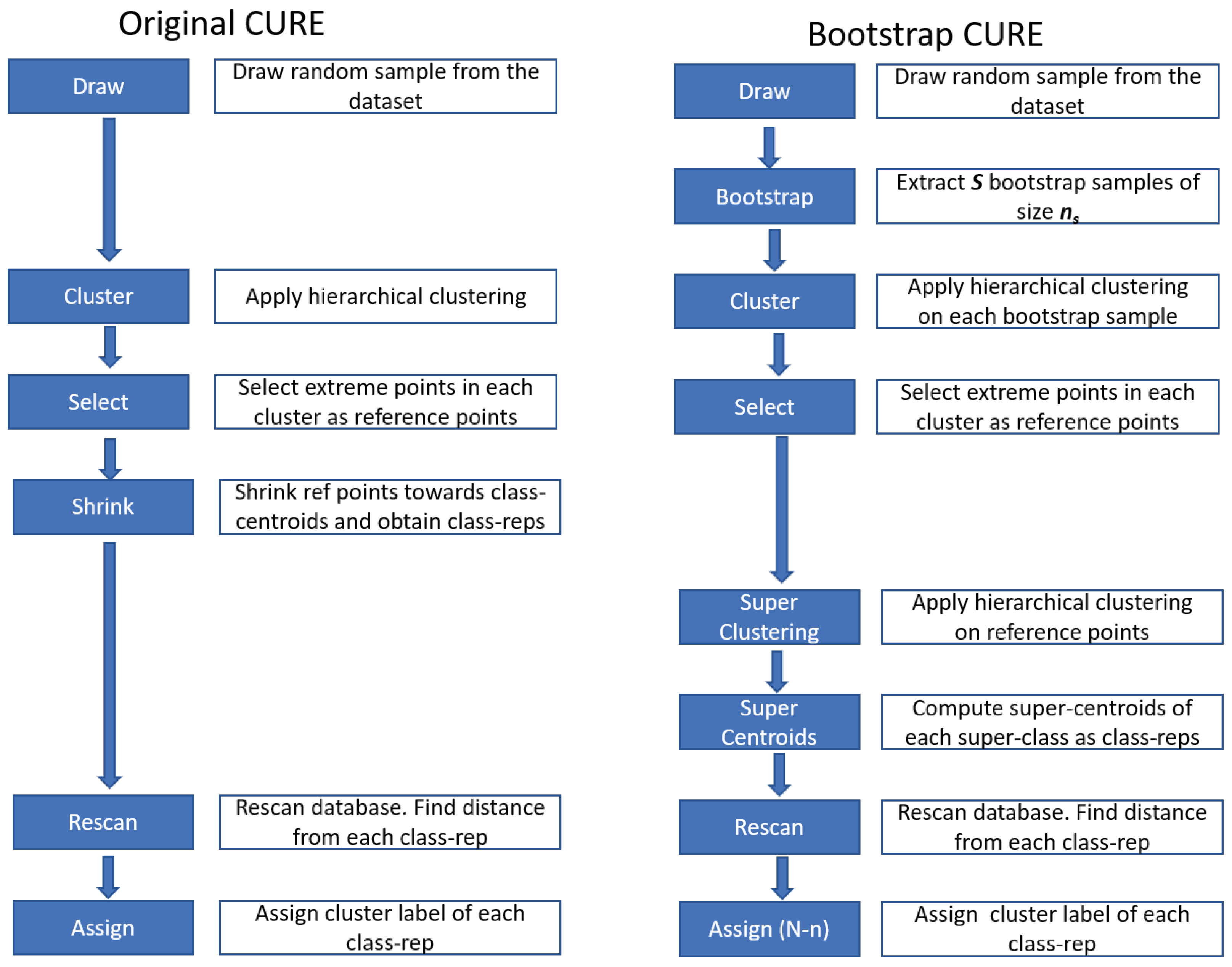
5.1.1. The Proposed Bootstrap–CURE Approach

As said before, the CURE algorithm accelerates the hierarchical clustering processes so as to increase the capacity to deal with bigger datasets, but this is still not sufficient to deal with sensor datasets that provide millions of readings per second.
In this work, a modification of CURE is proposed to overcome this limitation. (Figure 2 shows an overview of the proposal).
The proposed modification is based on the well-known mathematical fact that, given a data set of size n, decomposed in S disjunct subsets of size n s such that
n = s = 1 S n s
then the square of the total size is bigger than or equal to the sum of squares of individual components
n 2 = ( s = 1 S n s ) 2 s = 1 S n s 2
Consequently, any quadratic algorithm running on the entire dataset of size n will be more expensive from the computational point of view than its replication on the S samples. There is no need to run any experiment to demonstrate this property since it is based on an analytical geometrical property of the sum of squares.
This means that applying the bootstrap technique to hierarchical clustering by repeating clustering of small samples from the original dataset several times will surely decrease the complexity of the total process as compared to the global clustering of the entire dataset.
The authors introduce the bootstrap technique in the process in the following. As mentioned earlier, the CURE initialization step in the original definition of the method involves taking a small sample of data, applying hierarchical clustering on it, and further identifying a set of representative points to be used to extend the clusters to the whole dataset. The whole CURE algorithm is based on the idea that the initialization sample is representative of the total population and that other objects assigned in the completion step follow the same cluster structure as the one discovered in the sample. This is quite a strong hypothesis that might not necessarily hold when we are sampling a subset of data, sufficiently small to process hierarchical clustering (quadratic) in a big data dynamic environment. Hence, the authors propose to use the bootstrap principle to extract S small samples ( n s n ) , with n being the size of the original dataset and n s being the size of the sth sample from the initial dataset for the initial clustering step.
This proposal is based on the idea that each sample is clustered under a hierarchical method independently, thus resulting in S dendrograms. A subsequent intermediate step of super classification is proposed as well to encompass the results of independent sample clusters. The super classification performs over the set of class representatives (centroids) coming from all the samples processed and thus the final set of clusters is more robust than the original CURE algorithm and eventually, has better representation and lower computational cost. To assign class labels to the remaining objects, the following steps are followed:
  • Draw S random samples of a single reference dataset I, each of same size n s , without replacement.
  • Subject each sample to hierarchical clustering (in this work with Euclidean distance and Ward’s method), and obtain the S dendrograms.
  • Cut the S sample dendrograms and retrieve a set of clusters for each sample. In Section 5.2, a method to automatically determine the number of clusters in each dendrogram is proposed.
  • Compute the centroid of all clusters found in the previous step and build a final dataset with all centroids.
  • Super-classification step: Apply hierarchical clustering on the centroids dataset.
  • Cut the resulting dendrogram by using the automatic criterion proposed in Section 5.2 and find the set of centroids belonging to each super-class.
  • Compute the super-centroids of each super-class.
  • Retrieve the list of original points belonging to each super-class by finding the centroids belonging to the super-class and the original elements used for each centroid.
  • Assign the label of the corresponding super-class to all elements included in the S samples used.
  • For all the elements that were not part of the S samples, compute the distances to each of the super-centroids.
  • Assign each element the class of the nearest super-centroid.
Figure 2 compares the steps in the original CURE and the proposed bootstrap–CURE methods.

5.2. Determining the Number of Clusters: Calinski–Harabasz Index

In any hierarchical clustering algorithm, the number of clusters emerges after plotting the dendrogram and optimizing both the homogeneity and the distinguishability of the clusters. There is an abundance of works in the literature available, dealing with the evaluation and performance of clustering [97,98,99]. A robust evaluation measure was provided by the Calinski–Harabasz index [76], also popularly known as the variance-ratio method. The Calinski–Harabasz index, for a clustering solution P consisting of k clusters from a dataset having n rows, is calculated as follows:
C H ( k ) = B k / ( k 1 ) W k / ( n k )
where k is the number of clusters. B k is the between classes variability, defined as
B k = C P n C d l ¯ C , l ¯ 2
and W k is the within classes variability, defined as
W k = C P i C d i , i ¯ C 2
l ¯ C is the centroid of the cluster C, n C is the size of cluster C, and l ¯ is the centroid of the whole dataset.
In theory, the number of clusters obtained by using the Calinski–Harabasz method should match with the number of clusters deduced by the experts looking at the dendrogram. In the earlier work by Karna et al. [78], the authors evaluated five different criteria based on the Calinski–Harabasz index over 100 datasets of varying size and assessed the validity of those five criteria in regards to visual inspection by human experts. In practice, a human expert usually finds the best cut of the dendrogram, finding the branches with a wider vertical gap between consecutive nodes. The final clusters correspond to the branches of the tree isolated by the horizontal cut. The result of the experiments performed in [88], however, indicated all criteria based on the Calinski–Harabasz index to be underperforming. It was also evidenced that the Calinski–Harabasz index does not align with real expert practices well enough.
Thus, Suman et al. proposed two new criteria to overcome this limitation based on the heights of the internal nodes of the dendrogram that better follow the real practices performed by experts and prove that the criterion Δ H c o n d is the one that better approaches that of experts. This is the criteria proposed to be included in the general methodology proposed in Section 5.1.1.
Let h ν , ν 1 : n 1 be the height of node ν in a given dendrogram built over a dataset I. The values of h ν depend on the linkage method used in the hierarchical process that generates the dendrogram. The Δ H c o n d [88] is defined as follows:
K Δ H c o n d = K 2 Δ H if K Δ H = 2 and ( h 2 / h r o o t ) > 1 / 3 K Δ H otherwise
where h r o o t and h 2 represent the heights of the two highest nodes of the dendrogram and the K Δ H and K 2 Δ H are the maximum and second maximum of the Δ H criterion as defined in [78]:
K Δ H = argmax 2 k K ( Δ H k ) ; k ( 2 , 3 , K 1 )
where
Δ H k = h k h k + 1 ; k ( 2 , 3 , K 1 )
It is shown empirically that the Δ H criterion underperforms where the best cut of the tree is two clusters, as experts are biased toward this scenario and use a heuristic to skip the two clusters’ cut sometimes. The modified criterion, defined as, The Δ H c o n d incorporates this heuristic by introducing the concept of the height factor as a ratio between the heights of the two highest nodes of the dendrogram. This can be visualized in Figure 3. Here, the tree structure on the right (Figure 3b) represents the annotated dendrogram that reveals that the biggest gap between nodes occurs at K = 2 , where the difference in height between involved nodes is ( 85.5 27.1 = 58.4 ). The second-best clustering solution occurs at K = 4 with the height difference as ( 25.9 19.5 = 6.4 ). In this case, the expert does not go for a solution of K = 4 , but a solution of K = 2 .
At the same time, in Figure 3a, the annotated dendrogram reveals the biggest gap of the tree as occurring at solution K = 2 , the maximum Δ h 1 = 68.5 43 = 25.5 , and the second best solution is seen at K = 3 , Δ h 2 = 43 27.5 = 15.5 . Thus, following the height-factor notion, the second best solution coincides with the expert’s understanding of three clusters.
This corresponds to a practical situation where the cut in two clusters often provides general results, which may not be very interesting from the application point of view, and the second-best cut tends to be preferred by stakeholders, as it is more informative.
The proposed method by Suman et al. [88] shows an impressive result with the Δ H c o n d criterion matching the expert criterion in 93% of tested datasets and performs significantly better than all other criteria, including the proposals in [78].

5.3. Post-Processing: Toward Explaining the Clusters

Once the dataset is clustered, specific assessment tests are used to identify the significant sensors in the clusters according to the methodologies presented in [90]. The class panel graphs (CPG) [89] are used to visualize the behavior of the sensors through the different clusters; properly interpret the results of the tests given in [90] as well as to show how sensors are related with one another; and eventually to induce conceptualization to the experts. The CPG is used to analyze the conditional distribution of sensor data versus clusters. It also helps understand some key patterns among the clusters with respect to sensor behavior. Illustrative variables, which were not part of the original data used in the clustering, are also used to enrich the interpretations.
The proposal of using conditional distributions of sensors toward clusters as a basis to the automatic interpretation of the clusters is based on the post-processing methodologies discussed in [89,100,101], which is directly aligned with the introduction of a knowledge production step on the data mining process as proposed by Fayyad et al. [102]. This approach of interpreting clusters is also aligned with the emerging field of explainable AI [103] by providing conceptual explanations of the discovered patterns. This confers explanatory capabilities to the AI methods, which is one of the fundamental requirements for integrating a data-driven method in an intelligent decision support system.

5.4. Validation of the Proposal

The validation is performed with regards to two different aspects. Firstly, the discovered clusters are validated by adding external information from the job summary that provides a status message for each job as well as the reasons of failure (if available), which is captured separately, analyzing how this external information distributes with the discovered clusters.
Secondly, regarding the benefits of bootstrap–CURE with respect to scalability, the methodology is also validated in terms of computational cost. The total CPU time it takes to cluster a large dataset by the classical hierarchical clustering method and original CURE clustering method is compared against the proposed bootstrap–CURE approach. Hence, the scalability of the algorithm is directly tested by running several experiments of varying dataset sizes, both by the traditional and proposed approaches. The experimental results are discussed in Section 6.5 and Section 6.6.

6. Applications to 3D Printer Data

6.1. Data Collection

The data from eight anonymized HP multi-jet 3D printers were collected for over 300 printing jobs and appended together to create a large dataset comprising sensors’ behaviors toward various internal processes and sub-systems, including pressure, temperature, humidity, etc. A dataset of approximately 562,000 records was thus generated, containing the behavior of the machines in different phases of a print job. For the current study, the focus was given to the print phase only. For experiments, Python 3.6 was used along with standard scientific libraries (Pandas, NumPy, Scipy, Scikit-learn, and Matplotlib). All experiments were conducted on a GPU-enabled, four-core processor, Windows computer with 32 GB memory.

6.2. Data Preprocessing

The data analysis starts with the computation of descriptive statistics and preprocessing of the variables. Preprocessing follows the scheme provided in Section 5.1. After eliminating the redundant and non-informative sensor features, the final dataset contains 46,821 sensor records across 41 sensors. Table 1 contains the final list of sensors considered in the study [9] with anonymous names to maintain confidentiality. Each sensor rules as a variable of the data matrix (one column of the dataset), whereas rows of the dataset represent measurements at a certain time interval (in seconds).

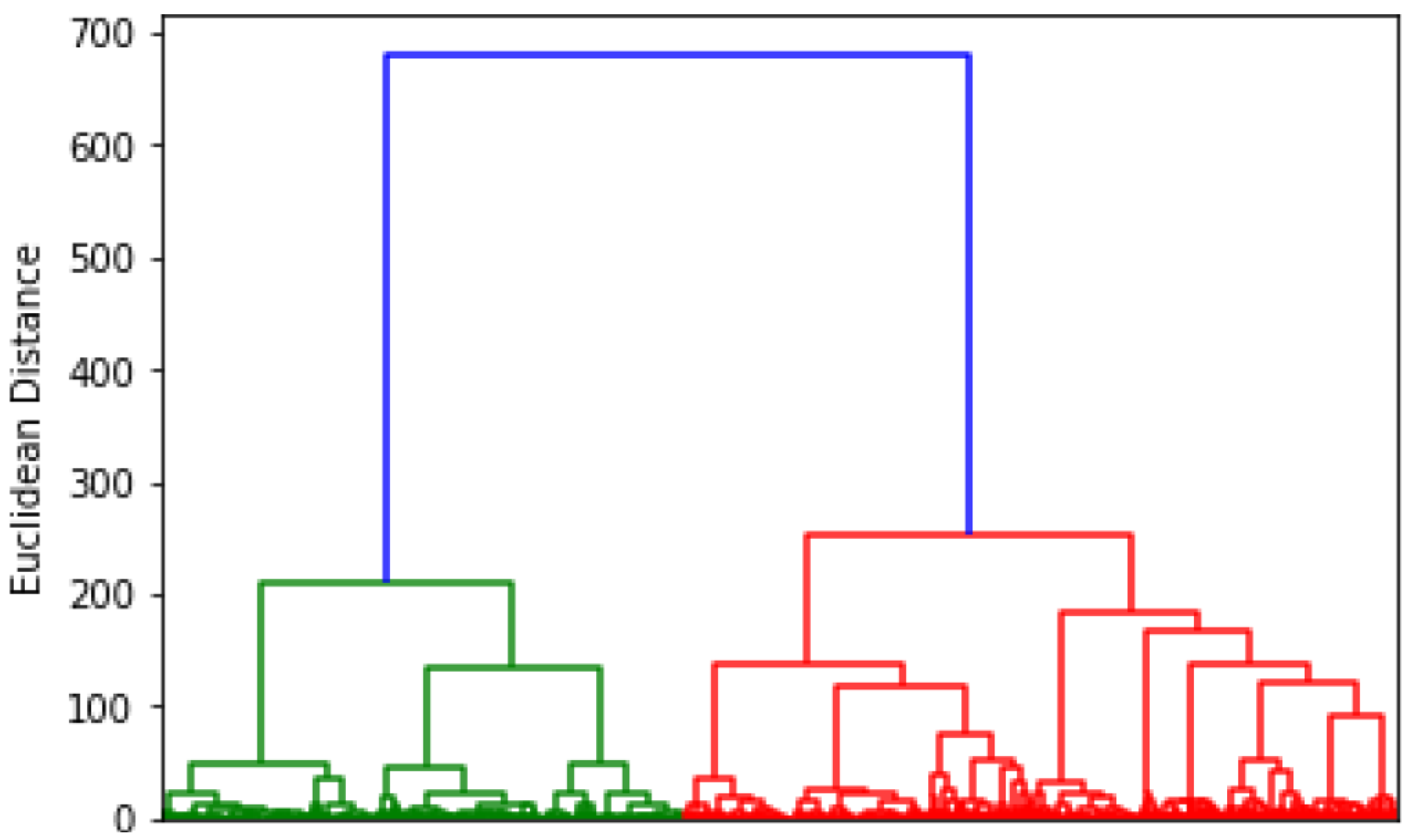
6.3. Hierarchical Clustering

As proposed in Section 5.1.1, the study began with a random sample of 10,000 records drawn without replacement to subject it to hierarchical clustering with Ward’s method. The result was shown in the earlier research work of [9]. Figure 4 shows the corresponding dendrogram.
The four clusters so revealed in the dendrogram were further studied in detail. The use of the class panel graph (Figure 5) helped identify the redundancy among the sensor measurements and drop the redundant variables further to enrich the interpretation.
  • Cluster 0: Specific sensors not meeting the required conditions to print without error.
  • Cluster 1: Shows many sensors reaching the acceptable threshold (to initiate printing).
  • Cluster 2: Conditions associated with print job to fail.
  • Cluster 3: Imbalance in the internal cooling which would result in system error.

6.4. CURE and Bootstrap–CURE

The first step toward the CURE strategy is to shuffle the original data of size n records into a sample of size n = p n , with p being a certain proportion of n. For the bootstrap–CURE, this n size sample is split into r = 10 datasets of size s = n / r records each, drawn at random without replacement. The index of each record from the original dataset was preserved to use them at the later stage of the clustering and to keep the reproducibility of experiments. All 10 sample datasets share the same set of variables as used in work [9] to enable comparisons.
This work continues the application of both CURE and bootstrap–CURE to data according to Section 5.1.1.
For n = 46 , 821 and s = 2000 (and r = 10, so that almost half of the data size is involved in the bootstrap phase and the bootstrap samples have sufficient variability). The dendrograms of some of the samples in the bootstrap process are shown in Figure 6. The proposed approach resulted in a total of 39 centroids (3 centroids from sample_0 and 4 centroids from each of the rest). These 39 centroids merge in a new dataset of final representative points of the clusters. This new dataset of centroids would be subject to the super-clustering step (see Figure 7) in such a way that all centroids across all samples representing the same cluster group are merged. Without going into detail, it is interesting to see that all samples provide more or less similar structures, which are aligned with a good sample representation, even with smaller sample sizes as compared to the size of the complete dataset. As is evident from the dendrograms (Figure 6), all samples (1–9) exhibit 4 cluster structures, except sample_0, which shows 3 clusters.
The final bootstrap–CURE dendrogram (Figure 7) indicates a two-cluster solution; however, as a general practice, a human expert in such a situation often considers the second-best solution which shows four clusters. This strengthens the fact that a four-cluster solution (also established in [9]) is sufficient to represent the sensor behavior in the 3D printer.

6.5. Comparison of Original CURE against Bootstrap–CURE

In order to evaluate the bootstrap–CURE implementation, the algorithm was tested on eight datasets from 3D printers of different sample sizes n, fixed p = 0.5 and r = 10 and the total time to execute CURE and bootstrap–CURE, as well as the hierarchical clustering algorithms, were computed, as shown in Table 2, and a graphical summary was provided (Figure 8).
It is quite evident from Table 2 that as the data grows in size, the original CURE implementation [63] takes quadratically longer CPU time (TCPU). In fact, a quadratic regression between TCPU and sample size provides a single significant coefficient (to the quadratic term) and significant goodness-of-fit coefficient R 2 = 0.9982 .
The proposed bootstrap implementation processes the data quite rapidly, even for a large sample size, and appears to exceed 7× speed for bigger datasets when compared with the classical implementation of the CURE algorithm. The same appears to be up to 40× faster than the hierarchical clustering algorithm in the experiments. This property seems to be well aligned with the goals of Industry 4.0, which require quick automation and analysis of a huge amount of data.
It is also interesting to remark that the automatic criterion to cut the dendrograms developed in [88] was introduced into the process to help automate the entire bootstrap–CURE methodology, which is a great advantage.
From another perspective, the quality of the clusters does not change between CURE and bootstrap–CURE by construction, since the data used for the sampling step are the same in both algorithms; one is clustered together while the other is clustered, divided into 10 samples, and thus is only impacting on TCPU savings but not on the quality of the resulting clusters.

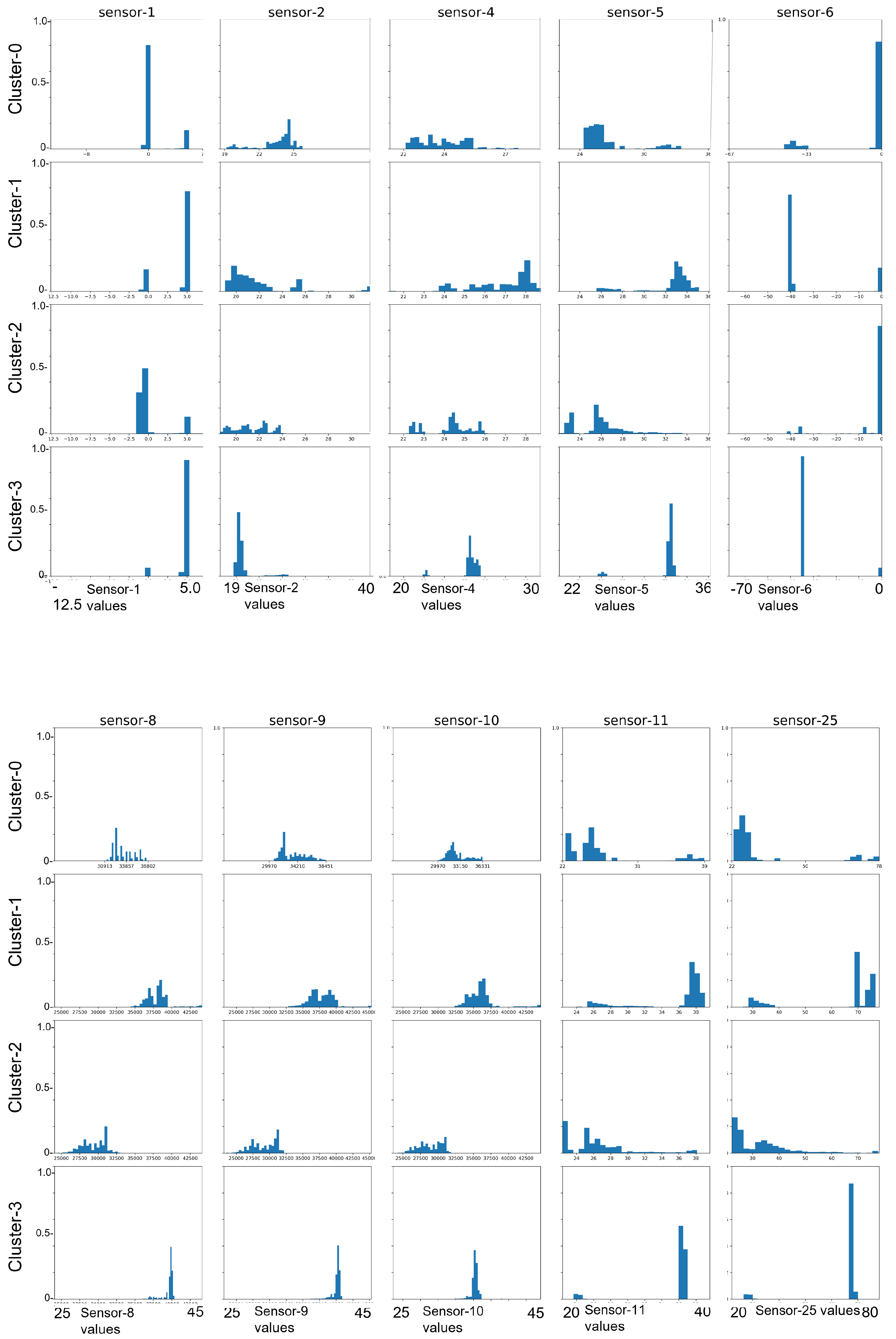
6.6. Post-Processing in Bootstrap–CURE Method

Post-processing of bootstrap–CURE dataset is accompanied with the class panel graph. Figure 9 shows part of the class panel graph from final data (with vertical scales of all cells normalized to a range of [0–1]). The conditional distribution of sensor_1 to sensor_5 exhibits a similar behavior as observed in the work [9].
To compare hierarchical clustering with the bootstrap–CURE strategy, the authors focus on the 10,000 elements common between both experiments. Table 3 shows that class 0 of both clustering approaches is distributed among the other classes, thereby showing some differences in the results for both strategies. The objects included in each cluster are not exactly the same. However, 81.36 % of the printing jobs data match in the same class for both hierarchical clustering and bootstrap–CURE, strengthening our proposal.
Table 4 compares the Calinski–Harabasz (CH) indices between the original sample using the classical hierarchical algorithm, original CURE and the bootstrap–CURE proposal. The C H index obtained on the bootstrap–CURE clustering is much lower than the same obtained in [9], using hierarchical clustering. It is to be noted that the bootstrap–CURE method is computationally much less expensive, as the assignment of labels does not need the whole set of rows to be used in clustering. This is particularly useful to approximate large data by a substantially lesser number of records to process in clustering.
Hence, the profiles discovered by both of the approaches maintain stable clusters; however, the ones obtained by the bootstrap–CURE method are more relevant for the big data framework, as they are based on the larger dataset size and most of the clusters show smaller standard deviations as well. Illustrative variables are also used to help understand the structure of the clusters (see Figure 10 for job status by clusters and Figure 11 for fail reasons by clusters).
Out of 41 sensors, 12 were found to be non-significant subsystems (those referring to sensor_12 through sensor_23), and both sensor_24 and sensor_38 pressure values were found to be constant and, thus, not providing any insight about the printing process. For the remaining 25 sensors, some pairs were found to be redundant according to the clusters, and thus only one of them is considered (sensor_2–sensor_3, sensor_6–sensor_7, and sensor_26–sensor_28) for further study. The remaining 24 variables were analyzed to be following three basic profiles that can be interpreted in detail by analyzing the distribution of sensors.
  • Cluster 0 (non-conformable jobs):
The main characteristics of this cluster are as follows. Firstly, sensor_1 does not reach the recommended pressure for most of the instances and, hence, the job does not start. Sensor_3 shows a higher than expected temperature, which might result in system error. However, sensor_39 shows the measurement within specifications. Thus, the cluster should lead to unsuccessful printing. Further, the cluster is also found to contain several failed jobs with few successful ones, with the most common reasons being failed-to-print and system-error. This aligns with our interpretation based on unsupervised analysis of the cluster data.
  • Cluster 1 (successful jobs):
This cluster is characterized as follows. Sensor_1 has the recommended pressure reading to initiate the job. The temperature measurement in sensor_3 is also adequate as per the domain knowledge, as is sensor_39. In general, the behavior of sensor_39 and sensor_1 should match what is seen in this cluster. Sensor_35 also has the correct measurements; however, sensor_34 does not match the behavior all the time. Hence, this cluster is expected to lead to successful jobs, but there may be a few failures due to a mismatch in the behavior of sensor_35 and sensor_34. Further, analysis of the data reveals that the cluster indeed has mostly successful jobs with few that are ‘failed’ or ‘operator-canceled’. The main reason found for the failure of the job is ‘power-cut’, while some failed to print because an operator canceled the jobs.
  • Cluster 2 (failed jobs due to malfunction of components):
In this cluster, sensor_1 does not reach the recommended pressure value to start the job and this should result in system error. Although the measurements of sensor_3 are within spec, the behavior of sensor_1 and sensor_39 does not match (the pressure values should be reversed to each other), which is evident almost throughout the data. Additionally, sensor_34 shows measurements that are higher than normal. Overall, the cluster shows quite unfavorable readings that would hamper a job to start or would lead to failure. Further analysis revealed that most of the jobs found in this cluster failed with the main reason being ‘system error’.
  • Cluster 3 (failed jobs due to imbalance of sensors):
This cluster is peculiar, as sensor_1 and sensor_3 both are found to be within the recommended specifications, as are sensor_4 and sensor_5. This indicates sufficient conditions for a print job to start. Further, the measurements of sensor_1 and sensor_39 also correspond to each other, which is necessary for a print job to continue. Sensor_34 shows very high readings and thus points to a higher level of humidity; sensor_32 and sensor_33, which control the overall airflow in the machine, run at a lower temperature. This creates an imbalance in the internal cooling environment, which might result in system error. Further verification of the jobs in this cluster disclosed that most of them failed due to ’system error’.

7. Discussion

This paper presents a sensor data science contribution in the field of Industry 4.0 and comprises all steps from the very first of identifying operation modes in a machine monitoring scenario, where large multivariate sensor data are continuously reported. Understanding these operation modes and identifying the patterns of failures can be of interest for further development of statistical models for predictive maintenance, and also to analyze the relationships among other sensors that suggest future improvements in the design of the 3D printer.
It is important to note that the methodology proposed here is general for any large-scale sensor data environment, and this applies to other Industry 4.0 domains, such as gas turbines or air quality in smart cities.
The specific application presented here is with regards to the industrial 3D printers, where customers’ print-layer images or videos are considered confidential, and the method has to rely solely on the sensor data to obtain a global understanding of machine behavior. This is only possible through unsupervised analysis.
In fact, in a real industry context, rapid product innovation makes it difficult to prepare supervised data continuously to learn models. When unsupervised learning is faced, there is no possibility to compute either the misclassification rates or the confusion matrices. To introduce the proposed methodology in a real production environment, the technique must be capable of executing large datasets rapidly in a smart factory setting. The current research identified a bootstrapping-based CURE technique that indeed executes much faster than the traditional methods.
With the help of the proposed methodology, sensor data from the real industrial large 3D printers were analyzed in lesser computational time, and four potential clusters of sensor profiles were discovered. Three of them were associated with print job failure due to different problems, and specific sensors reporting abnormal values were observed. The job summary captured separately is a good resource to validate whether the patterns interpreted from the proposed methodology point to the actual scenarios in the print jobs. Thus, along with the domain knowledge, one can find useful patterns of sensor behavior leading to the overall quality of the print job.
This proposed methodology is unsupervised and scalable to big data frameworks in real-time applications. Compared with the CURE algorithm, without including the proposed bootstrap-based modification, this approach was also found to be very efficient with minimal CPU cost and an increase in speed of up to two orders of magnitude for large datasets. This seems quite promising for Industry 4.0, where such a technique could help retrieve insights from machines or printers with limited computational power rather quickly.

8. Conclusions

In this paper, a new data-science-based intelligent methodology is proposed to assist the management of 3D printers. The work presented in this paper includes three novel contributions.
The main contribution of the proposal is a new scalable hierarchical clustering method, called bootstrap–CURE, which modifies the first step of the original CURE algorithm by introducing a combination of a bootstrap strategy and a super-classification method so that large datasets can be hierarchically clustered. Apart from scaling up the process to large datasets, the impact on the CPU time reduction is also drastic. This provides a new hierarchical-clustering-based algorithm that suitably scales up to the large sensor data and becomes applicable to additive manufacturing. Hierarchical clustering has many advantages, as it is a non-supervised learning method that does not require human intervention. In particular, the hierarchical clustering family does not require any prior hypotheses for the number of clusters, which is extremely useful in additive manufacturing, as, in real cases, users have no a priori idea of the real number of clusters, and it is much better to leave the algorithm to discover it.
Since hierarchical clustering is quadratic, it is not suitable in its original form for large datasets. The proposed bootstrap–CURE method overcomes this limitation and reduces the computational cost drastically by keeping all advantages of the hierarchical clustering.
In addition, a second contribution is a novel criterion to automatically determine the number of clusters from the dendrogram in such a way that the results properly approach what clustering experts find by manual inspection. The proposed criterion is based on the analysis of the level indices of the internal nodes of the dendrograms. Being computationally cheap, this method can be introduced in the bootstrap–CURE strategy without incrementing the computational cost significantly.
This provides a clustering method that is fully automated and can be used with sensor data coming directly from the 3D printers to identify the operational modes of the machines. Finally, the bootstrap–CURE was introduced in a complete data-science methodology to identify those operational modes by obtaining an automatic interpretation of the clusters’ meaning. This provides a very useful decision support tool in the management of 3D printers or complex sensor-equipped machines in general (aero-generators, gas turbines, etc.).
The proposal was tested on real data coming from real 3D printers with very promising results.
For the future, the integration of the proposed method in an intelligent decision support system that can interpret the operation of an entire fleet of machines in real time is in progress. This will help manufacturers to build better predictive maintenance policies or identify possibilities to improve the 3D printers’ design as well. Regarding the proposed algorithm itself, in the current formulation of the bootstrap–CURE approach, the shrinking step (as used in original CURE) is skipped before the integral clustering of all objects since a super-classification process is used with the bootstrap centroids. However, the improvements of implementing the shrinking on top of them will be analyzed in the mid-term. Once the behavior of 3D printers is profiled and interpreted, in the next steps of the research, a reduced subset of significant sensors associated with the different types of failures will be identified, and predictive models will be developed to identify anomalies in advance.

Author Contributions

Conceptualization: A.K. and K.G.; methodology: S.S. and K.G.; validation: S.S. and K.G. and A.K.; resources: A.K.; visualization: S.S.; supervision: K.G. All authors have read and agreed to the published version of the manuscript.

Funding

This work was supported in part by KEMLG-at-IDEAI (UPC) under Grant SGR-2017-574 from the Catalan government.

Conflicts of Interest

The authors declare no conflict of interest. The funders had no role in the design of the study; in the collection, analyses, or interpretation of data; in the writing of the manuscript; or in the decision to publish the results.

Abbreviations

The following abbreviations are used in this manuscript:
CVICluster validity indices
K f Optimal number of clusters using criterion f
h i Height of ith node in dendrogram
h r o o t Height of the root node in dendrogram
CPGClass panel graph
C H Calinksi–Harabasz index
T C P U Total CPU time in seconds
Δ H c o n d Proposed CVI based on dendrogram height

References

  1. Rüßmann, M.; Lorenz, M.; Gerbert, P.; Waldner, M.; Justus, J.; Engel, P.; Harnisch, M. Industry 4.0: The future of productivity and growth in manufacturing industries. Boston Consult. Group 2015, 9, 54–89. [Google Scholar]
  2. Sureshkumar, P.; Rajesh, R. The Analysis of Different Types of IoT Sensors and security trend as Quantum chip for Smart City Management. IOSR J. Bus. Manag. (IOSR-JBM) 2018, 20, 55–60. [Google Scholar]
  3. Kang, H.S.; Lee, J.Y.; Choi, S.; Kim, H.; Park, J.H.; Son, J.Y.; Kim, B.H.; Do Noh, S. Smart manufacturing: Past research, present findings, and future directions. Int. J. Precis. Eng. Manuf.-Green Technol. 2016, 3, 111–128. [Google Scholar] [CrossRef]
  4. Gibert, K.; Rodríguez-Silva, G.; Rodríguez-Roda, I. Knowledge discovery with clustering based on rules by states: A water treatment application. Environ. Model. Softw. 2010, 25, 712–723. [Google Scholar] [CrossRef]
  5. Gibert, K.; Nonell, R. Impact of mixed metrics on clustering. In Iberoamerican Congress on Pattern Recognition; Springer: Berlin/Heidelberg, Germany, 2003; pp. 464–471. [Google Scholar]
  6. Marti-Puig, P.; Blanco-M, A.; Cárdenas, J.J.; Cusidó, J.; Solé-Casals, J. Effects of the pre-processing algorithms in fault diagnosis of wind turbines. Environ. Model. Softw. 2018, 110, 119–128. [Google Scholar] [CrossRef]
  7. Wong, V.K.; Hernandez, A. A Review of Additive Manufacturing. ISRN Mech. Eng. 2012, 2012, 1–10. [Google Scholar] [CrossRef] [Green Version]
  8. Nale, S.B.; Kalbande, A.G. A Review on 3D Printing Technology. Int. J. Innov. Emerg. Res. Eng. 2015, 2, 2394–5494. [Google Scholar]
  9. Karna, A.; Gibert, K. Using Hierarchical Clustering to Understand Behavior of 3D Printer Sensors. Adv. Intell. Syst. Comput. 2020, 976, 150–159. [Google Scholar] [CrossRef]
  10. Chalapathy, R.; Chawla, S. Deep learning for anomaly detection: A survey. arXiv 2019, arXiv:1901.03407. [Google Scholar]
  11. Malhotra, P.; Ramakrishnan, A.; Anand, G.; Vig, L.; Agarwal, P.; Shroff, G. LSTM-based encoder-decoder for multi-sensor anomaly detection. arXiv 2016, arXiv:1607.00148. [Google Scholar]
  12. van Wyk, F.; Wang, Y.; Khojandi, A.; Masoud, N. Real-Time Sensor Anomaly Detection and Identification in Automated Vehicles. IEEE Trans. Intell. Transp. Syst. 2019, 21, 1264–1276. [Google Scholar] [CrossRef]
  13. Sakurada, M.; Yairi, T. Anomaly detection using autoencoders with nonlinear dimensionality reduction. In Proceedings of the MLSDA 2014 2nd Workshop on Machine Learning for Sensory Data Analysis, Gold Coast, QLD, Australia, 2 December 2014; pp. 4–11. [Google Scholar]
  14. Parllaku, F.; Zaman, A.; Shah, F.; Karna, A.; de Pena, S. Using computational intelligence for smart device operation monitoring. In Proceedings of the 2019 International Conference on Computational Intelligence and Knowledge Economy (ICCIKE), Dubai, United Arab Emirates, 11–12 December 2019; pp. 124–129. [Google Scholar]
  15. Karna, A.; Shah, F. Machine Learning Based Approach to Process Characterization for Smart Devices in 3D Industrial Manufacturing. In Proceedings of the 2020 International Conference on Electrical, Communication, and Computer Engineering (ICECCE), Istanbul, Turkey, 12–13 June 2020; pp. 1–6. [Google Scholar]
  16. Ouyang, Z.; Niu, J.; Guizani, M. Improved vehicle steering pattern recognition by using selected sensor data. IEEE Trans. Mob. Comput. 2017, 17, 1383–1396. [Google Scholar] [CrossRef]
  17. Erfani, S.M.; Rajasegarar, S.; Karunasekera, S.; Leckie, C. High-dimensional and large-scale anomaly detection using a linear one-class SVM with deep learning. Pattern Recognit. 2016, 58, 121–134. [Google Scholar] [CrossRef]
  18. Emadi, H.S.; Mazinani, S.M. A novel anomaly detection algorithm using DBSCAN and SVM in wireless sensor networks. Wirel. Pers. Commun. 2018, 98, 2025–2035. [Google Scholar] [CrossRef]
  19. Liu, L.; Guo, Q.; Liu, D.; Peng, Y. Data-driven remaining useful life prediction considering sensor anomaly detection and data recovery. IEEE Access 2019, 7, 58336–58345. [Google Scholar] [CrossRef]
  20. Wulsin, D.; Blanco, J.; Mani, R.; Litt, B. Semi-Supervised Anomaly Detection for EEG Waveforms Using Deep Belief Nets. In Proceedings of the 2010 Ninth International Conference on Machine Learning and Applications, Washington, DC, USA, 12–14 December 2010; pp. 436–441. [Google Scholar] [CrossRef]
  21. Salem, O.; Naseem, A.; Mehaoua, A. Epileptic seizure detection from EEG signal using Discrete Wavelet Transform and Ant Colony classifier. In Proceedings of the 2014 IEEE International Conference on Communications (ICC), Sydney, Australia, 10–14 June 2014; pp. 3529–3534. [Google Scholar] [CrossRef]
  22. Wibisono, A.; Jatmiko, W.; Wisesa, H.A.; Hardjono, B.; Mursanto, P. Traffic big data prediction and visualization using fast incremental model trees-drift detection (FIMT-DD). Knowl.-Based Syst. 2016, 93, 33–46. [Google Scholar] [CrossRef]
  23. Riveiro, M.; Falkman, G. Interactive Visualization of Normal Behavioral Models and Expert Rules for Maritime Anomaly Detection. In Proceedings of the 2009 Sixth International Conference on Computer Graphics, Imaging and Visualization, Tianjin, China, 11–14 August 2009; pp. 459–466. [Google Scholar] [CrossRef]
  24. Salehi, A.; Jimenez-Berni, J.; Deery, D.M.; Palmer, D.; Holland, E.; Rozas-Larraondo, P.; Chapman, S.C.; Georgakopoulos, D.; Furbank, R.T. SensorDB: A virtual laboratory for the integration, visualization and analysis of varied biological sensor data. Plant Methods 2015, 11, 53. [Google Scholar] [CrossRef] [PubMed] [Green Version]
  25. Nowak, R.D. Distributed EM algorithms for density estimation and clustering in sensor networks. IEEE Trans. Signal Process. 2003, 51, 2245–2253. [Google Scholar] [CrossRef]
  26. Kravchik, M.; Shabtai, A. Detecting Cyber Attacks in Industrial Control Systems Using Convolutional Neural Networks. In Proceedings of the 2018 Workshop on Cyber-Physical Systems Security and PrivaCy, Toronto, ON, Canada, 19 October 2018; Association for Computing Machinery: New York, NY, USA, 2018; pp. 72–83. [Google Scholar] [CrossRef] [Green Version]
  27. Dong, B.; Andrews, B. Sensor-based occupancy behavioral pattern recognition for energy and comfort management in intelligent buildings. In Proceedings of the Eleventh International IBPSA Conference, Glasgow, Scotland, 27–30 July 2009; International Building Performance Simulation Association: Vancouver, BC, Canada, 2009; pp. 1444–1451. [Google Scholar]
  28. Hromic, H.; Le Phuoc, D.; Serrano, M.; Antonić, A.; Žarko, I.P.; Hayes, C.; Decker, S. Real time analysis of sensor data for the internet of things by means of clustering and event processing. In Proceedings of the 2015 IEEE International Conference on Communications (ICC), London, UK, 8–12 June 2015; pp. 685–691. [Google Scholar]
  29. Loane, J.; O’Mullane, B.; Bortz, B.; Knapp, R.B. Interpreting presence sensor data and looking for similarities between homes using cluster analysis. In Proceedings of the 2011 5th International Conference on Pervasive Computing Technologies for Healthcare (PervasiveHealth) and Workshops, Dublin, Ireland, 23–26 May 2011; pp. 438–445. [Google Scholar]
  30. Uhlmann, E.; Pontes, R.P.; Laghmouchi, A.; Bergmann, A. Intelligent pattern recognition of a SLM machine process and sensor data. Procedia CIRP 2017, 62, 464–469. [Google Scholar] [CrossRef]
  31. Grasso, M.; Colosimo, B.M. Process defects and in situ monitoring methods in metal powder bed fusion: A review. Meas. Sci. Technol. 2017, 28, 044005. [Google Scholar] [CrossRef] [Green Version]
  32. Grasso, M.; Colosimo, B. A statistical learning method for image-based monitoring of the plume signature in laser powder bed fusion. Robot. Comput.-Integr. Manuf. 2019, 57, 103–115. [Google Scholar] [CrossRef]
  33. Mani, M.; Feng, S.; Lane, B.; Donmez, A.; Moylan, S.; Fesperman, R. Measurement science needs for real-time control of additive manufacturing powder bed fusion processes. Int. J. Prod. Res. 2017, 55, 1400–1418. [Google Scholar] [CrossRef] [Green Version]
  34. Repossini, G.; Laguzza, V.; Grasso, M.; Colosimo, B.M. On the use of spatter signature for in-situ monitoring of Laser Powder Bed Fusion. Addit. Manuf. 2017, 16, 35–48. [Google Scholar] [CrossRef]
  35. Colosimo, B.M.; Grasso, M. Spatially weighted PCA for monitoring video image data with application to additive manufacturing. J. Qual. Technol. 2018, 50, 391–417. [Google Scholar] [CrossRef]
  36. Yuan, B.; Guss, G.M.; Wilson, A.C.; Hau-Riege, S.P.; DePond, P.J.; McMains, S.; Matthews, M.J.; Giera, B. Machine-Learning-Based Monitoring of Laser Powder Bed Fusion. Adv. Mater. Technol. 2018, 3, 1800136. [Google Scholar] [CrossRef]
  37. Salahshoor, K.; Mosallaei, M.; Bayat, M. Centralized and decentralized process and sensor fault monitoring using data fusion based on adaptive extended Kalman filter algorithm. Measurement 2008, 41, 1059–1076. [Google Scholar] [CrossRef]
  38. He, K.; Zhang, Q.; Hong, Y. Profile monitoring based quality control method for fused deposition modeling process. J. Intell. Manuf. 2019, 30, 947–958. [Google Scholar] [CrossRef] [Green Version]
  39. Zang, Y.; Qiu, P. Phase I monitoring of spatial surface data from 3D printing. Technometrics 2018, 60, 169–180. [Google Scholar] [CrossRef]
  40. March, S.T.; Scudder, G.D. Predictive maintenance: Strategic use of IT in manufacturing organizations. Inf. Syst. Front. 2019, 21, 327–341. [Google Scholar] [CrossRef]
  41. Poór, P.; Basl, J.; Zenisek, D. Predictive Maintenance 4.0 as next evolution step in industrial maintenance development. In Proceedings of the 2019 International Research Conference on Smart Computing and Systems Engineering (SCSE), Colombo, Sri Lanka, 28 March 2019; pp. 245–253. [Google Scholar]
  42. Ruiz-Sarmiento, J.R.; Monroy, J.; Moreno, F.A.; Galindo, C.; Bonelo, J.M.; Gonzalez-Jimenez, J. A predictive model for the maintenance of industrial machinery in the context of industry 4.0. Eng. Appl. Artif. Intell. 2020, 87, 103289. [Google Scholar] [CrossRef]
  43. Bonci, A.; Longhi, S.; Nabissi, G.; Verdini, F. Predictive Maintenance System using motor current signal analysis for Industrial Robot. In Proceedings of the 2019 24th IEEE International Conference on Emerging Technologies and Factory Automation (ETFA), Zaragoza, Spain, 10–13 September 2019; pp. 1453–1456. [Google Scholar]
  44. Lin, C.; Hsieh, Y.; Cheng, F.; Huang, H.; Adnan, M. Time Series Prediction Algorithm for Intelligent Predictive Maintenance. IEEE Robot. Autom. Lett. 2019, 4, 2807–2814. [Google Scholar] [CrossRef]
  45. Gibert, K.; Marti-Puig, P.; Cusidó, J.; Solé-Casals, J. Identifying health status of wind turbines by using self organizing maps and interpretation-oriented post-processing tools. Energies 2018, 11, 723. [Google Scholar]
  46. Luo, B.; Wang, H.; Liu, H.; Li, B.; Peng, F. Early Fault Detection of Machine Tools Based on Deep Learning and Dynamic Identification. IEEE Trans. Ind. Electron. 2019, 66, 509–518. [Google Scholar] [CrossRef]
  47. Nguyen, K.T.; Medjaher, K. A new dynamic predictive maintenance framework using deep learning for failure prognostics. Reliab. Eng. Syst. Saf. 2019, 188, 251–262. [Google Scholar] [CrossRef] [Green Version]
  48. der Mauer, M.A.; Behrens, T.; Derakhshanmanesh, M.; Hansen, C.; Muderack, S. Applying sound-based analysis at porsche production: Towards predictive maintenance of production machines using deep learning and internet-of-things technology. In Digitalization Cases; Springer: Berlin/Heidelberg, Germany, 2019; pp. 79–97. [Google Scholar]
  49. Shi, S.; Wang, Q.; Xu, P.; Chu, X. Benchmarking state-of-the-art deep learning software tools. In Proceedings of the 2016 7th International Conference on Cloud Computing and Big Data (CCBD), Macau, China, 16–18 November 2016; pp. 99–104. [Google Scholar] [CrossRef] [Green Version]
  50. HP Jet Fusion 3D 4200 Printer Review 2018 | Industrial 3D Printer Reviews, 0. Available online: https://www.3dbeginners.com/hp-jet-fusion-3d-4200-review/ (accessed on 19 October 2019).
  51. Xu, R.; Wunsch, D. Survey of clustering algorithms. IEEE Trans. Neural Netw. 2005, 16, 645–678. [Google Scholar] [CrossRef] [Green Version]
  52. Gupta, A.; Datta, S.; Das, S. Fuzzy clustering to identify clusters at different levels of fuzziness: An evolutionary multiobjective optimization approach. IEEE Trans. Cybern. 2019, 51, 2601–2611. [Google Scholar] [CrossRef] [Green Version]
  53. Lahmar, I.; Zaier, A.; Yahia, M.; Bouallegue, R. A New Self Adaptive Fuzzy Unsupervised Clustering Ensemble Based On Spectral Clustering. In Proceedings of the 2020 17th International Multi-Conference on Systems, Signals & Devices (SSD), Sfax, Tunisia, 20–23 July 2020; pp. 1–5. [Google Scholar]
  54. Shirkhorshidi, A.S.; Wah, T.Y.; Shirkhorshidi, S.M.R.; Aghabozorgi, S. Evolving Fuzzy Clustering Approach: An Epoch Clustering That Enables Heuristic Postpruning. IEEE Trans. Fuzzy Syst. 2021, 29, 560–568. [Google Scholar] [CrossRef]
  55. Sebastian, A.; Cistulli, P.A.; Cohen, G.; de Chazal, P. Characterisation of Upper Airway Collapse in OSA Patients Using Snore Signals: A Cluster Analysis Approach. In Proceedings of the 2020 42nd Annual International Conference of the IEEE Engineering in Medicine & Biology Society (EMBC), Montreal, QC, Canada, 20–24 July 2020; pp. 5124–5127. [Google Scholar]
  56. Chakraborty, S.; Das, S. Detecting meaningful clusters from high-dimensional data: A strongly consistent sparse center-based clustering approach. IEEE Trans. Pattern Anal. Mach. Intell. 2020. [Google Scholar] [CrossRef]
  57. Gondeau, A.; Aouabed, Z.; Hijri, M.; Peres-Neto, P.; Makarenkov, V. Object weighting: A new clustering approach to deal with outliers and cluster overlap in computational biology. IEEE/ACM Trans. Comput. Biol. Bioinform. 2019, 18, 633–643. [Google Scholar] [CrossRef]
  58. Li, K.; Cao, X.; Ge, X.; Wang, F.; Lu, X.; Shi, M.; Yin, R.; Mi, Z.; Chang, S. Meta-heuristic optimization-based two-stage residential load pattern clustering approach considering intra-cluster compactness and inter-cluster separation. IEEE Trans. Ind. Appl. 2020, 56, 3375–3384. [Google Scholar]
  59. Zhao, X.; Wang, Z.; Gao, L.; Li, Y.; Wang, S. Incremental face clustering with optimal summary learning via graph convolutional network. Tsinghua Sci. Technol. 2021, 26, 536–547. [Google Scholar] [CrossRef]
  60. Menon, V.; Muthukrishnan, G.; Kalyani, S. Subspace clustering without knowing the number of clusters: A parameter free approach. IEEE Trans. Signal Process. 2020, 68, 5047–5062. [Google Scholar] [CrossRef]
  61. Firdaus, S.; Uddin, M. A Survey on Clustering Algorithms and Complexity Analysis. Int. J. Comput. Sci. Issues (IJCSI) 2015, 12, 62. [Google Scholar]
  62. Kuchaki Rafsanjani, M.; Asghari Varzaneh, Z.; Emami Chukanlo, N. A Survey Of Hierarchical Clustering Algorithms. J. Math. Comput. Sci. 2012, 05, 229–240. [Google Scholar] [CrossRef] [Green Version]
  63. Guha, S.; Rastogi, R.; Shim, K. CURE: An efficient clustering algorithm for large databases. Inf. Syst. 2001, 26, 35–58. [Google Scholar] [CrossRef]
  64. Jagadish, H.; Gehrke, J.; Labrinidis, A.; Papakonstantinou, Y.; Patel, J.M.; Ramakrishnan, R.; Shahabi, C. Big data and its technical challenges. Commun. ACM 2014, 57, 86–94. [Google Scholar] [CrossRef]
  65. Kawamoto, T.; Kabashima, Y. Cross-validation estimate of the number of clusters in a network. Sci. Rep. 2017, 7, 3327. [Google Scholar] [CrossRef] [Green Version]
  66. Fu, W.; Perry, P.O. Estimating the number of clusters using cross-validation. J. Comput. Graph. Stat. 2020, 29, 162–173. [Google Scholar] [CrossRef]
  67. McIntyre, R.M.; Blashfield, R.K. A nearest-centroid technique for evaluating the minimum-variance clustering procedure. Multivar. Behav. Res. 1980, 15, 225–238. [Google Scholar] [CrossRef]
  68. Krieger, A.M.; Green, P.E. A cautionary note on using internal cross validation to select the number of clusters. Psychometrika 1999, 64, 341–353. [Google Scholar] [CrossRef]
  69. Overall, J.E.; Magee, K.N. Replication as a rule for determining the number of clusters in hierarchial cluster analysis. Appl. Psychol. Meas. 1992, 16, 119–128. [Google Scholar] [CrossRef]
  70. Tonidandel, S.; Overall, J.E. Determining the number of clusters by sampling with replacement. Psychol. Methods 2004, 9, 238. [Google Scholar] [CrossRef] [PubMed]
  71. Fang, Y.; Wang, J. Selection of the number of clusters via the bootstrap method. Comput. Stat. Data Anal. 2012, 56, 468–477. [Google Scholar] [CrossRef]
  72. Sevilla-Villanueva, B.; Gibert, K.; Sànchez-Marrè, M. Using CVI for understanding class topology in unsupervised scenarios. In Proceedings of the Spanish Association for Artificial Intelligence, Salamanca, Spain, 14–16 September 2016; Springer: Berlin/Heidelberg, Germany, 2016; pp. 135–149. [Google Scholar]
  73. Tibshirani, R.; Walther, G.; Hastie, T. Estimating the number of clusters in a data set via the gap statistic. J. R. Stat. Soc. Ser. B (Stat. Methodol.) 2001, 63, 411–423. [Google Scholar] [CrossRef]
  74. Jung, Y.; Park, H.; Du, D.Z.; Drake, B.L. A decision criterion for the optimal number of clusters in hierarchical clustering. J. Glob. Optim. 2003, 25, 91–111. [Google Scholar] [CrossRef]
  75. Zhou, S.; Xu, Z.; Liu, F. Method for determining the optimal number of clusters based on agglomerative hierarchical clustering. IEEE Trans. Neural Netw. Learn. Syst. 2016, 28, 3007–3017. [Google Scholar] [CrossRef] [PubMed]
  76. Caliński, T.; Harabasz, J. A dendrite method for cluster analysis. Commun. Stat.-Theory Methods 1974, 3, 1–27. [Google Scholar] [CrossRef]
  77. Milligan, G.W. A Monte Carlo study of thirty internal criterion measures for cluster analysis. Psychometrika 1981, 46, 187–199. [Google Scholar] [CrossRef]
  78. Karna, A.; Gibert, K. Automatic identification of the number of clusters in hierarchical clustering. Neural Comput. Appl. 2021, 34, 119–134. [Google Scholar] [CrossRef]
  79. Cowgill, M.C.; Harvey, R.J.; Watson, L.T. A genetic algorithm approach to cluster analysis. Comput. Math. Appl. 1999, 37, 99–108. [Google Scholar] [CrossRef] [Green Version]
  80. Bruzzese, D.; Vistocco, D. Cutting the dendrogram through permutation tests. In Proceedings of the COMPSTAT’2010, Paris, France, 22–27 August 2010; pp. 847–854. [Google Scholar]
  81. Bruzzese, D.; Vistocco, D. DESPOTA: DEndrogram slicing through a pemutation test approach. J. Classif. 2015, 32, 285–304. [Google Scholar] [CrossRef] [Green Version]
  82. Sander, J.; Qin, X.; Lu, Z.; Niu, N.; Kovarsky, A. Automatic extraction of clusters from hierarchical clustering representations. In Proceedings of the Pacific-Asia Conference on Knowledge Discovery and Data Mining, Seoul, Korea, 30 April–2 May 2003; Springer: Berlin/Heidelberg, Germany, 2003; pp. 75–87. [Google Scholar]
  83. Vogogias, A.; Kennedy, J.; Archaumbault, D.; Smith, V.A.; Currant, H. Mlcut: Exploring multi-level cuts in dendrograms for biological data. In Proceedings of the Computer Graphics and Visual Computing Conference (CGVC), London, UK, 10–11 September 2016; Eurographics Association: Bournemouth, UK, 2016. [Google Scholar]
  84. Vogogias, A.; Kennedy, J.; Archambault, D.W. Hierarchical Clustering with Multiple-Height Branch-Cut Applied to Short Time-Series Gene Expression Data. In Proceedings of the 2016 Eurographics Conference on Visualization (EuroVis), Groningen, The Netherlands, 6–10 June 2016; pp. 1–3. Available online: https://diglib.eg.org/handle/10.2312/eurp20161127 (accessed on 19 October 2019).
  85. Sevilla-Villanueva, B.; Gibert, K.; Sànchez-Marrè, M. A methodology to discover and understand complex patterns: Interpreted Integrative Multiview Clustering (I2MC). Pattern Recognit. Lett. 2017, 93, 85–94. [Google Scholar] [CrossRef]
  86. Gibert, K.; Cortés García, C.U. Weighting quantitative and qualitative variables in clustering methods. Mathw. Soft Comput. 1997, 4, 3. [Google Scholar]
  87. Gibert, K.; Valls, A.; Batet, M. Introducing semantic variables in mixed distance measures: Impact on hierarchical clustering. Knowl. Inf. Syst. 2014, 40, 559–593. [Google Scholar] [CrossRef] [Green Version]
  88. Suman, S.; Karna, A.; Gibert, K. Towards Expert-nspired Automatic Criterion to Cut a Dendrogram for Real-Industrial Applications. Artif. Intell. Res. Dev. 2021, 339, 235. [Google Scholar]
  89. Gibert, K.; García-Rudolph, A.; Rodríguez-Silva, G. The Role of KDD Support- Interpretation Tools in the Conceptualization of Medical Profiles: An Application to Neurorehabilitation. ACTA Inform. Medica 2008, 16, 178–182. [Google Scholar]
  90. Gibert, K.; Sevilla-Villanueva, B.; Sànchez-Marrè, M. The role of significance tests in consistent interpretation of nested partitions. J. Comput. Appl. Math. 2016, 292, 623–633. [Google Scholar] [CrossRef]
  91. Adadi, A.; Berrada, M. Peeking Inside the Black-Box: A Survey on Explainable Artificial Intelligence (XAI). IEEE Access 2018, 6, 52138–52160. [Google Scholar] [CrossRef]
  92. Gibert, K.; Horsburgh, J.S.; Athanasiadis, I.N.; Holmes, G. Environmental Data Science. Environ. Model. Softw. 2018, 106, 4–12. [Google Scholar] [CrossRef]
  93. Gibert, K.; Sànchez-Marrè, M.; Izquierdo, J. A survey on pre-processing techniques: Relevant issues in the context of environmental data mining. AI Commun. 2016, 29, 627–663. [Google Scholar] [CrossRef] [Green Version]
  94. Gibert, K.; Izquierdo, J.; Sànchez-Marrè, M.; Hamilton, S.H.; Rodríguez-Roda, I.; Holmes, G. Which method to use? An assessment of data mining methods in Environmental Data Science. Environ. Model. Softw. 2019, 110, 3–27. [Google Scholar] [CrossRef] [Green Version]
  95. Choi, S.S.; Cha, S.H.; Tappert, C.C. A Survey of Binary Similarity and Distance Measures. J. Syst. Cybern. Inform. 2010, 8, 43–48. [Google Scholar]
  96. Jain, A.K. Data Clustering: 50 Years Beyond K-means. In Machine Learning and Knowledge Discovery in Databases; Springer: Berlin/Heidelberg, Germany, 2010; pp. 3–4. [Google Scholar] [CrossRef] [Green Version]
  97. Maulik, U.; Bandyopadhyay, S. Performance evaluation of some clustering algorithms and validity indices. IEEE Trans. Pattern Anal. Mach. Intell. 2002, 24, 1650–1654. [Google Scholar] [CrossRef] [Green Version]
  98. Gurrutxaga, I.; Muguerza, J.; Arbelaitz, O.; Perez, J.M.; Martin, J.I. Towards a standard methodology to evaluate internal cluster validity indices. Pattern Recognit. Lett. 2011, 32, 505–515. [Google Scholar] [CrossRef] [Green Version]
  99. Salvador, S.; Chan, P. Determining the Number of Clusters/Segments in Hierarchical Clustering/Segmentation Algorithms. In Proceedings of the 16th IEEE International Conference on Tools with Artificial Intelligence, Boca Raton, FL, USA, 15–17 November 2004; pp. 576–584. [Google Scholar]
  100. Gibert, K.; Conti, D.; Vrecko, D. Assisting the end-user in the interpretation of profiles for decision support. an application to wastewater treatment plants. Environ. Eng. Manag. J. 2012, 11, 931–944. [Google Scholar] [CrossRef]
  101. Pérez-Bonilla, A.; Gibert, K. Towards automatic generation of conceptual interpretation of clustering. In Iberoamerican Congress on Pattern Recognition; Springer: Berlin/Heidelberg, Germany, 2007; pp. 653–663. [Google Scholar]
  102. Fayyad, U.; Piatetsky-Shapiro, G.; Smyth, P. From data mining to knowledge discovery in databases. AI Mag. 1996, 17, 37. [Google Scholar]
  103. Gunning, D. Explainable artificial intelligence (xai). Def. Adv. Res. Proj. Agency (DARPA) 2017, 2, 2. [Google Scholar] [CrossRef] [PubMed] [Green Version]
Figure 1. Sensor analyses goals.
Applsci 12 02191 g001
Figure 2. Comparison between original and bootstrap–CURE processing.
Applsci 12 02191 g002
Figure 3. (a) Dendrogram of sample 10; (b) dendrogram of sample 31.
Applsci 12 02191 g003
Figure 4. Classical dendrogram suggesting four potential clusters.
Applsci 12 02191 g004
Figure 5. CPG of redundant variables.
Applsci 12 02191 g005
Figure 6. Sample dendrograms in bootstrap method.
Applsci 12 02191 g006
Figure 7. Dendrogram of centroids.
Applsci 12 02191 g007
Figure 8. CPU time comparison.
Applsci 12 02191 g008
Figure 9. Class panel graph for selected sensors.
Applsci 12 02191 g009
Figure 10. Job status across clusters.
Applsci 12 02191 g010
Figure 11. Job failure reasons.
Applsci 12 02191 g011
Table 1. List of sensors.
VariablesDescription
TimestampTimestamp of the sensor recording
Sensor_1To measure pressure in Air release system
Sensor_2To measure Ambient temperature
Sensor_3To measure temperature in cooling system-1
Sensor_4To measure temperature in cooling system-2
Sensor_5To measure temperature in cooling system-3
Sensor_6To detect glass breakage on left fusing system
Sensor_7To detect glass breakage on right fusing lamp
Sensor_8To measure temperature in carriage back
Sensor_9To measure temperature in carriage front
Sensor_10To measure temperature in carriage middle
Sensor_11Internal camera reading
Sensor_12To measure the reference temperature in subsystem–back
Sensor_13To measure the reference temperature in subsystem–front
Sensor_14To measure the reference temperature in subsystem–middle
Sensor_15To measure the temperature in the subsystem–back
Sensor_16To measure the temperature in the subsystem–front
Sensor_17To measure the temperature in the subsystem–middle
Sensor_18To measure the reference temperature in subsystem–back
Sensor_19To measure the reference temperature in subsystem–front
Sensor_20To measure the reference temperature in subsystem-middle
Sensor_21To measure the temperature in the subsystem–back
Sensor_22To measure the temperature in the subsystem–front
Sensor_23To measure the temperature in the subsystem–middle
Sensor_24To check obstruction in pressure system-left
Sensor_25Temperature coefficient sensor
Sensor_26Temp. coefficient for fusing system1–left
Sensor_27Temp. coefficient for fusing system1–right
Sensor_28Temp. coefficient for fusing system2–left
Sensor_29Temp. coefficient for fusing system2–right
Sensor_30Temp. coefficient for camera system
Sensor_31Temp. coefficient for Cooling left air exit
Sensor_32Temp. coefficient for Top heating
Sensor_33Temp. coefficient for right air exit
Sensor_34Humidity sensor for subsystem XX
Sensor_35Temperature sensor for subsystem XX
Sensor_36Connectivity check sensor for fusing system-left
Sensor_37Connectivity check sensor for fusing system–right
Sensor_38To check obstruction in pressure system-right
Sensor_39Sensor in subsystem
Sensor_40Temperature Sensor in subsystem_z1
Sensor_41Temperature Sensor in subsystem_z2
Table 2. CPU time (sec) comparison among hierarchical, CURE and bootstrap–CURE methods.
Data SizeHierarchical ClusteringCUREBootstrap–CURE
500036.2962.9220.578
10,00068.8754.1251.406
15,000101.0948.2972.094
20,000139.62514.253.156
25,000257.37522.1254.187
30,000262.71832.4225.328
35,000274.10947.4696.75
40,000330.39162.7038.062
45,000443.57876.07810.141
Table 3. Cluster evaluation between hierarchical and bootstrap–CURE.
Bootstrap–CURE
Cluster 0Cluster 1Cluster 2Cluster 3
Hierarchical ClusteringCluster_01476549770133
Cluster 1157232400
Cluster 2201026390
Cluster 354001697
Table 4. Calinski–Harbasz index comparison.
AttributesHierarchical ClusteringOriginal CUREBootstrap–CURE
Sample size10,00010,00010,000
No. of clusters444
Calinski–Harabasz9208.01172885.21015198.4981
Publisher’s Note: MDPI stays neutral with regard to jurisdictional claims in published maps and institutional affiliations.

