Article

Order Releasing and Scheduling for a Multi-Item MTO Industry: An Efficient Heuristic Based on Drum Buffer Rope

1
School of Mechanical and Electrical Engineering, Guangzhou University, Guangzhou 510006, China
2
School of Mechanical Science and Engineering, Huazhong University of Science and Technology, Wuhan 430074, China
3
College of Mechanical and Electronic Engineering, Wenzhou University, Wenzhou 325035, China
4
Department of Mechanical Engineering, Capital University of Science and Technology, Islamabad 45750, Pakistan
*
Author to whom correspondence should be addressed.
Appl. Sci. 2022, 12(4), 1925; https://doi.org/10.3390/app12041925
Submission received: 9 January 2022 / Revised: 1 February 2022 / Accepted: 10 February 2022 / Published: 12 February 2022
(This article belongs to the Collection Heuristic Algorithms in Engineering and Applied Sciences)

Abstract

:
Increasing productivity and efficiency in factories with make-to-order (MTO) production systems have attracted growing interest of academia and industry. In MTO companies, efficient order release and schedule are essential for succeeding in today’s marketplace. However, dynamic demand of customers and constrained resources make it difficult to achieve, as well as limiting the profits. Thus, to overcome the problem of order releasing and multi-item scheduling considering the capacity constrained resources investigated, a heuristic approach is proposed based on the drum-buffer-rope (DBR) method. The proposed heuristic is tested on different types of problems based on due date tightness and demand of products. The performance of the proposed heuristic is compared with other famous heuristic methods in literature. End results indicate that the proposed heuristic based on the DBR method outperforms against the other competitors, and it gives more significant results when optimal buffer size is adopted.

1. Introduction

In today’s competitive environment, the manufacturing trend has changed from mass production to mass customization. The demand of customized products and competitive pressure has forced the manufacturers to design a variety of their products [1]. For example, cars and household appliances producers are manufacturing varieties of products on customer demand. These companies make the standard parts of different product models to fulfill customized demand of different models using make-to-order (MTO) policy. In the MTO production environment, the production starts upon receiving the customer orders. The variety of already manufactured product models are also used in the MTO practices. Therefore, MTO helps to decrease the lead time, work in process inventory and finished goods inventory. Usually, customer orders are composed of various models of the products; therefore, multi-item production lines are used to produce different product models. On the other side, the revenue earned from customer orders can be different under different order schedules in a planning horizon. In this situation, companies have a challenging task to select and manage the variety of customer orders and deliver them by the due date.
The decision to accept and reject the order under uncertainty is a challenging task for the MTO companies. The success of an MTO company depends on choosing an order acceptance policy that can maximize the average revenue per unit cost of the capacity [2,3]. In MTO companies, the planning to produce the final product begins when the customer order is received by the company. One of the disadvantages of the MTO companies is that the lead time to fulfill the orders can exceed the due date of orders, and it may result in penalty costs for companies. Order acceptance and scheduling problems have been investigated in literature by many researchers with different optimizing objectives, including minimization of tardiness or minimizing tardiness related penalties [4,5]. Different heuristics and meta-heuristic methods have been developed for order selection and scheduling problem in literature [3,6,7,8]. However, most of the companies are used to sequence the customer orders at a planning level based on the earliest due date (EDD) or first in first out (FIFO) rules, etc. to simplify the process. Moreover, these heuristics have also been employed to optimize the multi-level planning and scheduling problems [9,10,11,12]. Once the scheduling of orders is completed at the planning level, the customer orders are then scheduled according to the material-based grouping or order release-based rules. In real environments, the customer orders are received randomly and demand is uncertain. The accurate demand and the production order release to produce different parts for final products are critical to determine for each planning horizon. Moreover, production order release from the planning level to the scheduling level is critical to give timely order release information. In most of the companies, there is no proper control mechanism that can determine the production order release of the mix model products [13]. Therefore, rescheduling frequently occurs during the production, which can increase the production lead time and cannot give required production in the required time [13,14].
In addition to these problems, in most of the production lines, some resources hit a bottleneck due to insufficient planning. The resources in a bottleneck can limit the production rate, which are known as capacity constrained resources (CCR). Companies try to fully utilize CCR resources to give continuous production with improved production rate or throughput. Therefore, semi-finished parts are stored near CCR in buffer so that CCR resources cannot become idle in case of any failure. Consequently, the CCR can continuously process to make product models by taking already completed parts of the mix of products from buffer. In MTO, the CCR can be a resource which can use semi-finished standard parts of the product models to make customized product models. Moreover, the production of final product models is carried out on a series of machines like a flow shop. The scheduling process on multiple machines to produce standard parts of the product models is significant to cope with the dynamic requirement of the CCR to avoid shortage of the required standard parts of products in the planning horizon. However, in most of the companies, there is no control mechanism that can determine the schedule of parts to produce according to the order release from the planning level. Therefore, it is challenging to determine the production orders release according to the planned schedule of the customer orders for proper synchronization to reduce the rescheduling process.
The drum buffer rope (DBR) method has been employed by various researchers for the material synchronization used by the CCR to produce the customized products [15,16,17,18]. The synchronization can protect the production plans of the CCR resource from disruptions because of breakdown at the upstream resources. For example, a material buffer is placed before CCR to store the required material and, if some uncertain event occurs on the upstream resources, the CCR can have enough material in buffer to continue its production. The DBR method is significant to synchronize the demand of standard parts of the product models to produce with respect to buffer requirements of CCR in each planning horizon. The material buffer that contains standard parts of the mix model of products is continuously used by CCR to make different product models of the randomly arriving orders in each planning horizon. Therefore, the production order release of the standard parts of the product models is changing according to the buffer requirement in each planning horizon. DBR is also significant to give feedback information of the production order release and work in process accordingly in each planning horizon in upstream resources of CCR. The production planning schedule runs according to the need of the buffer because the buffer is used by CCR, which determines the performance of the whole production system. However, the need for a buffer is determined according to the material consumption by the CCR in each planning horizon. In literature, different DBR logics have been defined by researchers for production planning and control of manufacturing systems [19,20]. For example, Russell and Fry [6] presented a DBR method in the MTO environment to give different order review and release policies. Moreover, Sirikri and Yenradee [21] used DBR based production planning and control to determine the relation of buffer sizes with the lead time up to CCR and how it can affect the specific performance measures in a flow shop environment. Furthermore, the DBR method has also been implemented in manufacturing industries [22], including packaging material [23], LCD plants [24], panel fabrication plants [25], and assembly shops for trucks and trailers [26]. In addition, the DBR method has also been implemented in the scheduling of aircrafts, improving labour relations performance [27], etc. de Eulate et al., [28] implemented the DBR approach on multi-manufacturing projects and [29] introduced a dynamic DBR approach for time buffer for production planning and control in two machine capacitated flow shops. However, most of the literature investigated a time buffer that can control the time of release to produce the products, whereas the production release mechanism of standard parts of the mix model products based on the real time usage rate of the buffer on CCR and demand rate of product models in the planning horizon is significant to determine production order release in each planning horizon for MTO companies. This can reduce the production time of customer orders. Moreover, it can generate feedback of production order release of the standard parts of the product models according to the CCR requirement in each planning horizon. Furthermore, the buffer of CCR can be utilized effectively to produce customer orders in the planning horizon of the order schedule, which can give more profit in each planning horizon. Due to significant application of DBR, a novel real-time production order release mechanism is presented in the current research to control standard parts of the variety of product models in buffer before CCR in MTO companies in each planning horizon.
The planning and detailed scheduling of multi-item products in the production lines considering CCR and the continuous production order release information based on the CCR consumption rate in the planning horizon are novel applications of DBR for MTO companies [30], and it is presented in the current research. Furthermore, the novel customer order delivery control method is also presented in the current research to select the customer orders from an order pool and process on CCR based on the net profit in the current planning horizon. Moreover, the model is developed with heuristic steps for scheduling multi-item products from different orders in the production line which are downstream of the buffer and CCR for customer order delivery control. The proposed DBR method considers different conditions, based on which production order release is made for different product models to fill the buffer in each planning horizon. It also helps to obtain an optimal detailed schedule for MTO companies to complete customer orders on time and utilize the CCR to increase the throughput and profit in each planning horizon. Current research is novel in different aspects, which includes:
Introducing a novel DBR based production order release mechanism for mix model production;
Presenting a novel strategy of optimum and flexible order delivery to maximize net profit in each planning horizon;
Proposing a novel heuristic based on DBR for order releasing and multi-item scheduling in an MTO industry.
The rest of the paper is organized as follows: Section 2 illustrates the problem description. Section 3 shows the method proposed in this research. Section 4 consists of computational experiments and results. Section 5 presents the conclusions and future directions of the research.

2. Problem Description

A flexible production line is considered in current research, which is composed of several machines in series to process multiple types of products. Customer orders arrived in the workshop with a variety of demand of products with different due dates. Moreover, each customer can give a distinct amount of profit on different product models and have different penalty costs on delay. In addition, due to the capacity constrained resources (CCR), there is a storage buffer of the semi-finished parts associated with different product models in the buffer near CCR. Different buffer sizes are assigned to each product model to complete the uncertain demand of product models from customers. The problem is concerned to decide the production sequence of different product models on the CCR resource so that the buffer of each product models can be utilized efficiently and the company can earn more profit to fulfill customer demand in each planning horizon. Figure 1 illustrates a schematic of the proposed DBR based rolling horizon concept for order scheduling and mixed model sequencing in the production line.
The objective of the planning and scheduling problem is to maximize the net profit earned from different customers in a planning horizon as indicated in Equation (1):
max   N P = τ = 1 Γ i = 1 I z = 1 Z [ q = 1 d ^ z τ i U P x i X x z q τ i P C x i ( d ^ z τ i q = 1 d ^ z τ i X x z q τ i ) ]
X x z q τ i = { 1 , i f   C o m x z q τ i D D x z q τ i 0 , o t h e r w i s e
C o m x z q τ i , m = q = 1 Q τ t x m z q τ i ,   m = 1 ,   q
C o m x z q τ i , m = C o m x z q τ i , ( m 1 ) + t x m z q τ i ,   q = 1 ,   m ( 2 , M )
C o m x z q τ i , m = m a x { C o m x z q τ i , ( m 1 ) ,   C o m x z ( q 1 ) τ i , m } + t x m z q τ i ,   q > 1 ,   m ( 2 , M )
S x τ > 0 ,   x = 1 , 2 , , models ,   τ = 1 , 2 , Γ
S x τ S C x ,   τ = 1 , 2 , Γ
Equation (1) indicates maximizing the objective of total net profit that can be earned from customer orders from all customers and all planning horizons. The objective function includes unit profit that can be earned from a product model from different customers on the basis of their urgency, etc., and it also includes the penalty cost that the company has to pay to the customer if the demands of the customer are not met before their due date. The penalty cost for each product model is also different for different customers. Equation (2) indicates a binary variable to know if the completion time of the product model is within its due date. Equation (3) to Equation (5) indicate the completion time of any product model on CCR and other downstream machines. Equation (6) indicates that, for any planning horizon, there is always some storage of material related to any product model in the product model buffer of CCR exits. Equation (7) indicates the buffer size constraint of product model x in planning horizon τ .

3. A Drum Buffer Rope Based Heuristic Algorithm

A novel heuristic procedure for rolling horizon order scheduling and multi-item scheduling for the proposed MTO production system is presented in this section. The heuristic is composed of several steps illustrated in Figure 2. The step-wise procedure of the proposed heuristic method is explained in this section.

3.1. Step 1: Assign Customers to the Buffer of Product Models

In each planning horizon, there is a different demand of customers for each product model, and there is limited buffer size of the product models. In the current CCR model, it is assumed that, in the planning horizon, demand from all customers may not be fulfilled from the available buffer, and there is the possibility that some of the demand of customers may have to be planned in the next planning horizon. This selection of product models from different customer orders is based on the demanded quantity of the product models, the unit profit earned from each product models, and the penalty cost that can be required to pay to the customer in case of delay. These factors can describe the selection criteria of customers to deliver different product model demands or the assignment of the buffer of models to different customers. The assignment of different quantities of product models from buffer to different customers is performed using steps shown below:
(i)
Obtain the initial buffer level of each model x in product model buffers in planning horizon τ , i.e., S x τ
(ii)
Obtain the demand of each model x of each customer i in planning horizon τ for CCR, i.e., d x τ i
(iii)
Calculate the net profit of models for each customer based on the demand of customers for each product model in planning horizon τ , i.e., N P x τ i
N P x τ i = U P x i S x τ j = 1 i 1 d ^ x τ j X x τ j P C x i d x τ i S x τ j = 1 i 1 d ^ x τ j X x τ j , i f   d x τ i S x τ j = 1 i 1 d ^ x τ j X x τ j U P x i × d ^ x τ j ,   i f   d x τ i < S x τ j = 1 i 1 d ^ x τ j X x τ j
Z x τ = j = 1 i X x τ j
when d x τ i ( S x τ j = 1 i 1 ( d ^ x τ j × X x τ j ) ) , the demand of model x for customer i is satisfied and the remaining demand is delivered to the next customer and the available buffer of the model continues to be delivered to the customers until the demand from a customer becomes greater than the remaining buffer level of the model in its product buffer.
(iv)
Sort the customers according to their value of net profit N P x τ i for each model.
(v)
Assign the demand of models from S x τ to each customer according to the sorted list based on N P x τ i .
(vi)
Get the total number of lots in the current planning horizon using Equation (10).
Z τ = x = 1 m o d e l s Z x τ

3.2. Step 2: Generate the Schedule of Product Model Lots on CCR and Downstream Machines

The CCR and other downstream machines in the production line producing product models on serially connected machines and makes a permutation flow shop. In the permutation flow shop, the NEH heuristic [31] is significant to make a schedule of different product models for makespan minimization criteria. However, in the current considered problem, the objective to schedule the product model lots is to maximize net profit in each planning horizon. Therefore, a new heuristic procedure is proposed for the scheduling of product model lots on CCR and other downstream machines. The scheduling of product lots on CCR and other downstream machines is obtained using the proposed customer order delivery control heuristic, which consists of steps as listed below:
(i)
Calculate the total production time on downstream machines using Equation (11).
T x τ = m = 1 M ( t x m × d ^ x τ i )   i = 1 , 2 , , I
Here, the machine m = 1 is the CCR or bottleneck machine and M is the number of machines after CCR in the machining line including the CCR machine:
(ii)
Sort d ^ x τ i in decreasing order of T x τ and name the list as L containing y number of different d ^ x τ i .
(iii)
Pick the d ^ x τ i from this list at position j = 1 and insert at j = 1 position in the lot sequence.
(iv)
Pick the d ^ x τ i from this list at y and insert at all possible y number of positions in the lot sequence i.e., insert at position 1 < z Z in sequence and select the partial sequence which gives the maximum value of net profit of the partial sequence. Let j = j + 1 and go to step 4 until y = Z .
If the value of net profit of all the partial sequences is the same, then select the partial sequence which gives less value of makespan among these partial sequences.
(v)
Perform insertion in the sequence until S x τ = 0 for all models in the buffer storage, i.e., buffer level of models in the buffer in planning horizon τ .
(vi)
The total number of products produced can be calculated using Equation (12):
Q τ = i = 1 I x m o d e l s z = 1 Z q = 1 d ^ z τ i X x z q τ i

3.3. Step 3: Net Demand of Models for Production Order Release

In every planning horizon, it is not necessary that the demand of product models of all customer orders is fulfilled from the buffer. Some of the demand of product models of customers is transferred to the next planning horizon if it is not completed in the current planning horizon. Furthermore, the planning horizon can have demand from product models from the current planning horizon and some of the incomplete demand of product models from the previous planning horizon. Therefore, the net demand of product models is necessary to compute. The following step is used to compute net demand of product models in the planning horizon.
Obtain the demand of each model from each customer to schedule on machines upstream of CCR for planning horizon τ = τ + 1 ,
d ¯ x τ i = ( i = 1 I d x ( τ 1 ) i S x ( τ 1 ) ) + d x τ i d i p x ( τ 1 )
( i = 1 I d x ( τ 1 ) i S x ( τ 1 ) ) is the unsatisfied demand of models in the planning horizon τ .

3.4. Step 4: Production Order Release of Product Models

The schedule that can decide the production order release of the product model on the upstream machines of CCR depends on the demand of each product model in the planning horizon and the rate of usage of material of product models from its assigned product buffer on CCR. The proposed procedure has considered the net demand left after each amount of material picked up from the buffer by the CCR. This can give the priority for processing on upstream machines of CCR to the product models which have more demand left and have more usage rate from the buffer.

3.4.1. Demand Ratio

Demand ratio of models indicates the ratio of the net demand remaining for a product model to release in production order with the net demand of the product models excluding work in process product models. This ratio is calculated after each product model produced from CCR to give the priority of the material or production order release for product models based on the remaining net demand:
D R x τ q = d ¯ x τ i q = 1 Q τ X x τ q i = 1 I x = 1 m o d e l   s d ¯ x τ i x = 1 m o d e l   s d i p x ( τ 1 )
The release of models is calculated according to the usage rate of models from buffer and the demand rate of the models from the customer orders in the current planning horizon. The more the demand, the greater will be the priority to release the production order for that product model on the upstream machines of the CCR. Similarly, the greater the usage rate of material from buffer in CCR, the greater will be the requirement of the used material and ultimately the priority will be greater to release the production order for that product model on upstream machines of CCR. The sum of demand ratio and the sum of usage rate of a product model on CCR after each product produced on CCR, L x τ ( q + 1 ) , is termed as production order release pressure. It can determine the production order release for a product model.

3.4.2. Order Release Mechanism

In the DBR model, the buffer is equally divided into three parts with different colors (Red, Yellow, Green) to facilitate buffer management and monitor the state of the whole production system [32]. Zone 3 with a green color means that the buffer is still abundant, so we do not need to take measures for orders, just keep paying a little bit of attention. Zone 2 with a yellow color indicates that the order requires concern. We need to confirm their current location and production status, and take necessary measures. The Zone 1 area with a red color indicates altitude warning. The orders and materials should be tracked and urged immediately to ensure that these jobs and materials reach the buffer zone as soon as possible, to avoid delivery delay.
The order release mechanism based on DBR theory for the current research is indicated in Figure 3. It is supposed that the buffer size B u f x τ is assigned to each product model x independently.
Release the material in sequence according to the L x τ q in sequence position at q for different models which have maximum value of L x τ q among all product models. The product model that will have a higher value of L x τ q after a product q is produced on CCR will be released in the production order release sequence at position q + 1 . It is not necessary that the sequence of production order release on upstream machines of CCR contains q positions of product model sequence due to different demand rate of product models and their different physical sizes of product models and fixed storage capacity of the buffer. Therefore, ( q + 1 ) is considered as a position in the product model sequence of production order release in upstream machines of DBR.

4. Computational Experiments and Results

The current problem is composed of several design parameters that can affect the performance of the production system. The total profit depends on the demand of customers and the completed orders of the customers in the planning horizon. The amount of order completion depends on the production systems’ parameters including the size of buffer allocated for different product models. It is hard for the companies to identify the optimal size of buffers for each product demand and put this buffer near CCR resources or the bottleneck machine. Therefore, there is a requirement for a robust design of experiments that can fulfill the maximum number of customer orders in dynamic demand of product models composed of different order quantities and due dates in each planning horizon.
In this section, first, experiments are performed to test the performance of the proposed DBR method for the scheduling of customer orders considering CCR resources and buffer in the production shop. Later, the tuning of buffer size for different product models is done and design of experiments is made to obtain optimal buffer size of different product models.

4.1. Performance of the Proposed Heuristic Method

In this section, the proposed heuristic base on DBR is used to make the schedule of customer orders on CCR which are arriving in the production system on an every day planning horizon. The performance of the proposed heuristic based on DBR is compared with the famous scheduling methods in literature including NEH [31] and Kalczynski, et al. [33] and CDS [34] heuristic algorithms. These heuristics are famous in flow shop scheduling problems. A production system consisting of five serially connected machines is considered in which of five different product models—A, B, C, D, and E—that are produced. Customer orders are arriving every day with different demand of product models. The data for the example problem are generated randomly and are explained below.

4.1.1. Data Generation for Problem Instances

The specifications of required data for all the considered problems are as follows:
Processing times of product models on each machine are made from DU [5,35].
Defining proper due dates can positively affect the performance [35,36]. Two different factors are introduced to define due dates: tardiness factor (T) and due date range factor (R). The tardiness factor (T) is used to create loose or tight due dates, and T is defined as T = 1 d ¯ / C m a x , where d ¯ is the average due date and C m a x is the maximum completion time of all jobs.
C m a x is considered as the sum of processing time of the demand of product models that are received and that are to be processed from the previous planning horizon in the current planning horizon.
The due date range factor (R) decides the variability of due dates. The range factor (R) is equal to ( d m a x d m i n ) / C m a x , where d m i n is the minimum due date among all customer orders of the product models, and d m a x is the maximum one in a planning horizon τ . Different combinations of T and R can provide different characteristics for randomly generated due dates. In current research, the values of T are considered as 0.85, 0.75, and 0.7 for tight due dates for TS, TM, and TL problems, respectively. Moreover, the values of T are considered as 0.6, 0.5, and 0.4 for loose due dates for LS, LM, and LL problems, respectively. Furthermore, the value of R is set to 0.6 which can provide due date variances. Then, the due dates are uniformly distributed over the interval [ d ¯ R d ¯ ,   d ¯ ] with probability T and over the interval [ d ¯ ,   d ¯ + ( C m a x d ¯ ) R ] with probability ( 1 T ) .
In the current research, there are five serially connected machines in the production shop. NEH and CDS methods which are made to schedule jobs on flow shops are used here to make the schedule of the product models. In the current problem, the customer orders received for one product model is considered as one job with the specific due date. The demand of the customer order that is received in three consecutive days is collectively considered to schedule on five machine flow shops using the NEH and CDS schedule, whereas the customer orders with the respective demand of each product model and due date are scheduled on a daily basis using the proposed heuristic based on the DBR method. NEH, CDS, and proposed heuristic based on the DBR method are coded in Matlab, and all the experiments are performed on the same system.
The products demand and due date of customer orders vary in six different ranges in each experiment. Different types of problems are considered based here on the demand of product models and due date of orders. The due date of customer orders can be tight with small demand (TS), tight due dates with medium demand (TM), and tight due dates with large demand (TL). Moreover, there are three more possibilities of due dates and customer demands, which includes loose due dates with small product demands (LS), loose due dates with medium demand (LM), and loose due dates with larger demands (LL). This combination of demand and due dates makes six different problems. For each problem, in different situations of the demand and due dates, the buffer size of products is required to be optimized. Therefore, in the current study, the experimental parameters for these aforementioned problems are given in Table 1.
The example data for one demand scenario of product models in three consecutive days from different customers received for a TS problem is given in Table 2.
The processing time of product models on different machines, the unit profit on product models and penalty cost on products are given in Table 3.

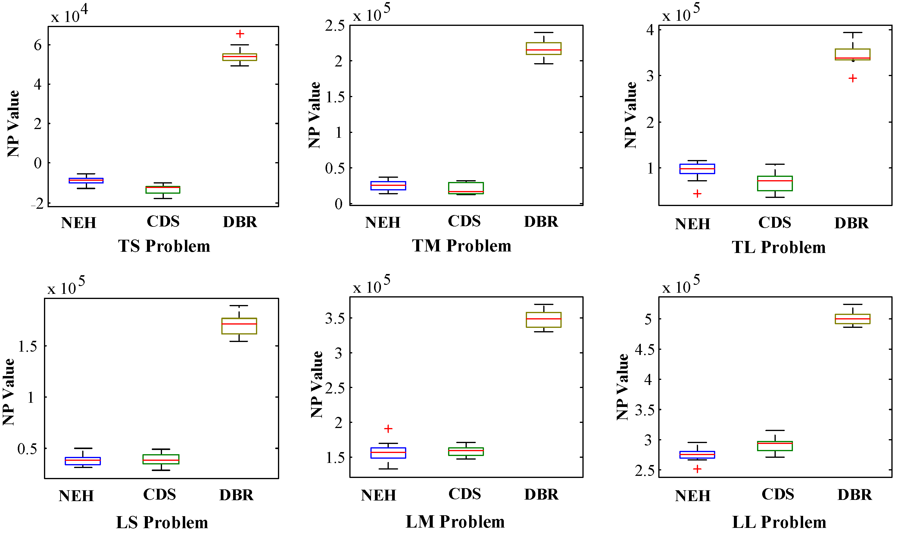
4.1.2. Comparison of Results

The results obtained from the proposed heuristic based on DBR are compared against the results obtained from NEH and CDS heuristic methods based on problem instances of each category of problem. For each problem category, ten different data sets of demand and due date are made from their respective ranges to make ten scenarios that are solved using NEH, CDS, and the proposed DBR based heuristic method. The scheduling results of the product models for each customer based on the NEH, CDS, and DBR based heuristic methods for scenario 1 of problem category TS are illustrated in Figure 4. The results of the schedules of product models of customers based on a three day planning horizon for NEH and CDS algorithms can be seen in Figure 4, whereas the schedule obtained from the proposed heuristic based on the DBR method has a product of customer orders for each day’s planning horizon. These results show that more customer orders can be completed if the proposed heuristic based on DBR is used for scheduling in each planning horizon.
The production order release sequence of product models with the release quantity of the products and the release time obtained from the proposed heuristic based on the DBR method for one scenario of problem category TS for a three day (days 1, 2, and 3) plan are shown in Figure 5.
The results based on the schedule of product models and the customer orders using NEH, CDS, and the proposed heuristic with their NP values for each problem category are presented in Figure 6. The buffer size used for the DBR model is considered as fixed for all problem categories, and the results for NP values of each problem category against 10 different scenarios are presented in Figure 6. It can be seen from Figure 6 that the value of NP for each problem category in different scenarios obtained from the proposed heuristic is higher compared to the NP values obtained from NEH and CDS schedules. This is due to the buffer placed on the CCR machine. Moreover, the buffer can reduce the time of production and can give the products to customers after preparing on CCR and the downstream machines of CCR. Furthermore, the schedule on a daily basis can further increase the possibility of the completion of the customer orders, which gives more NP. This can further increase the value of NP from the proposed DBR method.

4.2. Tuning of Production Systems’ Parameters

In this section, the buffer size for each product model is optimized using the Taguchi method [37]. Different buffer sizes are allocated for each product model in each experiment to test if the considered buffer sizes can complete customer orders on time. These buffer sizes for each product model are the parameters of the production systems which are required to be optimized. For each product model, different levels are considered here which show the buffer size. These levels are made to test various sets of experiments by combining different levels of these parameters. Product models A, B, C, D, and E have buffer sizes of {30, 45, 60}, {30, 40, 50}, {40, 55, 70}, {40, 45, 55}, and {35, 50, 65} for levels 1, 2, and 3, respectively.
The Taguchi method is used in the current study for tuning the system parameters to determine the optimal level of the buffer sizes of each product model. The Taguchi design set of experiment defines levels of the parameters. Buffer size of each product is considered as one experimental parameter for each product model. Therefore, five parameters are taken in the design of the experiment and, for each parameter, three different levels are considered. It contains a total of 27 experiments with different combinations of parameter levels. Signal-to-noise S/N ratio is used to determine the value of the objective function and its variance ratio, which can be used to determine the optimal levels of parameters. In the current experiment design, each problem is tested according to different levels of parameters and the corresponding value of the objective function is computed for each experiment. Once the problem is tested according to the parameters given by the 27 experiments, the mean value of the objective for each parameter is computed for all problems. For example, the mean value of objectives for the parameter ‘buffer size for product model A’ at level 1 is obtained from the first nine experiments. Similarly, mean value for parameter ‘buffer size for product model A’ at level 2 is calculated by taking the average of objective values obtained from the next nine experiments. A similar procedure is employed to obtain the mean value of the objective against each parameter for each level. After that, the mean of means for each level of problems is computed. Furthermore, the measured values that are obtained through experiments are transformed into a signal-to-noise (S/N) ratio. This ratio indicates the amount of variation in the response variable. Based on the current scheduling problem features, the current research applies nominal-is-best. The considered S/N value is calculated using Equation (15):
( S / N ) n o m i n a l = 10 l o g ( m e a n 2 V a r i a n c e 2 )
where (mean)2 and (variance)2 indicate the mean and the variance value of the optimizing objective. S/N values for the considered objective are calculated according to the experiments designed based on the Taguchi method. Then, the mean values of S/N of each objective for all levels of parameters are computed.
In the current case, the level of parameter that gives a higher value of the optimizing objective is preferred because of the maximization objective function. Moreover, the level of parameter at which the maximum value of S/N is obtained is preferred. In the current study, a total of six problem categories based on the demand and due dates are considered and investigated to tune buffer sizes for each product model. Each problem category is tested on ten different customer demand scenarios. Each scenario is tested against 27 experiments as designed in an OA array. The values of NP and values of S/N of NP obtained are averaged against each level of the buffer size. The mean value of NP and mean value of S/N are obtained for each scenario, and these mean values are considered to obtain the mean value of the mean of NP for all ten scenarios of each category of the problem. Similarly, the mean values of the mean of S/N of all 10 scenarios are obtained for each category of problem. The graphical method is used here to obtain the optimal level of buffer size of each product model for each category of problem. Figure 7 shows the mean of mean NP and mean of mean S/N of scenarios against the level of buffers for product models in TS, TM, TL, LS, LM, and LL problems. The optimum levels of buffer size of different product models are obtained by analyzing both mean value of mean NP and mean of S/N values of objectives for each category of problem as given in Table 4.
The optimal buffer size is used for each category of problem. Ten scenarios of each problem category are solved using the proposed optimal buffer sizes in the DBR method. The results obtained for these scenarios for each problem category are compared with the results obtained from the proposed heuristic method with randomly taken buffer sizes for each problem. For each category of problem, ten different scenarios are made and they are solved using the proposed heuristic based on DBR method before and after tuning of the buffer sizes and their NP values are computed. The comparison results of NP values of each problem category using the proposed heuristic before and after using optimal buffer size are illustrated in Figure 8.
It can be seen from Figure 8 that, for different categories of problems, the value of NP is greater when optimal buffer size is used. Moreover, variation in the values of NP in different scenarios is less. These results also indicate the consistency of the results obtained from the proposed heuristic method when optimal buffer size is used, which shows the significance of the proposed heuristic method.
The mean and median value of NP for each problem category before and after tuning of buffer size are calculated and compared as given in Table 5. It can be seen from Table 5 that the mean value of the NP for all categories of problems obtained after buffer size tuning is higher than the NP values obtained before buffer size tuning except for problem LS. Furthermore, Table 5 also indicates the median value obtained from the proposed heuristic method after buffer size tuning is better as compared to the median value of NP obtained before buffer size tuning. These results indicate that the tuning of buffer size for each category of problem can improve the NP value by using the proposed heuristic method.

5. Conclusions

In MTO companies, optimal order scheduling is the golden key to corporate profits. Due to dynamic and uncertain customer demand and constraint resources, it is hard to schedule the customer orders. Therefore, order scheduling and multi-item scheduling problem considering capacity constrained resources (CCR) are investigated in the current research. The novel problem of order scheduling and multi-item scheduling is presented by considering uncertain dynamic demand of products, capacity constrained resource, and a drum buffer rope (DBR) mechanism. A heuristic based on the DBR method is proposed for this problem in a multi-item production environment. The proposed heuristic is adopted to make the customer order delivery schedule in each planning horizon and obtain a production order release sequence for the upstream resources of the production system. The proposed heuristic is tested on different real-life problems. End results indicate that the proposed heuristic method outperforms the other considered heuristics in literature, and it can achieve more significant results.
Uncertainty in the demand of products is considered in the current research. However, in real production shops, various uncertain factors, such as the uncertain variety and processing time, and random arrival time may also exist. Therefore, in future research, these uncertain factors can be introduced to the order scheduling problem. Furthermore, integrating the rule-based heuristics and the intelligent algorithms is also an interesting direction to further improve the performance of the production system.

Author Contributions

Conceptualization, L.Y. and J.M.; Data curation, G.X. and J.M.; Formal analysis, Y.C.; Investigation, Y.C.; Methodology, L.Y. and G.X.; Project administration, T.Z.; Resources, T.Z.; Supervision, T.Z.; Validation, L.Y.; Writing—original draft, L.Y.; Writing—review and editing, L.Y., G.X. and J.M.; Funding acquisition, L.Y. All authors have read and agreed to the published version of the manuscript.

Funding

This research was funded by the Youth Program of National Natural Science Foundation of China (Grant No. 51905196).

Institutional Review Board Statement

Not applicable.

Informed Consent Statement

Not applicable.

Data Availability Statement

Not applicable.

Conflicts of Interest

The authors declare that they have no competing interests.

Notations and Abbreviations

x Index used to represent different product models 0 < x m o d e l s
τ Index used to describe planning horizon 0 < τ Γ
i Index used to represent a customer 0 < i I
m Index used to represent machine
q Index used to represent position of product lot in the order schedule
S x τ Buffer level of model x in buffer in planning horizon τ
t x m z q τ i Processing time of a model x on a machine m
d x τ i Demand of a product model x by a customer i in planning horizon τ
N P x τ i Net profit earned on a product model x from a customer i in planning horizon τ
U P x i Unit profit that can be earned on a product model x from a customer i
d ^ x τ i Lot size of model x for customer i in planning horizon τ
Z τ Total number of lots in planning horizon τ
C o m x z q τ i , m Completion time of product model x of customer i in planning horizon τ which is from a lot z positioned at q on machine m
D D x τ i Due date of product model x of customer i in planning horizon τ
d i p x ( τ 1 ) Quantity of product model x is in process in the machines in planning horizon τ 1
X x z q τ i Binary variable that is equal to 1, if the demand of product model x is completed from lot z , which is at position q in the lot sequence belonging to customer i in planning horizon τ ; otherwise, it is equal to 0

References

  1. Castro, R.F.; Godinho-Filho, M.; Tavares-Neto, R.F. Dispatching method based on particle swarm optimization for make-to-availability. J. Intell. Manuf. 2020, 1–10. [Google Scholar] [CrossRef]
  2. Arredondo, F.; Martinez, E. Learning and adaptation of a policy for dynamic order acceptance in make-to-order manufacturing. Comput. Ind. Eng. 2010, 58, 70–83. [Google Scholar] [CrossRef]
  3. Wu, C.C.; Bai, D.; Zhang, X.; Cheng, S.R.; Lin, W.C. A robust customer order scheduling problem along with scenario-dependent component processing times and due dates. J. Manuf. Syst. 2021, 58, 291–305. [Google Scholar] [CrossRef]
  4. Oguz, C.; Salman, F.S.; Yalçin, Z.B. Order acceptance and scheduling decisions in make-to-order systems. Int. J. Prod. Econ. 2010, 125, 200–211. [Google Scholar] [CrossRef]
  5. Lin, S.-W.; Ying, K.-C. Increasing the total net revenue for single machine order acceptance and scheduling problems using an artificial bee colony algorithm. J. Oper. Reseach Soc. 2013, 64, 293–311. [Google Scholar] [CrossRef]
  6. Russell, G.R.; Fry, T.D. Order review/release and lot splitting in drum buffer-rope. Int. J. Prod. Res. 1997, 35, 827–845. [Google Scholar] [CrossRef]
  7. Abdel-Basset, M.; Mohamed, R.; Abouhawwash, M.; Chakrabortty, R.K.; Ryan, M.J. A simple and effective approach for tackling the permutation flow shop scheduling problem. Mathematics 2021, 9, 270. [Google Scholar] [CrossRef]
  8. Khalid, Q.S.; Arshad, M.; Maqsood, S.; Jahanzaib, M.; Babar, A.R.; Khan, I.; Mumtaz, J.; Kim, S. Hybrid particle swarm algorithm for products scheduling problem in cellular manufacturing system. Symmetry 2019, 11, 729. [Google Scholar] [CrossRef] [Green Version]
  9. Mumtaz, J.; Guan, Z.; Yue, L.; Wang, Z.; Ullah, S.; Rauf, M. Multi-level planning and scheduling for parallel PCB assembly lines using hybrid spider monkey optimization approach. Ieee Access 2019, 7, 18685–18700. [Google Scholar] [CrossRef]
  10. Xu, G.; Guan, Z.; Yue, L.; Mumtaz, J.; Liang, J. Modeling and optimization for multi-objective nonidentical parallel machining line scheduling with a jumping process operation constraint. Symmetry 2021, 13, 1521. [Google Scholar] [CrossRef]
  11. Mumtaz, J.; Guan, Z.; Yue, L.; Zhang, L.; He, C. Hybrid spider monkey optimisation algorithm for multi-level planning and scheduling problems of assembly lines. Int. J. Prod. Res. 2020, 58, 6252–6267. [Google Scholar] [CrossRef]
  12. Yue, L.; Chen, Y.; Mumtaz, J.; Ullah, S. Dynamic mixed model lotsizing and scheduling for flexible machining lines using a constructive heuristic. Processes 2021, 9, 1255. [Google Scholar] [CrossRef]
  13. Zhong, R.Y.; Huang, G.Q.; Lan, S.; Dai, Q.Y.; Zhang, T.; Xu, C. A two-level advanced production planning and scheduling model for RFID-enabled ubiquitous manufacturing. Adv. Eng. Inform. 2015, 29, 799–812. [Google Scholar] [CrossRef]
  14. Thurer, M.; Stevenson, M. Bottleneck-oriented order release with shifting bottlenecks: An assessment by simulation. Int. J. Prod. Econ. 2018, 197, 275–282. [Google Scholar] [CrossRef] [Green Version]
  15. Goldratt, E.M.; Schragenheim, E.; Ptak, C.A. Necessary but not sufficient: A theory of constraints business novel. IIMB Manag. Rev. 2001, 4, 320–323. [Google Scholar]
  16. Telles, E.S.; Lacerda, D.P.; Morandi, M.; Piran, F. Drum-buffer-rope in an engineering-to-order system: An analysis of an aerospace manufacturer using data envelopment analysis (DEA). Int. J. Prod. Econ. 2019, 222, 107500. [Google Scholar] [CrossRef]
  17. Puche, J.; Costas, J.; Ponte, B.; Pino, R.; David, D. The effect of supply chain noise on the financial performance of kanban and drum-buffer-rope: An agent-based perspective. Expert Syst. Appl. 2019, 120, 87–102. [Google Scholar] [CrossRef] [Green Version]
  18. Saif, U.; Guan, Z.; Wang, C.; He, C.; Yue, L.; Mirza, J. Drum buffer rope-based heuristic for multi-level rolling horizon planning in multi item production. Int. J. Prod. Res. 2019, 57, 3864–3891. [Google Scholar] [CrossRef]
  19. Lee, J.-H.; Chang, J.-G.; Tsai, C.-H.; Li, R.-K. Research on enhancement of TOC simplified drum-buffer-rope system using novel generic procedures. Expert Syst. Appl. 2010, 37, 3747–3754. [Google Scholar] [CrossRef]
  20. Thurer, M.; Stevenson, M. On the beat of the drum: Improving the flow shop performance of the drum-buffer-rope scheduling mechanism. Int. J. Prod. Res. 2018, 56, 3294–3305. [Google Scholar] [CrossRef] [Green Version]
  21. Sirikri, V.; Yenradee, P. Modified drum-buffer-rope scheduling mechanism for a non-identical parallel machine flow shop with processing time variation. Int. J. Prod. Res. 2006, 44, 3509–3531. [Google Scholar] [CrossRef]
  22. Benavides, M.B.; van Landeghem, H. Implementation of S-DBR in four manufacturing SMEs: A research case study. Prod. Plan. Control 2015, 26, 1110–1127. [Google Scholar] [CrossRef]
  23. Riezebos, J.; Korte, G.J.; Land, M.J. Improving a practical DBR buffering approach using workload control. Int. J. Prod. Res. 2003, 41, 699–712. [Google Scholar] [CrossRef]
  24. Wu, H.-H.; Chen, C.-P.; Tsai, C.-H.; Yang, C.-J. Simulation and scheduling implementation study of TFT-LCD Cell plants using Drum–Buffer–Rope system. Expert Syst. Appl. 2010, 37, 8127–8133. [Google Scholar] [CrossRef]
  25. Darlington, J.; Francis, M.; Found, P.; Thomas, A. Design and implementation of a drum-buffer-rope pull-system. Prod. Plan. Control 2014, 26, 489–504. [Google Scholar] [CrossRef]
  26. Pegels, C.C.; Watrous, C. Application of the theory of constraints to bottleneck operation in a manufacturing plant. J. Manuf. Technol. Manag. 2005, 16, 302–311. [Google Scholar] [CrossRef]
  27. Chkravorty, S.S.; Hales, D.N. Improving labour relations performance using a simplfied drum buffer rope (S-DBR) technique. Prod. Plan. Control. 2015, 27, 102–113. [Google Scholar] [CrossRef] [Green Version]
  28. De Eulate, U.A.P.; Aiastui, A.L. Application of the DBR approach to a multi-project manufacturing context. In Project Management and Engineering Research; Springer: Cham, Switzerland, 2021; pp. 131–145. [Google Scholar]
  29. Georgiadis, P.; Polituou, A. Dynamic drum-buffer-rope approach for production planning and control in capacitated flow-shop manufacturing systems. Comput. Ind. Eng. 2013, 65, 689–703. [Google Scholar] [CrossRef]
  30. Gilmore, J.H.; Pine, B.J. The four faces of mass customization. Harv. Bus. Rev. 1997, 75, 91–102. [Google Scholar]
  31. Nawaz, M.; Enscore, E.E., Jr.; Ham, I. A heuristic algorithm for the m-machine, n-job flow-shop sequencing problem. OMEGA Int. J. Manag. Sci. 1983, 11, 91–95. [Google Scholar] [CrossRef]
  32. Schragenheim, E.; Dettmer, H.W. Manufacturing at Warp Speed; CRC Press: Boca Raton, FL, USA, 2000. [Google Scholar]
  33. Kalczynski, P.J.; Kamburowski, J. On the NEH heuristic for minimizing the makespan in permutation flow shops. Omega 2007, 35, 53–60. [Google Scholar] [CrossRef]
  34. Ramanan, T.R.; Sridharan, R.; Shashikant, K.S.; Haq, A.N. An artificial neural network based heuristic for flow shop scheduling problems. J. Intell. Manuf. 2011, 22, 279–288. [Google Scholar] [CrossRef]
  35. Bozorgirad, M.A.; Logendran, R. Sequence-dependent group scheduling problem on unrelated-parallel machines. Expert Syst. Appl. 2012, 39, 9021–9030. [Google Scholar] [CrossRef] [Green Version]
  36. Zandieh, M.; Karimi, N. An adaptive multi-population genetic algorithm to solve the multi-objective group scheduling problem in hybrid flexible flow shop with sequence-dependent setup times. J. Intell. Manuf. 2011, 22, 979–998. [Google Scholar] [CrossRef]
  37. Taguchi, A.; Schüth, F. Ordered mesoporous materials in catalysis. Microporous Mesoporous Mater. 2005, 77, 1–45. [Google Scholar] [CrossRef]
Figure 1. Order releasing and scheduling for a multi-item MTO industry in the production line.
Applsci 12 01925 g001
Figure 2. Steps of the proposed heuristic algorithm.
Applsci 12 01925 g002
Figure 3. Order release mechanism based on DBR.
Applsci 12 01925 g003
Figure 4. The scheduling results of the product models for each customer based on NEH, CDS, and heuristic based on the DBR method.
Applsci 12 01925 g004
Figure 5. Order releasing and multi-item scheduling in the rolling three day planning horizon.
Applsci 12 01925 g005
Figure 6. NP results for each category of problem in different scenarios.
Applsci 12 01925 g006
Figure 7. Mean of mean NP and mean of mean S/N of scenarios against levels of buffer size for TS, TM, TL, LS, LM, and LL problems.
Applsci 12 01925 g007
Figure 8. NP value for different categories of problems after and before using the optimal buffer size.
Applsci 12 01925 g008
Table 1. Problem types based on demand and due dates.
Problem CategoryRange of Demand
ABCDE
TS(0~30)(0~40)(0~45)(0~35)(0~40)
TM(30~50)(40~50)(45~60)(35~45)(40~60)
TL(50~70)(50~60)(60~75)(45~60)(60~80)
LS(0~30)(0~40)(0~45)(0~35)(0~40)
LM(30~50)(40~50)(45~60)(35~45)(40~60)
LL(50~70)(50~60)(60~75)(45~60)(60~80)
Table 2. Demand of product models from different customers received on three consecutive days.
Problem CategoryScenarioDayCustomerDemand of Product ModelProbability of
Due Date
TS1 ABCDET = 0.85R = 0.15
111822232298953926
22223832397664901
325312361510622821
21414210117195581
29182903311023549
316341515212961852
315261431413795702
2292131341111992646
312183428412343287
Table 3. Processing time of the product models on different machines.
Product ModelProcessing Time on MachineUnit Profit from CustomerPenalty Cost from Customer
12345123123
A972997150300200153020
B1319321319250200240252024
C82133821350250300352530
D3233343233200350300203530
E2329332329300150250301525
Table 4. Optimum level of buffer size of product models against each category of problem.
Product ModelsOptimum Level of Buffer Size of Product Models for Problem Category
TSTMTLLSLMLL
A332223
B233322
C133232
D333323
E232332
Table 5. Mean and median NP value of each category of problems for before and after buffer size tuning.
Problem CategoryBefore Buffer Size TuningAfter Buffer Size Tuning
Mean NPMedian NPMean NPMedian NP
TS54,231.6654,115.565,591.0963,926.4
TM212,368.9214,561260,831.2261,927
TL340,871339,523352,721.7352,416.5
LS172,125.6171,167.5147,719.5147,140
LM348,834.2348,645.5375,848.3377,246.8
LL500,176.5498,802538,598.2540,171.5
Publisher’s Note: MDPI stays neutral with regard to jurisdictional claims in published maps and institutional affiliations.

