A Scheduling Approach for the Train-Set Circulation Plan and Timetable for the Longer Distance High-Speed Railway in Transition Time

Abstract

Nowadays, high-speed railway (HSR) has become one of the main choices for passengers. As the number of passengers increases, their travel demands become diverse and the fluctuation range of passenger travel demands will also increase. In order to adapt to the change of passenger travel demands, the switching frequency of timetables needs to be increased. When switching the timetable, the train-set circulation plan also needs to be considered. In this paper, a scheduling approach for quickly solving the timetable and the train-set circulation plan in the transition time is proposed. A section sequence is constructed in the integer programming model, and the primary train-set circulation plan is obtained. Then a stop plan is obtained on the basis of passenger travel demands. To obtain the final train-set circulation plan and the timetable, a genetic algorithm (GA) is designed, and a method that can ensure that the timetable meets the safety operation requirements is proposed. The scheduling approach is tested on the Beijing-Shanghai HSR. The results show that by extending the transition time, the scheduling approach can switch the train-set position from the old state to new state, without additional consumption of resources, on the premise of meeting the travel demands of passengers.

1. Introduction

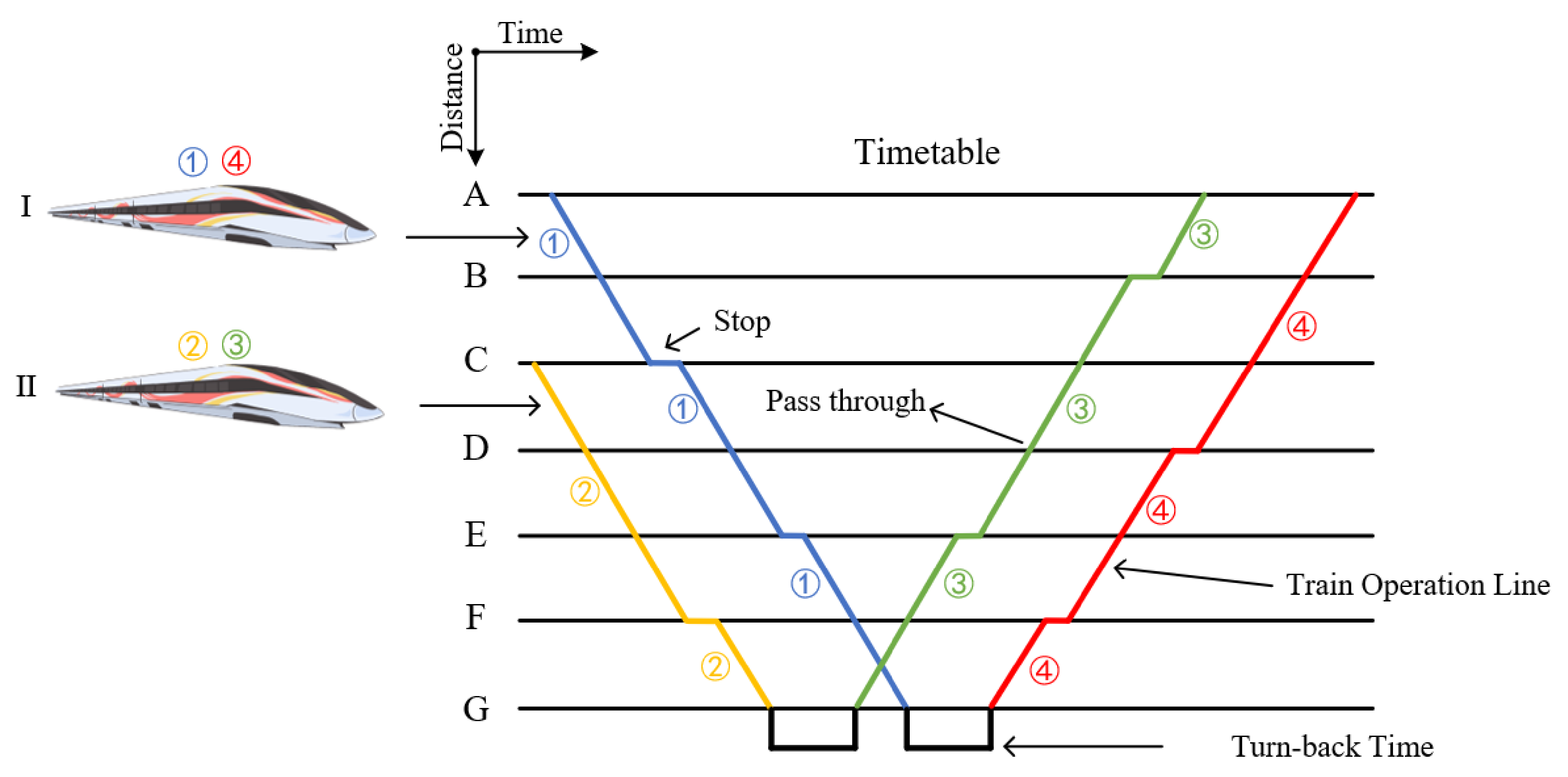
In recent years, the network scale of HSR has developed rapidly, and the length of the HSR line also increased. More and more passengers are choosing to travel by HSR. As the number of HSR passengers has increased, some new operational requirements have emerged. In normal times, the demand for passengers to travel by HSR does not fluctuate much. However, the demand fluctuates because of holidays or special activities. Train timetables are designed to meet the travel demands of passengers, which state the departure time and the arrival time of all train operation lines. HSR operation departments need to change the HSR train timetable in time to respond to the travel demands of passengers. Timely adjustment of the timetable according to the number of passengers can make the arrangement of the operation department more aligned with the demands of passengers, and save the cost of operating a railway line for the operation department. The train timetable contains relevant operational plans, such as train-set circulation plans. The train-set circulation plan is a part of the train timetable, which is a detailed plan of how to use the train-sets when implementing the timetable. The schematic diagram of train-set circulation plan is shown in Figure 1.

As shown in Figure 1, there are four train operation lines in the timetable, representing four operation tasks. A train-set can only perform one operation at a time. Train-set 1 performs operation line 1 first, and train-set 2 performs operation line 2. After the completion of one operation line, the train needs a period to replenish materials and clean the carriage, to perform the next operation line. This period is called the turn-back time. We can see that one train-set can perform multiple tasks in one day. Train-set 1 will perform operation line 4 after completing operation line 1. Similarly, train-set 2 will perform operation line 3 after completing operation line 2. As a result, a timetable requires fewer train-sets than the operation lines it contains. Such a plan containing the corresponding relationship between train-set and operation line is called a train-set circulation plan. Passengers need to get on or off the train, so, train-set needs to stop at a station to serve passengers. If a train-set does not stop at the station, we call the train-set pass through the station.

When the old timetable is switched to the new timetable, the operation plan related to the timetable also needs to be switched. For the operation department, the number of train-sets required by each station to implement the new timetable may be different from the old timetable. This means that in terms of the location of the train-set, each station has two states. The state after the implementation of the old timetable is the old state, and the state required by the implementation of the new timetable is called the new state. The schematic diagram of the old state and the new state is shown in Figure 2.

In Figure 2 we can see that in the old state, station A has two train-sets and station G has three train-sets. However, in the new state, station A needs three train-sets and station G only needs two train-sets. The time between the end time of the old timetable and the start time of the new timetable is called transition time. To meet the number requirement of train-sets in each station in the new timetable, the operation department has two methods. The first is to use spare train-sets to perform operation lines (method 1). Second, at the end of the day, trains will be transferred from nearby stations that have more train-sets to those that lack them (method 2). The schematic diagram of the timetable switching method is shown in Figure 3.

Figure 2. The schematic diagram of the old state and the new state.

Figure 2. The schematic diagram of the old state and the new state.

Figure 3. The schematic diagram of the timetable switching method.

Figure 3. The schematic diagram of the timetable switching method.

As shown in Figure 3, there is a spare train-set in station G and station A is short of a train-set. To make up for this train-set, the backup train-set at station A can be used, or the spared train-set can be transferred from station G to station A during the transition time. The advantage of the first method is that the train does not need to run empty after the end of the operation, so, it will not result in an increase in operating costs and the waste of resources. The disadvantage is that it will occupy the standby train, which will affect the robustness of the timetable in the implementation process. If there is an emergency, the number of standby train-set may be insufficient, which will expand the negative impact. The advantage of the second method is that it will not affect the robustness in the timetable implementation process, but the disadvantage is as mentioned above, which will cause the waste of resources.

In the past, the train timetable was adjusted infrequently, perhaps only a few times a year. Under this adjustment frequency, there is little difference between the two methods. However, as the number of passengers who chose to travel by HSR increased significantly, the fluctuation range of the number of passengers has increased too. In this case, the previous operation mode of only changing the timetable a few times a year has a large lag relative to passenger travel demands. In order to meet the travel demands of passengers better and save the cost of the operation department, it is necessary to increase the adjustment frequency of the train timetable. The increase in the frequency of train timetable adjustment will amplify the disadvantages of the above two modes, resulting in increased waste of resources or greatly affecting the robustness in the process of timetable implementation.

How to avoid the disadvantages of the above two methods and meanwhile scheduling the train-sets, is a problem that is worth studying, because saving resources while meeting the travel demands of passengers is of great significance for practical applications. Thus, we proposed an approach to extend the transition time. In this approach, we extend the transition time from a few hours to a day and realize the train-set rescheduling from the old state to new state through a one-day operation. We call the operation plan during the transition time the transition timetable. The transition timetable proposed in this paper is an approach for the HSR operation department to transition from the old timetable to the new timetable through the operation. The new timetable and the old timetable have been determined by the operation department. The transition timetable scheduling is a train timetabling problem (TTP), and the relevant train-set circulation plan scheduling is a train-set rescheduling problem (TRP). In the scenario proposed in this paper, the TRP has a higher priority, to avoid the disadvantages of the above two methods.

Both train timetabling problem (TTP) and train-set rescheduling problem (TRP) are complex for long distance HSR lines:

Firstly, train timetables are designed to meet the travel demands of passengers. For the long distance HSR line, the passenger travel demands are more complex. The demand that passengers travel from the origin station to the destination station is called O-D. For example, the number of types of O-D for an HSR line with six stations is:

$$C_6^2=15$$

(1)

Let $n$ be the quantity of stations of the HSR line, the number of O-D types is:

$$C_n^2=\frac{n\times \left(n-1\right)}{2}$$

(2)

Obviously, with the increase in the quantity of stations along the HSR line, the types of O-D increase too. For the long distance HSR line, there are more than twenty stations and there will be more than 300 types of O-D.

Secondly, there are more passengers on the long distance HSR line. The operation department needs to prepare more train-sets to meet the travel demands of passengers. Thus, the complexity of scheduling a train-set circulation plan is higher than a normal railway line.

Thirdly, due to the increasing adjustment frequency of timetables, the requirement of solving efficiency is higher than that of the past. However, the TRP and the TTP are more difficult to solve due to the scale of the problem in long distance HSR lines.

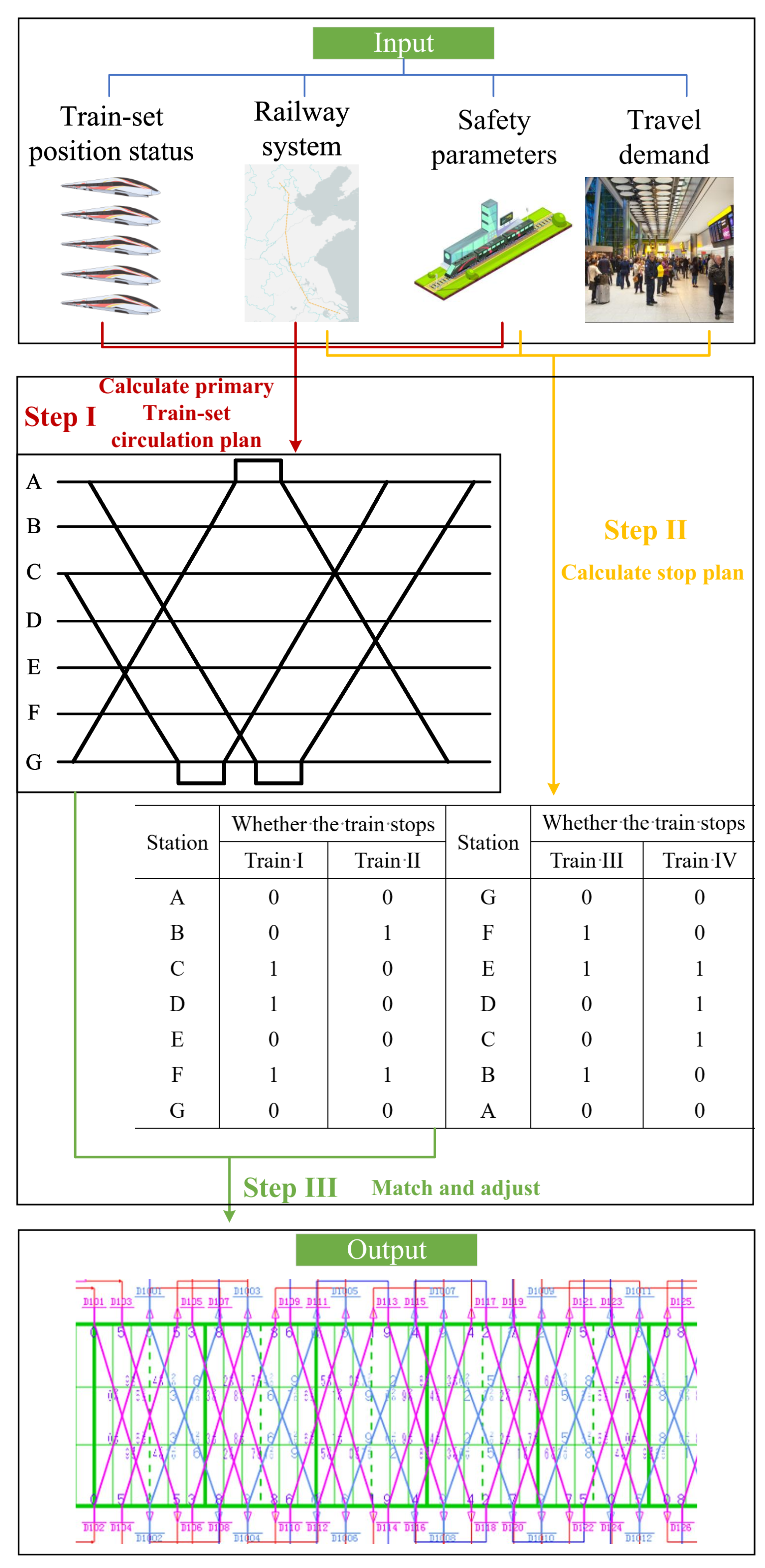
In the normal approach, a train timetable is scheduled at first, to meet the passenger travel demands. Then the train-set circulation plan is scheduled according to the timetable. The disadvantage is, as mentioned above, that it leads to a waste of resources. Moreover, if the operation department only adjusts the timetable to meet the new state requirements, it will affect the satisfaction of passenger travel demands too. It is very difficult to solve the train timetable and the train-set circulation plan directly at the same time because the scale of the problem is too huge for long distance HSR lines and the time consumption will be unacceptable. The approach proposed in this paper aims to meet the demands of passengers as much as possible, without affecting the robustness of the implementation of the new timetable, and avoid the waste of resources. We calculated the train-set circulation plan and stop plan respectively, and finally matched them to obtain the timetable. The scale of each problem is smaller than the overall problem, which is easy to solve. The approach framework used in this paper is shown in Figure 4.

As shown in Figure 4, we need the structure of the HSR, the operation safety parameters of the HSR, the position of the train-sets in the new state and the old state, and the travel demand of passengers before scheduling the transition timetable and the train-set circulation plan.

The first step is to calculate the primary train-set circulation plan according to the position and state data of the train-set, the structure of the HSR and the operation safety parameters. We established a profit function according to the full load ratio of trains in different sections. The higher the load rate of the train, the higher the profit. Based on the profit function, we build an integer programming model with profit maximization as the goal and use CPLEX to solve. The plan obtained in this step is called the primary train-set circulation plan, which will be used in the third step to match with the stop plan.

The second step is to calculate the stop plan according to the structure of HSR, operation safety parameters and passenger travel demands. The calculation of the stop plan should be based on the service plan. If a train arrives, departs, or passes through a station, we call the train serves the station. In the service plan, we define the minimum quantity of trains that stop at each station. Moreover, the quantity of trains is calculated by decomposing the passenger travel demands. The stopping plan here is used to match the train-sets of the primary train-set circulation plan.

The third step is to match the primary train-set circulation plan and stop plan, based on a genetic algorithm (GA). In order to save time, we calculate the train timetable according to the operation safety parameters after the matching scheme is obtained by the GA. We adjust the operation lines beyond the operating time range, to output the final timetable and the train-set circulation plan that meets the operational requirements.

The main contributions of this paper to the study of the TRP and the TTP are as follows:

•  An integer programming model based on profit function was designed, and CPLEX was used to solve the primary train-set circulation plan in a very short time.
•  Based on the decomposition method of passenger travel demands, the service plan is constructed. We use CPLEX to solve the model and obtain the stop plan.
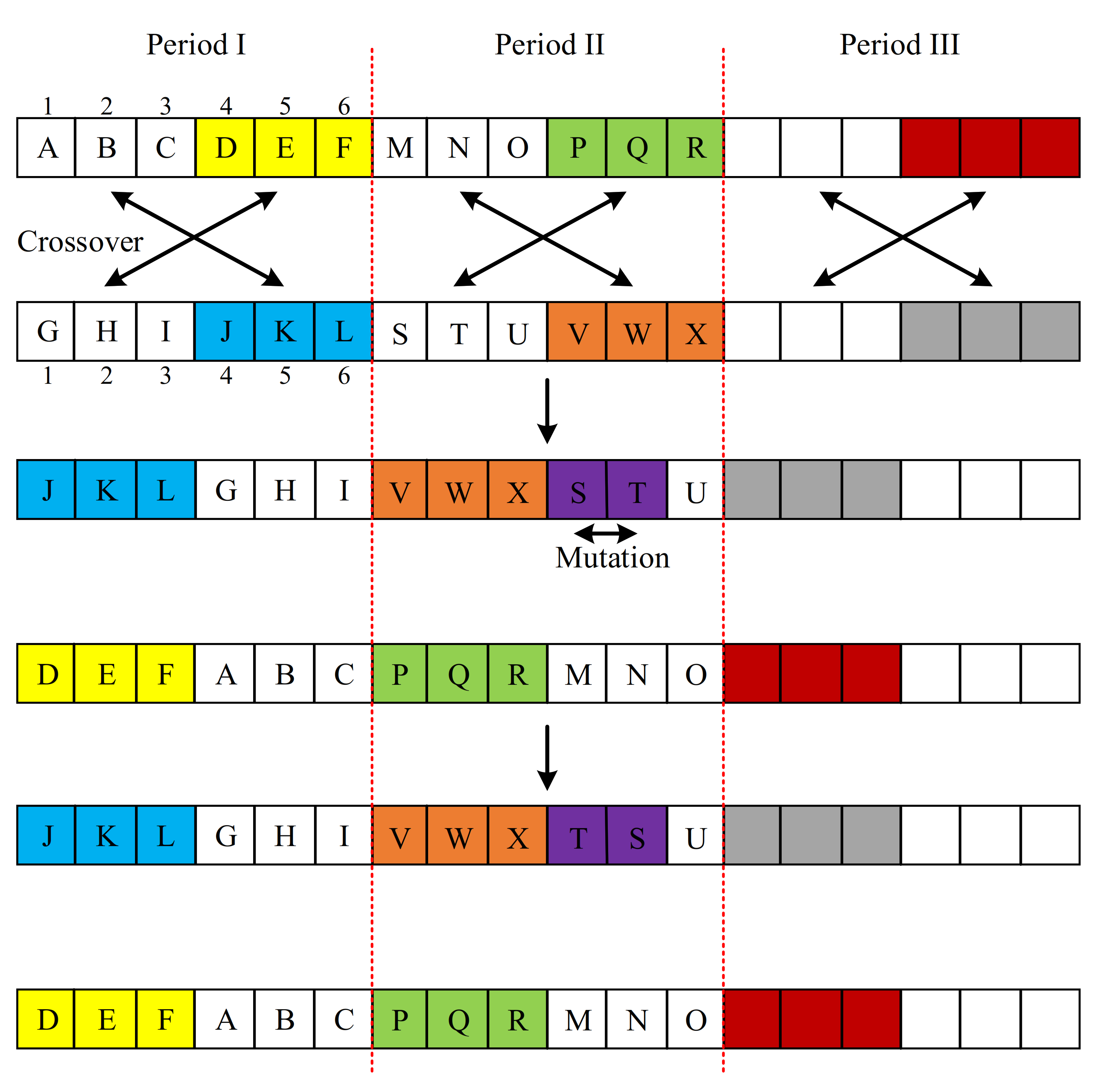
•  We proposed a GA to calculate the matching relationship of the primary train-set circulation plan and the stop plan, then calculate and adjust the timetable according to the safety operating requirements.

The rest of the paper is as follows: In the second section, we summarize the existing research. In the third section, we describe the construction method of the train-set section sequence and the profit function of it and establish the integer programming model for scheduling the primary train-set circulation plan. In the fourth section, we describe the decomposition method of passenger travel demands, which can convert the complex passenger travel demands into a service plan. Then, we introduce a method to calculate the stop plan based on the service plan. In the fifth section, we propose a GA to match the primary train-set circulation plan and the stop plan. Moreover, we design an adjusting method of the plan and timetable, to make them meet the operating requirements. In the sixth section, we carry out a real-world case study on the Beijing-Shanghai HSR. We analyzed the performance of the approach from the perspective of the application. In the seventh section, we summarize the paper and present the recommendations for further research.

2. Literature Review

2.1. Train-Set Rescheduling Problem

There are two scenarios of TRP. The first scenario is to optimize the train-set circulation plan corresponding to the current timetable, to meet the demands of the new timetable. Abbink et al. [1] optimized the allocation of locomotives and vehicles and built a model to match the vehicle model with the line demand. They use CPLEX to solve it. The results show that the plan prepared by the algorithm can significantly improve the service quality in the peak period, compared with the manual scheduling plan. Fioole et al. [2] considered the indicators, such as railway operation cost, reliability and service quality when optimizing the railway rolling stock circulation problem. Their model can serve multiple lines and realize train combination and splitting. Their method has been applied to railway lines in the Netherlands. Cacchiani et al. [3] established a model by corresponding train units and a given set of timed trips for solving the train-unit assignment problem (TUAP). Moreover, they considered the number of seats required by passengers on each trip. Cadarso et al. [4] designed a model including shunting operations, propagated delays and the need for human resources. Through this model, the synchronous arrangement of locomotive and vehicle allocation and vehicle path is realized. They used the heuristic based on Benders Decomposition to solve the model. Lin et al. [5] studied a train-unit scheduling problem (TUSP), which is similar to the TUAP. Compared with TUAP, they took more real-life factors into consideration, which are crucial in railway operation. They proposed a customized branch-and-price solver and adapted an adaptive node selection method to facilitate the solving process.

For the railway system that contains different types of trains, there are different maintenance requirements. Thus, in some application scenarios, the maintenance factors need to be considered when scheduling the train-set circulation plan.

Maróti et al. [6] proposed a train timetable adjusting the approach for trains that require maintenance within three days. Alfieri et al. [7] studied the efficient cycle of rolling stock. They established an integer multicommodity flow model to maximize the use of vehicles. They consider coupling trains in peak hours. Peeters et al. [8] put forward a method to adjust the number of trains at stations along the railway line by branch pricing algorithm. Chung et al. [9] proposed a mixed integer programming model of balance train route mileage. This model considers the limitation of maintenance capacity. Budai et al. [10] proposed a method to reschedule the train-set circulation plan based on a current timetable, so as to meet the demands of the new timetable. Otsuki et al. [11] described the railway rolling stock allocation problem based on a set partitioning multi-commodity flow (SPMCF) problem. Thorlacius et al. [12] constructed the rolling stock plan by using a heuristic algorithm. For specific needs, they use a hill climbing heuristic to optimize the obtained plan, to maximize the carrying capacity with as few trains as possible. Lai et al. [13] established a model to improve the efficient utilization of rolling stock. They considered the overhaul of the train. The case study shows that their method can improve train-set utilized efficiency and solution efficiency. Zhou et al. [14] compare the TCPP to the aircraft route problem (ARP) and the vehicle route problem (VRP) in logistics. They proposed a train-set circulation optimization model, an effective multiple population genetic algorithm (MPGA) is used to solve the problem. Aims to minimize the cost of rescheduling train-sets, Nishi et al. [15] described the TCPP as a traveling salesman problem (TSP) and then solved it by a column generation and Lagrangian relaxation heuristics. Wang et al. [16] studied the train utilization of railway transportation hubs. They built a TCP model. In this model, there is a one-to-one responsibility relationship for train-sets, trip tasks, and maintenance. They designed a genetic algorithm to solve it. A case study shows that dispatching trains between stations in the hub can improve efficiency.

The second scenario of TCPP is that if there are emergencies in railway operation, how to reschedule train-sets after the emergency. It is also called the rolling stock rescheduling problem (RSRP), which is similar in feature to the TCPP. Rezanova et al. [17]. studied the train driver recovery problem (TRDP), which is similar to the RSRP. They treat TDRP as a set partitioning problem and adopt a depth first search of the branch & bound tree to obtain integer solutions. They tested the method based on data from the Danish passenger railway. Nielsen et al. [18] proposed a rolling stock management approach for the case of disturbed operations. The rolling stock decision is considered only for a period of time. After arranging the trains during the current period, the next period will be considered. Through this rolling horizon approach, they improve the solution efficiency. From the perspective of passenger service, Ilse et al. [19] proposed an integer programming model to determine which trains still operate after being disturbed. They tested the method on the Dutch railway. Wagenaar et al. [20] proposed a mixed integer linear programming rescheduling model including passenger demands. It is also suitable for train rescheduling problems with sudden changes in passenger demands. Ghaemi et al. [21] studied a mixed integer linear program model suitable for a busy corridor of the Dutch railway to obtain the short-turn scheme under disruption. The results show that the short-turn scheme is related to the disruption length and longer disruption length will cause more train cancellations. The research on the first scenario focused on rescheduling the train-set circulation plan under the existing timetable. Moreover, the research on the second scenario focused on adjusting the train-set circulation plan and timetable at the same time. The new timetable is different from the old timetable; therefore, the ideal train-set circulation plan corresponding to the two is also different. There are limitations in meeting the train-set demands of the new timetable by optimizing the train-set circulation plan on the old timetable. We refer to the idea in the second scenario to schedule a timetable and train-set circulation plan at the same time on the premise of meeting the needs of passengers.

2.2. Train Timetabling Problem

TTP includes periodic timetabling, aperiodic timetabling, and mixed timetabling. Mixed timetabling is a combination of periodic timetabling and aperiodic timetabling.

Many researchers use the periodic event scheduling problem (PESP) model to study the periodic TTP. In 1996, Odijk et al. [22] proposed that different types of trains can have different operation cycles. According to different types of trains, the operation line of each type of train shall schedule the timetable according to their respective cycles. The model stipulates that each type of train has the same starting and ending points, train routes, stop plans. Kroon et al. [23] found that the train running time is fixed in some models but in the actual situation they are unfixed. Thus, they estimated that the train running time is unfixed and then designed a model based on the PESP model. Jamili et al. [24] proposed a hybrid multivariable hydraulic algorithm to solve the PESP model. In the model, multiple kinds of trains are operated on a single-track railway. Siebert et al. [25] studied the periodic timetabling problem models actually applied in the Netherlands railways and the Berlin subway. They additionally considered passenger paths and line frequencies and then verified the model on the railway in Germany. A case study showed that the travel time of passengers is shorter in the extended model. Based on their previous studies, Kroon et al. [26] further studied the periodic train timetable’s intersection and transfer connection. Heydar et al. [27] describe the method of applying the PESP to the existing periodic timetable scheduling problem, the shortcomings of the existing models are analyzed, and an extended model allowing partial deviation of the running time is proposed. Lamorgese et al. [28] divide the railway line into a series of independent units. They established a decision-making model for the time and priority of the train. Zhou et al. [29] established a model for scheduling timetables for different types of trains. In this model, the operation line of each train is scheduled according to its own period. Each type of train has the same starting and ending points, train path, stop plan and speed. Sparing et al. [30] established a cycle timetable optimization model for pursuing the minimum cycle time. They believe that a short cycle length can make the timetable more stable. Burggraeve et al [31]. proposed a method of scheduling a robust timetable. They first generate a line plan, then schedule a timetable based on the line plan by PESP model, and feedback the quality of the line plan with the buffer time of the timetable. The variable time length of the critical line makes the method more flexible. They verified the algorithm with the railway network structure of Copenhagen, and the results show that robustness can be improved. Zhang et al. [32] transformed the mathematical model of PESP into a multi commodity network flow model with two coupled schedule networks and sidetrack capacity constraints. Through this model, they synchronize limited operational resources toward a master periodic schedule of transport services.

In terms of aperiodic timetable, Ghoseiri et al. [33] proposed a multi-objective model, in which fuel consumption cost is adapted to evaluate the operation department’s satisfaction. Doflman et al. [34] proposed the discrete event model of trains to dispatch trains in the railway network. In this model, they adopted the local feedback-based travel advance strategy to deal with the disturbances in the timetable. Considering that both the section capacity and the station capacity are limited resources, Zhou et al. [35] add a set of operational constraints. The branch and bound algorithm and the Lagrangian relaxation algorithm are adapted to calculate the train timetable. Cacchiani et al. [36] put forward a model in which all variables are related to the train running time. They solved the model using heuristic and exact algorithms. This method is not suitable for large-scale railway networks. They proved the effectiveness of the algorithm through some small-scale examples. Lee y et al. [37] used the heuristic method of optimization to generate the initial solution and then iterated. They used two systems, one to determine the sequence of trains passing through the station and the other to calculate the timetable. They verified the effectiveness of the understanding on two small-scale road networks. Forsgren et al. [38] developed a model based on Sweden’s new timetable scheduling process to meet the transportation demand when the infrastructure capacity changes. Sun et al. [39] established a multi-objective optimization model. In this model, they set a series of objectives including the average train running time, energy consumption and passenger satisfaction. To solve the problem, they designed an improved genetic algorithm. Shi et al. [40] analyzed the train operation plan optimization problem of an urban rail corridor. The railway system is divided into two parts: platform and vehicle. They aim to minimize the number of train departures, so as to meet the needs of passengers while driving as few trains as possible. Tong et al. [41] proposed a space-time network that is based on three dimensions. Then they calculated the train timetable by a train timetable compilation method. Jiang et al. [42] established a DEA model based on train routes, so as to provide a basis for train route selection. Fischer et al. [43] studied aperiodic TTP. They found that linear programming could not describe the overtaking relationship of trains. Therefore, the problem was decomposed into several subproblems by the connected configurations method, and Lagrange relaxation was used to solve these subproblems. Wang et al. [44] proposed a column generation algorithm with an acceleration scheme to solve the train timetable. Wang et al. [45] proposed a space-time decompose approach to analyze the passenger travel demands. They established an integer programming model, which divides the timetable into three periods and solves the corresponding timetable in parallel.

In terms of periodic and aperiodic mixing TTP, [28,46,47] studied the problem from the perspective of maximizing the profit of the operating company and the perspective of passengers’ satisfaction.

A periodic timetable is easier to solve, but in periodic timetables, some trains with excessive stops are repeated to meet the travel demands of passengers. This kind of train will lead to low passenger satisfaction. Due to the difficulty of solving aperiodic timetables directly, the time consumption will be beyond acceptance. Although the solving speed of periodic and aperiodic mixing timetable is faster, it is still a timetabling priority method, which may not be optimal for the train-set circulation plan. Moreover, there is some research on timetable rescheduling under disruptions; [48,49,50,51] studied the timetable rescheduling problem with different strategies. They adjust the train stop plan and operating order to erase the negative effect as soon as possible.

Most of the existing research deals with traditional TRP and TTP. Those studies are suitable for traditional operation scenarios, but transition time is a distinct scenario. Moreover, some research connected with TTP, on rolling stock rescheduling, is for the disturbed scenarios. The goal of these scenarios is to resume normal operation as soon as possible. Although there are some studies on transition time, the problem of wasting resources when timetable adjusting frequency increases still cannot be solved because much of the research is based on the current timetable. Hence, we propose a specific approach to TRP and TTP for transition time, in which the train-set circulation plan has a priority, to avoid the problems mentioned above.

3. Primary Train-Set Circulation Plan

The long distance HSR line has more stations, and there are more train-sets running on it. Thus, it is more complex to decide in which direction the train-set will be operated and how long should the train-set run. We proposed an integer programming model to obtain the primary train-set circulation plan. The objective of the model is to maximize the profit of train-set operation under the premise of meeting the train-set position constraints. The profit function is constructed based on the full load ratio associated with time.

3.1. Notations

Table 1. General subscripts.

Subscripts	Description
$i$	Train-set $i\in I$,where $I$ is the set of train-sets, $\left|I\right|=n$.
$j$	Section $j\in J$, where $J$ is the set of sections, $\left|J\right|=m$.

lists the general subscripts of the proposed model. Moreover,

Table 2. Description of the parameters.

Subscripts	Description
$P_j^i$	The profit of train-set $i$ when train-set $i$ passing section $j$.
$C^i$	The capacity of train-set $i$.
$C_j$	The total capacity of all train-sets in section $j$.
$D_i$	The depart time of train-set $i$.
$E_j$	The ticket price of section $j$.
$Q_j$	The quantity of passengers in section $j$.
$F_j$	The average full load ratio of section $j$.
$S_j^i$	Whether train-set $i$ passing section $j$.
$T_s$	The starting time of the operation hours.
$T_e$	The end time of the operation hours.
$T_j^i$	The running time of train-set $i$ in section $j$.
$T_d$	The departure interval
$u_i$	Whether train-set $i$ goes in the direction $u$.
$d_i$	Whether train-set $i$ goes in the direction $d$.
$N_j$	Number of train-sets required by the station at the end of the section $j$ in the new state.
$S_u^i$	The starting section of train-set $i$ for the direction $u$.
$S_d^i$	The starting section of train-set $i$ for the direction $d$.

lists the parameters used in the proposed model.

3.2. Profit Function

The operating profit of the train-set is related to the full load ratio. The full load ratio of section $j$ can be calculated as:

$$F_j=\frac{Q_j}{C_j}$$

(3)

where $Q_j$ means the quantity of passengers of section $j$, and $C_j$ means the sum of the capacity of all train-sets of section $j$. The full load ratio of a section can be calculated on the basis of historical passenger transport data.

The passenger travel demands of different sections and times are different. Therefore, the full load ratio of the train-sets operating in these sections will also be different. By comparing the full load ratio of train-sets, we can observe the passenger demands in this section. At the same time, the full load ratio of the train-set directly reflects the profits of the train-set. The high load ratio of the train-set shows that it has a high income. More train-sets are needed for the sections with high travel demand for passengers. For the section with less travel demand, train-sets can be operated less appropriately. Therefore, the profits of train-set operation come from the quantity of passengers.

In this paper, we evaluate the profits based on the full load ratio of train-sets in the section. It represents the profits generated by a train-set passing through a section. This benefit is used as a reference when calculating the stop position of the train-set under the condition of satisfying the state constraint at the end of the transition time. The profit is related to the train-set operating direction. The train-set operating direction of stations at both ends of the HSR line is fixed. Moreover, there are two directions for train-sets at intermediate stations. Figure 5 shows the train-set direction of the stations at both ends and the train-set direction of the intermediate station.

As shown in Figure 5, train-set 1 can only perform the operation line in the A-G direction at station A, like the blue line. The same train-set 3 can only perform the G-A direction at G station, like the red line. There are two options for train-set 2 departing from station C. One is to perform the C-A direction, like the green line. Moreover, the other is to perform the direction of C-G, like the yellow line.

Thus, we sum the profit of each section to evaluate the operating profit. The profit function $P\left(i\right)$ for train-set $i$ is as follows:

$$P\left(i\right)={\displaystyle \sum }_j\left(P_j^i\times S_j^i\right)$$

(4)

where $S_j^i$ means that whether train-set $i$ passing section $j$, $P_j^i$ means the profit of train-set $i$ pass through section $j$. Let $F_j$ be the full load ratio of section, $j$, $C^i$ be the maximum quantity of passengers that can be carried by train-set $i$, which is called the capacity of train-set $i$, $E_j$ be the ticket price of section $j$, we can rewrite the profit function $P\left(i\right)$ as:

$$P\left(i\right)={\displaystyle \sum }_j\left(P_j^i\times S_j^i\right)={\displaystyle \sum }_j\left(F_j\times C^i\times E_j\times S_j^i\right)$$

(5)

3.3. Section Division

In HSR operation, stations are divided into different grades. Stations of different grades have different operational capabilities. Only high-grade stations are qualified to be the starting station and terminal station of train-sets. We regard these stations as the boundary stations of the section. Figure 6 shows an example of sections and boundary stations.

As shown in Figure 6, stations A, C, E and G are boundary stations, and stations B, D and F are ordinary stations. In this model, we divided these stations into three sections, they are section A-C, section C-E and section E-G. Train-sets are only allowed to end their operation at stations A, C, E and G. Each section has a start station and an end station. For example, for section A-C, the start station is station A, and the end station is station C. It should be noted that there may not be only one station in the middle of the boundary section.

3.4. Train-Set Section Sequence

In this paper, we construct a train-set section sequence based on the running direction of the train-set. The sequence can reflect the direction and route of the train-set. The longer the one-way travel distance of the train, the more diverse passenger travel demands can be borne. Therefore, we default that all trains will run as long as possible once they are operated, to meet more travel demands of passengers. The train-set direction sequence is shown in Figure 7.

As we can see in Figure 7, stations A, C, E and G are boundary stations. Train-set 1 at station A has only one direction. In Figure 7a, train-set1 perform the blue line, and the corresponding train-set direction sequence is shown as the blue route in Figure 7b:

A-C, C-E, E-G, G-E, E-C

Similarly, train-set 3 at station G has only one direction, and its train-set section sequence is shown as the red route in (b), which is:

A-C, C-E, E-G, G-E, E-C

G-E, E-C, C-A, A-C, C-E

Train-set 2 at station C has two directions, either to station A or G. These two directions correspond to a different sequence of the route. In this case, we add the routes corresponding to the two directions to the train-set section sequence in the model. The sequence of train-set 2 is:

(1)C-E, E-G, G-E, E-C, C-A

(2)C-A, A-C, C-E, E-G, G-E

3.5. Objective Function and Constraints

3.5.1. Objective Function

$$\mathit{max}{\displaystyle \sum }_{i=1}^{n}P\left(i\right)$$

(6)

We designed an objective function for maximizing the operating profits of all the train-sets. It aims to meet more demands of passengers.

3.5.2. Constraints on Operation Time

$$T_s\le D_i\le T_e$$

(7)

$D_i$ means the departure time of the train-set $i$ in its starting station, $T_s$ means the start time of operation hours, $T_e$ means the end time of operation hours. HSR has a fixed operation hour, and the train-set’s departure time and arrival time need to meet the operating time range. In addition, we stipulate that the end operation time of the train-set should be within the operating time range.

$$D_i+{\displaystyle \sum }_{j=1}^n\left(R_j^i\times S_i^i\right)\le T_e$$

(8)

$R_j^i$ means the running time train-set $i$ in section $j$. When setting the running time, we set aside redundancy because the dwell time of train-sets at stations within the section and the turn-back time also needs to be considered.

3.5.3. Constraints on Departure Interval

$$D_{i+1}-D_i\ge T_d$$

(9)

Based on the safety operation requirements of railway transportation, the adjacent train-sets should maintain a safety interval. $D_{i+1}$ means the departure time of the train-set, $T_d$ means the departure interval of the train-set.

3.5.4. Constraints on Direction Selection

$$u_i+d_i=1$$

(10)

Train-sets in the intermediate station need to choose the direction based on the profits, and only one direction can be selected. $u_i$ means the train-set $i$ chooses the $u$ direction, $d_i$ means the train-set $i$ chooses the $d$ direction. $u_i$ and $d_i$ are 0-1 variables. 0 means that the direction is not selected, and 1 means that the direction is selected. The sum of $u_i$ and $d_i$ is 1 to ensure that only one of the two directions can be chosen.

3.5.5. Constraints on Matching of Direction and Section Sequence

$$\left\{\begin{array}{c}{u}_i=S_u^i\\ d_i=S_d^i\end{array}\right.$$

(11)

The section sequence covers the sequence corresponding to two directions. $S_u^i$ means the starting section of the sequence in the $u$ direction, $S_d^i$ is the starting section of the sequence in the $d$ direction.

3.5.6. Constraints on Section Sequence

$$S_j^i\ge S_{j+1}^i$$

(12)

$S_j^i$ is 0-1 variable. 0 means the train-set $i$ does not pass through the section $j$, 1 means the train-set $i$ passes through the section $j$. The section sequence represents the route of the train-set. The constraint on the section sequence is to ensure the continuity of train-set operation and avoid the phenomenon of occupying section $j$ and $j+2$, skipping section $j+1$.

3.5.7. Constraints on Final Position of Train-Set

$${\displaystyle \sum }_{i=1}^n\left(S_j^i-S_{j+1}^i\right)=N_j$$

(13)

$N_j$ means the number of train-sets required by the station in the new state. The station here refers to the boundary station at the end of section $j$. After the operation of the transition time, the position of the train-set shall meet the final position constraints, which are also the position requirements of the train-set at the beginning of the new state. We represent the stop position of the train-set by the occupation of adjacent sections. As mentioned above, $S_j^i$ means that whether the train-set $i$ passes through the section $j$. If the train $i$ passes through both section $j$ and section $j+1$, then there will be $S_j^i=1$, $S_{j+1}^i=1$ and $S_j^i-S_{j+1}^i=0$. It indicates that the train-set $i$ does not stop at the end station of section $j$. Conversely, if the train-set $i$ passes through the section $j$ but does not pass through the section $j+1$, then $S_j^i=1$, $S_{j+1}^i=0$, $S_j^i-S_{j+1}^i=1$. It means that the train-set $i$ stops at the end station of section $j$.

4. The Passenger Travel Demand Decomposition and Stop Plan

4.1. Problem Description

In the previous section, we got a primary train-set circulation plan. The plan is section-specific and lacks a specific stop plan for the train-set in each station. To calculate the stop plan, we need to know the service plan first. The service plan includes the number of stops at each station. It is determined according to the travel demands of passengers. We use the passenger demands space-time decomposition method [45] to calculate the service plan. The space decomposition result is used to calculate the quantity of stops in each station, and the time decomposition result will be used in Section 5 to evaluate the match relationship of stop plan and primary train-set circulation plan. Based on the service plan, the stop plan is calculated by CPLEX. In order to save operating costs, we take minimizing the number of stop schemes as the objective function. The passenger travel demands in each direction are different, and the stop plan corresponding to the direction is also different. Thus, we calculate the stop plan for different directions separately. The calculation of the stop plan is similar in each direction. Therefore, we mainly discuss the stop plan calculation in one direction.

4.2. Notations

Table 3. General subscripts.

Subscripts	Description
$k$	Station $k\in K$, where $K$ is the set of stations, $\left|K\right|=a$.
$l$	Type $l\in L$, where $L$ is the set of stop plan types, $\left|L\right|=b$.

is the description of general subscrips of the approach we used in this paper, and

Table 4. Description of the parameters.

Subscripts	Description
$S_k$	The minimum quantity of train service at station $k$.
$Q_k$	The number of passengers that station $k$ served in one day.
$Q^L$	The number of passengers on the railway line that we are concerned about.
$Q^T$	The total amount of passengers served on all the railway lines passing through station $k$ in one day.
$C$	The average capacity of a train.
$O^{l,z}$	Whether the $z-th$ scheme in type $l$ is operated.
$V_k^{l,z}$	Whether the $z-th$ scheme in type $l$ stops at station $k$.
$V^l$	The maximum number of stops of scheme in type $l$.
$V_k$	The minimum number of train service at station $k$.
$U^l$	The maximum number of schemes of type $l$.

is the description of the parameters in the approach.

4.3. Passenger Travel Demand Decomposed

If a train departs, arrives, or passes through a station, we call the train serves the station. The service plan defines the minimum quantity of train service at each station.

For stations at both ends of the railway, we use the following method to calculate $S_k$, the minimum quantity of train-set service:

$$S_k=\frac{Q_k}{C}$$

(14)

where $Q_k$ means the number of passengers that station $k$ served in one day. $C$ means the average capacity of a train. In this paper we default that all the train-set has the same capacity, hence $C$ is equal to the capacity of a single train-set.

Considering that the train-set has carried passengers before it arrives at the intermediate station, we need to consider the average full load ratio between adjacent stations of a section when calculating the quantity of train service for the intermediate station. It should be noted that the section here is different from Section 3.3. Section 3.3 is for boundary stations, and the section here is for adjacent stations. The corresponding relationship of the full load ratio and the station is shown in Figure 8.

As shown in Figure 8, $F_{A-B}$ is the average of section A-B, hence the number of passengers train-set can transport in station B can be written as:

$$C_B=C\times \left(1-F_{A-B}\right)$$

(15)

Therefore, we use the following method to calculate the minimum quantity of train service for an intermediate station $k$ in section $j$:

$$S_k=\frac{Q_k}{C_k}=\frac{Q_k}{C\times \left(1-F_k\right)}$$

(16)

$F_k$ means the average full load ratio of a train at section $k$, which is connected with station $k$. The full load ratio of trains is different in different directions at the same station.

There are some stations that serve several railway lines, which are called hub stations. For these stations, the calculation method for the minimum quantity of train-sets has two types similarly. For hub stations at both ends of the railway, we write the formula as:

$$S_k=\frac{Q_k\times \frac{Q^L}{Q^T}}{C}$$

(17)

And for other hub stations, we write the formula as:

$$S_k=\frac{Q_k\times \frac{Q^L}{Q^T}}{C\times \left(1-F_k\right)}$$

(18)

$Q^T$ means the total amount of passengers served on all the railway lines passing through station $k$ in one day. $Q^L$ means the number of passengers on the railway line we are concerned about.

4.4. Type of Scheme in Stop Plan

As mentioned above, the operation line in the timetable is a task for train-set. It corresponds to a scheme in the stop plan. An operation line needs to be implanted by a train-set.

Table 5. An example of stop plan.

Station	Whether Train-Set Stop				Station	Whether Train-Set Stop
	S I	S II	S III	S IV		S V	S VI	S VII
A	1	1	-	1	G	1	1	1
B	0	0	-	0	F	1	0	0
C	1	0	1	0	E	0	1	1
D	0	1	0	1	D	1	0	-
E	1	1	0	0	C	0	0	-
F	0	0	1	0	B	0	1	-
G	1	1	1	1	A	1	1	-

shows an example of a stop plan.

There are seven schemes in the stop plan. Schemes in the stop plan can be divided into different types according to their departure station and terminal station. Thus, there are four types of schemes, scheme I, II, IV are the first type, scheme III is the second type, schemes V, VI are the third type, scheme VII is the fourth type. The service distance of scheme I is from station A to station G, it is longer than scheme III, hence scheme I can serve more diverse passenger travel demands. Thus, schemes with longer service distances have higher priority.

4.5. Objective Function and Constraints

4.5.1. Objective Function

$$\mathit{min}{{\displaystyle \sum }}_l{{\displaystyle \sum }}_z{E}_l^z$$

(19)

$E_l^z$ is a 0-1 variable, which means whether the $z-th$ scheme in type $l$ is operated. Obviously, the operation department can save costs by operating as few schemes as possible under the premise of meeting the passenger travel demands.

4.5.2. Constraints on the Quantity of Train Service

$${\displaystyle \sum }_{l=1}^b{V}_k^{l,z}=V_k$$

(20)

$V_k^{l,z}$ is a 0-1 variable, indicating whether the $z-th$ scheme in type $l$ serves station $k$. $V_k$ is the number of services required by the station $k$.

4.5.3. Constraints on the Maximum Number of Stops

$${\displaystyle \sum }_{k=1}^a{V}_k^{l,z}=V^l$$

(21)

If the scheme $l$ stops too many times, the running time will be too long. It will affect the travel efficiency of passengers. Moreover, the negative impact will be amplified especially on long-distance railway lines. A much longer time is needed for the train to complete the journey. Thus, we limit the maximum number of stops of a train. $V^l$ is the maximum number of stops of type $l$.

4.5.4. Constraints on Whether Operating the Scheme

$$V_k^{l,z}\le O^{l,z}$$

(22)

We define that if a scheme is not operated, it should not serve any station. $O^{l,z}$ is a 0-1 variable, $O^{l,z}=0$ means that the $z-th$ scheme of type $l$ has not been operated, and $O^{l,z}=1$ means that the $z-th$ scheme of type $l$ is operated.

4.5.5. Constraints on Scheme Type

$${\displaystyle \sum }_z{O}^{l,z}\le U^l$$

(23)

We define the maximum number of schemes for each type, in order to reduce the calculation scale and conform to reality because the number of trains that can be operated in a day is limited.

5. Timetable Calculation and Adjustment

After the stop plan is obtained, we need to match the primary train-set circulation plan and the stop plan, to obtain the final train-set circulation plan and transition timetable. The flow chart of the timetable calculation and adjustment method is shown in Figure 9. Green is the input part; Blue is the matching part and Orange is the adjustment part. The operation of each step will be described in detail below.

5.1. Primary Train-Set Circulation Plan Splitting and Corresponding Relationship

To match the primary train-set circulation plan, firstly we need to split the primary train-set circulation plan. The schematic diagram of the method for splitting and matching is shown in Figure 10.

In Figure 10, the route of train-set I contains three schemes ➀, ➁ and ➂. The route of train-set II contains four schemes ➃, ➄, ➅ and ➆. Scheme ➀, ➂ and ➅ are from station A to station G, and they can be matched with scheme I, II and IV in stop plan. Scheme ➁ and ➄ are from station G to station A, and they can be matched with scheme V and VI. There are triangle areas in the timetable, like purple triangles and green triangles. The triangle area is the area between the trains that depart from the stations at both ends and the starting time of the operation hours. The green triangles are for direction A-G, and the purple triangles are for direction G-A. The Triangle area can be served by trains departing from intermediate stations. Thus, scheme ➃ can be matched with scheme III, and scheme ➆ can be matched with scheme VII.

Figure 10. The schematic diagram of the method for splitting and matching.

Figure 10. The schematic diagram of the method for splitting and matching.

5.2. The Matching Method

5.2.1. The Interconnection Relationship

There is a complex interconnection relationship between trains. The interconnection relationship is shown schematically in Figure 11.

In the example, if train ➀, ➁ and ➂ follow the order on the left, the operation time needed is $T_{ALL}^1$, and if they follow the order on the right, the operation time needed is $T_{ALL}^2$. Obviously, the $T_{ALL}^2$ is shorter than $T_{ALL}^1$, hence the efficiency is higher on the right. When matching the primary train-set circulation plan with the stop plan, we need to consider the interconnection relationship of trains, i.e., the order of trains.

Figure 11. The schematic diagram of the interconnection relationship.

Figure 11. The schematic diagram of the interconnection relationship.

5.2.2. Matching and Adjusting Method

When matching the stop plan with the primary train-set circulation plan, something needs to be considered. First, the number of schemes in the primary train-set circulation plan may be different from the number of schemes in the stop plan. Second, although we have reserved the stop time when calculating the primary train-set circulation plan, it is still possible for the train to exceed the prescribed operation hours when it ends operation. In order to ensure that the timetable meets the actual requirements, we design a matching and adjusting method for the above situations, as shown in Figure 12.

As shown in Figure 12, the matching and adjusting method of the stop plan and the primary train-set circulation plan are divided into three parts.

•  Firstly, we compare the number of schemes in the stop plan with the number of schemes in the primary train-set circulation plan and take these data as input data. In the matching process, we adjust the scheme according to the comparison results. If the number of schemes in the stop plan is more than the number of schemes in the primary train-set circulation plan, the number of schemes in the stop plan will be reduced. We follow the principle of meeting the travel demands of passengers to the greatest extent and give priority to canceling the scheme with fewer stops. If the number of schemes in the stop plan is less than the number of schemes in the primary train-set circulation plan, it indicates that the carrying capacity of the primary train-set circulation plan is greater than the travel demands of passengers. In this case, we generate the stop scheme for these schemes in the primary train-set circulation plan. These extra schemes in the stop plan only serve boundary stations, because these stations serve more passengers. If the number of trains in the stop plan is the same as the number of schemes in the primary train-set circulation plan, then go to the next step directly.
•  The timetable can be calculated after the number of schemes in the stop plan is equal to the number of schemes in the primary train-set circulation plan. When calculating the timetable, the matching relationship between the stop plan and the schemes of the primary train-set circulation plan should be determined first.

There are differences in the travel demands of passengers at different periods within a day. To meet the travel demands of passengers more accurately, we divide a day into serval periods, and decompose the passenger travel demands in the time dimension, based on the result of space decomposition result. It is a reference to evaluate the matching result because it can show whether the timetable meets the passenger travel demands, which is very important in HSR operation. We have obtained the space decomposition result in Section 4.3, and the $S_k$ can be divided as:

$$S_k^{\left(x\right)}=\frac{Q_k^{\left(x\right)}}{Q_k}\times S_k$$

(24)

where $S_k^{\left(x\right)}$ means the number of stops of station $k$ in $x-th$ period of a day, $Q_k^{\left(x\right)}$ means the number of passengers served by station $k$ in $x-th$ period.

After that, we calculate the matching relationship by GA. GA is widely used in the research in TRP and TTP, like literature [14,16,39], and the results show that the GA has good performance. We take the matching relationship of the primary train-set circulation plan and stop plan as a gene fragment. The GA steps are as follows:

Step 1. Initial feasible solutions for the matching relationship, and decompose the passenger travel demands.

Step 2. Calculate the timetable for each solution by CPLEX according to the safety operation constraints in real life.

Step 3. Crossover operation. We take a matching relationship as a gene. A multi-point crossover method is used in the algorithm. We cross over the matching relationship based on the periods of time, and the probability of cross over is 0.9.

Step 4. Mutation operation. The mutation operation is to exchange two adjacent matching relationships. The probability of the mutation operation is 0.1. The schematic diagram of crossover operation and mutation operation is shown in Figure 13.

As shown in Figure 13, the schemes of the primary train-set circulation plan are the outer frame. For example, the square numbered 1 represents the first scheme in the primary train-set circulation plan. Moreover, scheme A in the square numbered 1 means that scheme A in the stop plan is matched with the first scheme in the primary train-set circulation plan. Then we perform crossover and mutation operations. Firstly, we divided the matching relationship according to the pre divided time period. All of the operations mentioned above are performed within the time period that the matching relationship belongs. Secondly, we cross over these matching relationships like Figure 13 shows, the latter segment of the second solution is exchanged with the former segment of the first solution, and then the former segment of the first solution is exchanged with the latter segment of the second solution. After the cross over operation, we will judge whether each matching relationship will mutate, and if so, exchange it and its subsequent matching relationship.

Figure 13. The schematic diagram of crossover and mutation.

Figure 13. The schematic diagram of crossover and mutation.

Step 5. Calculate the timetable for new generation by CPLEX according to the safety operation constraints in real life.

Step 6. Evaluate all the solutions. We evaluate those solutions by counting the satisfaction of passenger travel demands within the specified time period and the number of trains exceeding the end of the operation. It should be noted that before comparing those solutions, we need to normalize the satisfaction of passenger travel demands and the number of trains. We use the classical normalization method to divide the current value by the maximum value of this parameter in all solutions Then we choose solutions that have better fitness from all the solutions.

Step 7. If the number of iterations reaches the upper limit, or the best solution meets all the demands, end the algorithm, otherwise go back to step 3.

3.

 After calculating the timetable, it is necessary to check whether all train-sets are within the operating hours. Train-sets that are not within the operating hours need to be adjusted. The adjustment steps are as follows:

Step 1. First, we counted the positions of the train-sets beyond the operating hours when they ended operation.

Step 2. Second, we count the positions of these train-sets at the end of their operating time. It is important to note that train-sets need to be stopped at boundary stations. If the train-set is between two boundary stations at the end of the operating time, we terminate the train-set at the first boundary station it passed.

Step 3. After step 2, the train-set position may not meet the position constraints. We need to rebalance these train-sets. Because the total number of train-sets is fixed, a lack of train-sets at some stations means that there are more train-sets than needed at some other stations. For the extra train-sets in stations where there are more train-sets than needed, we terminate it at the station where train-sets are still needed.

The schematic diagram of each step is shown in Figure 14.

As shown in Figure 14, we can see that three train-sets are out of operation hours. One of these train-sets ends at station A, one at station E, and one at station G. At the end of the operation time, train-set 1 is closest to station C, train-set 2 is closest to station E, and train-set 3 is closest to station E. Thus, after the execution of step 2, We can see that among all the adjusted train-sets, the number of train-set stopped at station A changed from 1 to 0, in station C the number changed from 0 to 1, in station E the number changed from 1 to 2, and in station G the number changed from 1 to 0. Comparing the amount of train-sets at each station in the two states, we can see that stations A and G lack one train-set, while stations C and E have one extra train-set. When replenishing trains for stations A and G, we choose stations as close to them as possible, to minimize the impact on the timetable. That is, in order to meet the requirement for the number of train-sets in station A, we adjust the train-set which finally stops at station C. Similarly, in order to meet the requirement for the number of train-sets in station G, we adjust the train-set which finally stopping at station E.

When we calculate the primary train-set circulation plan, we have set aside the running time for each section. Thus, the adjustment on the timetable here will not influence the timetable too much.

6. Case Study

6.1. Introduction to the Beijing–Shanghai HSR

The real-world data of Beijing-Shanghai HSR was used as an example to analyze the feasibility of the model and algorithm. The Beijing-Shanghai HSR is a HSR line connecting Beijing and Shanghai. It is an important railway line for passenger transportation connecting north and south in China. The diagram of the Beijing–Shanghai HSR line is shown in Figure 15.

The Beijing-Shanghai HSR is 1318 km long and the maximum operational speed of this line is 350 km/h. There are 23 stations along the railway line, including six major hub stations in Beijing, Tianjin, Jinan, Xuzhou, Nanjing and Shanghai. We take these hub stations as a collection of boundary stations.

6.2. Parameters

The safety operation parameters we set in the example are shown in

Table 6. The safety operation parameters.

Parameters	Value
Start addition time	2/min
Stop addition time	3/min
Headway	3/min
Departure interval	4.5/min
Arrival interval	4/min
Dwell time	2/min

. These parameters are used to calculate the timetable. The dwell time is usually two minutes. It should be noted that Beijing Nan Station and Shanghai Hongqiao Station have no dwell time. Because the dwell time is for passengers to get on and off trains, they are generally set up at stations along railway lines. These two stations are stations at both ends of the line and will only be used as starting or terminal stations.

According to the data of the number of passengers served by the station, we use the passenger travel demands decomposition method to calculate the service plan. The service plan of each station is shown in

Table 7. The service plan.

Station	Train Service Quantity
Beijing Nan	157
Langfang	22
Tianjin Nan	51
Cangzhou Xi	32
Dezhou Dong	35
Jinan Xi	128
Taian	32
Qufu Dong	26
Tengzhou Dong	31
Zaozhuang	26
Xuzhou Dong	101
Suzhou Dong	29
Bengbu Nan	34
Dingyuan	21
Chuzhou	38
Nanjing Nan	159
Zhenjiang Nan	24
Danyang Bei	24
Changzhou Bei	27
Wuxi Dong	26
Suzhou Bei	32
Kunshan Nan	17
Shanghai Hongqiao	135

. The old state and new state of each boundary station are shown in

Table 8. The train-set position.

Boundary Station	Old State	New State
Beijing Nan	28	35
Tianjin Nan	17	12
Jinan Xi	15	18
Xuzhou Dong	12	9
Nanjing Nan	25	17
Shanghai-Hongqiao	29	35

.

6.3. Results and Analysis

In the GA, we divided the whole day into three periods. The first is from 6:00 to 12:00, the second is from 12:00 to 18:00, the third is from 18:00 to 24:00. The time-dimension decomposition result is shown in Table 9. We set the maximum number of iterations to 300. The solving time is related to the number of initial solutions. To obtain the relationship between the number of initial solutions, the quality of final solutions and the solving time, we set up 30, 50 and 80 initial feasible solutions respectively, and compared the algorithm performance in these three cases. We choose three representative solutions. The comparison is shown in Figure 16, the iteration diagram is shown in Figure 17, and the specific values for these three cases are shown in Table 10.

Table 9. Time-dimension decomposition result.

Station	Period I	Period II	Period III
Beijing Nan	50	59	48
Langfang	7	8	7
Tianjin Nan	16	19	16
Cangzhou Xi	9	13	10
Dezhou Dong	11	13	11
Jinan Xi	39	48	41
Taian	10	12	10
Qufu Dong	8	10	8
Tengzhou Dong	10	13	8
Zaozhuang	8	10	8
Xuzhou Dong	30	41	31
Suzhou Dong	9	11	9
Bengbu Nan	11	13	10
Dingyuan	7	8	6
Chuzhou	12	14	12
Nanjing Nan	50	60	49
Zhenjiang Nan	8	9	7
Danyang Bei	8	9	7
Changzhou Bei	9	10	8
Wuxi Dong	8	10	8
Suzhou Bei	10	12	10
Kunshan Nan	5	6	5
Shanghai Hongqiao	43	51	41

Table 9. Time-dimension decomposition result.

Station	Period I	Period II	Period III
Beijing Nan	50	59	48
Langfang	7	8	7
Tianjin Nan	16	19	16
Cangzhou Xi	9	13	10
Dezhou Dong	11	13	11
Jinan Xi	39	48	41
Taian	10	12	10
Qufu Dong	8	10	8
Tengzhou Dong	10	13	8
Zaozhuang	8	10	8
Xuzhou Dong	30	41	31
Suzhou Dong	9	11	9
Bengbu Nan	11	13	10
Dingyuan	7	8	6
Chuzhou	12	14	12
Nanjing Nan	50	60	49
Zhenjiang Nan	8	9	7
Danyang Bei	8	9	7
Changzhou Bei	9	10	8
Wuxi Dong	8	10	8
Suzhou Bei	10	12	10
Kunshan Nan	5	6	5
Shanghai Hongqiao	43	51	41

Figure 16. The result comparison of three cases.

Figure 16. The result comparison of three cases.

Figure 17. The iteration diagram.

Figure 17. The iteration diagram.

Table 10. Specific values of 30, 50, 80 initial feasible solutions.

Aspects	Case I	Case II	Case III
Solving time (s)	293	733	3062
Quality	869/1207	1025/1207	1142/1207
Adjustments	10	7	5

Table 10. Specific values of 30, 50, 80 initial feasible solutions.

Aspects	Case I	Case II	Case III
Solving time (s)	293	733	3062
Quality	869/1207	1025/1207	1142/1207
Adjustments	10	7	5

In Figure 17, the best solution among 80 initial feasible solutions is better, because if there are more initial solutions, it is more likely to generate better solutions. We evaluate the quality of the timetable in two ways, one is the satisfaction of the number of stops in each period, the other is the number of adjustments required to make the timetable meet the safety operation constraints. The first way has an impact on the quality of the timetable and the second way has an impact on the train-set circulation. The solving speed is the fastest if we only initial 30 feasible solutions. However, from the perspective of passenger satisfaction, there are 1207 stops in the original service plan. In case III the sum of the number of stops in each period is 1142, which is 31.42% higher than case I. Moreover, the number of adjustments in case III is 50% lower than case I. It means that the timetable and the train-set circulation plan in case III is better than case I. From the perspective of practical application, the HSR operation department can select the number of initial feasible solutions generated according to their demands. If they want to obtain higher quality solutions and do not require to obtain solutions in a short time, they can set more initial feasible solutions.

Moreover, we tested the case of not dividing the time, the result shows that although the number of stops is similar to the approach proposed in this paper, the passenger travel demands satisfaction of each period is very poor.

To verify the performance of the GA, we compared the approach proposed in this paper with the normal approach, in which the timetable is solved by CPLEX at first and then adjust the timetable to meet the train-set position constraints. The time consumption of the normal approach is 38 minutes because the CPLEX needs to solve the stop plan and the timetable at the same time. Moreover, the satisfaction of passenger travel demands is 33.8% lower than the case of 80 solutions. This result is caused by the CPLEX solver arranging all the trains with fewer stops at the front of the timetable. This will lead to unbalanced station stops, too few stops of trains in the early period and too many stops of trains in the later period. Furthermore, to meet the train-set position constraints, 12 trains needed to be dispatched, which will cause extra costs.

7. Conclusions

In this paper, an approach is proposed to solve the problem of scheduling the timetable and train-set circulation plan under the frequency switching scenario of the timetable. This approach considers the travel demands of passengers and the operational requirements of HSR. It can save the cost of railway operation department while realizing the state changing of train-set during the transition time.

Firstly, we design an inter programming model including section sequence for train-set, so that the operating distance can be decided based on each section’s operating profits. We use CPLEX to solve the model in a very short time. By this model, we obtained a maximum benefit oriented primary train-set circulation plan, which will be matched with the stop plan.

Secondly, we design a method for solving the stop plan based on passenger travel demands. For the passenger travel demands, we adopted the travel demands decomposition method to covert the complex passenger travel demands into the service plan. Then we use CPLEX to calculate the stop plan according to the service plan efficiently.

Thirdly, we design the matching and adjusting method of the stop plan and the primary train-set circulation plan. In the method, we split the primary train-set circulation plan into different schemes at first. Then we match the schemes in the stop plan and the schemes in the train-set circulation plan by a customized GA we designed. After one-to-one correspondence is determined between the schemes in the stop plan and schemes in the primary train-set circulation plan, the timetable can be calculated. Finally, the final train-set circulation plan and timetable are obtained.

Fourthly, we test the approach we proposed by the Beijing-Shanghai HSR. The results show that for the aspect of passenger travel demands, the approach proposed in this paper can meet 94.61% of passenger travel demands, and the solving efficiency is higher than the normal approach. What is more, it can save the costs of the operation department.

In the future, we will continue to take the practical application as the guidance to study the collaborative scheduling of timetable and train-set circulation plan:

Firstly, some other algorithms can be used to improve the solving efficiency. We will try to use gradient methods and compare the solving efficiency and the quality of solutions between different algorithms.

Secondly, as there are always some stochastic effects that affect railway traffic, we will optimize the reserve deposit between train intervals to balance the railway traffic efficiency and robustness. Moreover, also, we need to study how to recover normal operation order as soon as possible after disturbance.

Thirdly, we will consider adding the maintenance mileage of the train into the model, which is urgently needed in practical applications. The maintenance of the train may affect the scheduling of the circulation plan of the train-set because, under the existing train-set utilization system, the train-set needs to be checked and repaired at specific locations, which may affect the stop position of the train.

References

1. Abbink, E.; Berg, B.V.D.; Kroon, L.; Salomon, M. Allocation of Railway Rolling Stock for Passenger Trains. Transp. Sci. 2004, 38, 33–41. [Google Scholar] [CrossRef] [Green Version]
2. Fioole, P.J.; Kroon, L.; Maróti, G.; Schrijver, A. A rolling stock circulation model for combining and splitting of passenger trains. Eur. J. Oper. Res. 2006, 174, 1281–1297. [Google Scholar] [CrossRef] [Green Version]
3. Cacchiani, V.; Caprara, A.; Toth, P. A Lagrangian heuristic for a train-unit assignment problem. Discret. Appl. Math. 2013, 161, 1707–1718. [Google Scholar] [CrossRef]
4. Cadarso, L.; Marín, Á. Improving robustness of rolling stock circulations in rapid transit networks. Comput. Oper. Res. 2014, 51, 146–159. [Google Scholar] [CrossRef] [Green Version]
5. Lin, Z.; Kwan, R.S. A branch-and-price approach for solving the train unit scheduling problem. Transp. Res. Part B Methodol. 2016, 94, 97–120. [Google Scholar] [CrossRef]
6. Maroti, G.; Kroon, L. Maintenance Routing for Train Units: The Transition Model. Transp. Sci. 2005, 39, 518–525. [Google Scholar] [CrossRef] [Green Version]
7. Alfieri, A.; Groot, R.; Kroon, L.; Schrijver, A. Efficient Circulation of Railway Rolling Stock. Transp. Sci. 2006, 40, 378–391. [Google Scholar] [CrossRef] [Green Version]
8. Peeters, M.; Kroon, L. Circulation of railway rolling stock: A branch-and-price approach. Comput. Oper. Res. 2008, 35, 538–556. [Google Scholar] [CrossRef] [Green Version]
9. Chung, J.W.; Oh, S.M.; Choi, I. CA hybrid genetic algorithm for train sequencing in the Korean railway. Omega 2009, 37, 555–565. [Google Scholar] [CrossRef]
10. Budai, G.; Maróti, G.; Dekker, R.; Huisman, D.; Kroon, L. Rescheduling in passenger railways: The rolling stock rebalancing problem. J. Sched. 2010, 13, 281–297. [Google Scholar] [CrossRef] [Green Version]
11. Otsuki, T.; Aisu, H.; Tanaka, T. A Search-Based Approach to Railway Rolling Stock Allocation Problems. Discret. Math. Algorithms Appl. 2011, 3, 443–456. [Google Scholar] [CrossRef]
12. Thorlacius, P.; Larsen, J.; Laumanns, M. An integrated rolling stock planning model for the Copenhagen suburban passenger railway. J. Rail Transp. Plan. Manag. 2015, 5, 240–262. [Google Scholar] [CrossRef] [Green Version]
13. Lai, Y.C.; Wang, S.W.; Huang, K.L. Optimized train-set rostering plan for taiwan high-speed rail. IEEE Trans. Autom. Sci. Eng. 2016, 14, 286–298. [Google Scholar] [CrossRef]
14. Zhou, Y.; Zhou, L.; Wang, Y.; Yang, Z.; Wu, J. Application of Multiple-Population Genetic Algorithm in Optimizing the Train-Set Circulation Plan Problem. Complexity 2017, 2017, 1–14. [Google Scholar] [CrossRef] [Green Version]
15. Nishi, T.; Ohno, A.; Inuiguchi, M.; Takahashi, S.; Ueda, K. A Combined column generation and heuristics for railway short-term rolling stock planning with regular inspection constraints. Comput. Oper. Res. 2017, 81, 14–25. [Google Scholar] [CrossRef]
16. Wang, Y.; Zhou, Y.; Yan, X. Optimizing Train-Set Circulation Plan in High-Speed Railway Networks Using Genetic Algorithm. J. Adv. Transp. 2019, 2019, 1–12. [Google Scholar] [CrossRef] [Green Version]
17. Rezanova, N.J.; Ryan, D.M. The train driver recovery problem—A set partitioning based model and solution method. Comput. Oper. Res. 2010, 37, 845–856. [Google Scholar] [CrossRef] [Green Version]
18. Nielsen, L.K.; Kroon, L.; Maróti, G. A rolling horizon approach for disruption management of railway rolling stock. Eur. J. Oper. Res. 2012, 220, 496–509. [Google Scholar] [CrossRef]
19. Louwerse, I.; Huisman, D. Adjusting a railway timetable in case of partial or complete blockades. Eur. J. Oper. Res. 2014, 235, 583–593. [Google Scholar] [CrossRef] [Green Version]
20. Wagenaar, J.; Kroon, L.; Fragkos, I. Rolling stock rescheduling in passenger railway transportation using dead-heading trips and adjusted passenger demand. Transp. Res. Part B Methodol. 2017, 101, 140–161. [Google Scholar] [CrossRef]
21. Ghaemi, N.; Cats, O.; Goverde, R.M. Macroscopic multiple-station short-turning model in case of complete railway blockages. Transp. Res. Part C Emerg. Technol. 2018, 89, 113–132. [Google Scholar] [CrossRef]
22. Odijk, M.A. A constraint generation algorithm for the construction of periodic railway timetables. Transp. Res. Part B Methodol. 1996, 30, 455–464. [Google Scholar] [CrossRef]
23. Kroon, L.G.; Peeters, L.W.P. A Variable Trip Time Model for Cyclic Railway Timetabling. Transp. Sci. 2003, 37, 198–212. [Google Scholar] [CrossRef]
24. Jamili, A.; Shafia, M.; Sadjadi, S.J.; Tavakkoli-Moghaddam, R. Solving a periodic single-track train timetabling problem by an efficient hybrid algorithm. Eng. Appl. Artif. Intell. 2012, 25, 793–800. [Google Scholar] [CrossRef]
25. Siebert, M.; Goerigk, M. An experimental comparison of periodic timetabling models. Comput. Oper. Res. 2013, 40, 2251–2259. [Google Scholar] [CrossRef]
26. Kroon, L.G.; Peeters, L.W.P.; Wagenaar, J.C.; Zuidwijk, R.A. Flexible Connections in PESP Models for Cyclic Passenger Railway Timetabling. Transp. Sci. 2014, 48, 136–154. [Google Scholar] [CrossRef] [Green Version]
27. Petering, M.E.H.; Heydar, M.; Bergmann, D.R. Mixed-Integer Programming for Railway Capacity Analysis and Cyclic, Combined Train Timetabling and Platforming. Transp. Sci. 2016, 50, 892–909. [Google Scholar] [CrossRef]
28. Lamorgese, L.; Mannino, C.; Natvig, E. An exact micro–macro approach to cyclic and non-cyclic train timetabling. Omega 2017, 72, 59–70. [Google Scholar] [CrossRef]
29. Zhou, W.; Tian, J.; Xue, L.; Jiang, M.; Deng, L.; Qin, J. Multi-periodic train timetabling using a period-type-based Lagrangian relaxation decomposition. Transp. Res. Part B Methodol. 2017, 105, 144–173. [Google Scholar] [CrossRef]
30. Sparing, D.; Goverde, R.M.P. A cycle time optimization model for generating stable periodic railway timetables. Transp. Res. Part B Methodol. 2017, 98, 198–223. [Google Scholar] [CrossRef]
31. Burggraeve, S.; Bull, S.H.; Vansteenwegen, P.; Lusby, R.M. Integrating robust timetabling in line plan optimization for railway systems. Transp. Res. Part C Emerg. Technol. 2017, 77, 134–160. [Google Scholar] [CrossRef] [Green Version]
32. Zhang, Y.; Peng, Q.; Yao, Y.; Zhang, X.; Zhou, X. Solving cyclic train timetabling problem through model reformulation: Extended time-space network construct and Alternating Direction Method of Multipliers methods. Transp. Res. Part B Methodol. 2019, 128, 344–379. [Google Scholar] [CrossRef]
33. Ghoseiri, K.; Szidarovszky, F.; Asgharpour, M.J. A multi-objective train scheduling model and solution. Transp. Res. Part B Methodol. 2004, 38, 927–952. [Google Scholar] [CrossRef]
34. Dorfman, M.J.; Medanic, J. Scheduling trains on a railway network using a discrete event model of railway traffic. Transp. Res. Part B Methodol. 2004, 38, 81–98. [Google Scholar] [CrossRef]
35. Zhou, X.; Ming, Z. Single-track train timetabling with guaranteed optimality: Branch-and-bound algorithms with enhanced lower bounds. Transp. Res. Part B Methodol. 2007, 41, 320–341. [Google Scholar] [CrossRef]
36. Cacchiani, V.; Caprara, A.; Toth, P. A column generation approach to train timetabling on a corridor. 4OR 2008, 6, 125–142. [Google Scholar] [CrossRef]
37. Lee, Y.; Chen, C.-Y. A heuristic for the train pathing and timetabling problem. Transp. Res. Part B Methodol. 2009, 43, 837–851. [Google Scholar] [CrossRef]
38. Forsgren, M.; Aronsson, M.; Gestrelius, S. Towards shorter lead times in railway timetabling in Sweden. In Proceedings of the 16th International IEEE Conference on Intelligent Transportation Systems (ITSC 2013), The Hague, The Netherlands, 6 October 2013; pp. 1053–1058. [Google Scholar]
39. Sun, Y.; Cheng, C. Multi-objective optimization of train routing problem combined with train scheduling on a high-speed railway network. Transp. Res. Part C Emerg. Technol. 2014, 44, 1–20. [Google Scholar] [CrossRef]
40. Shi, F.; Zhao, S.; Zhou, Z.; Wang, P.; Bell, M. Optimizing train operational plan in an urban rail corridor based on the maximum headway function. Transp. Res. Part C Emerg. Technol. 2017, 74, 51–80. [Google Scholar] [CrossRef]
41. Zhou, L.; Tong, L.C.; Chen, J.; Tang, J.; Zhou, X. Joint optimization of high-speed train timetables and speed profiles: A unified modeling approach using space-time-speed grid networks. Transp. Res. Part B Methodol. 2017, 97, 157–181. [Google Scholar] [CrossRef] [Green Version]
42. Jiang, F.; Yu, D.-B.; Ni, S.-Q. An Objective Train Timetabling Quality Evaluation Method. Math. Probl. Eng. 2017, 2017, 1–10. [Google Scholar] [CrossRef] [Green Version]
43. Fischer, F.; Schlechte, T. Strong Relaxations for the Train Timetabling Problem using Connected Configurations. In Proceedings of the 17th Workshop on Algorithmic Approaches for Transportation Modeling, Optimization, and Systems (ATMOS 2017), Vienna, Austria, 7–8 September 2017; Schloss Dagstuhl: Leibniz, Germany; Zentrum für Informatik: Dagstuhl, Germany, 2017; pp. 11:1–11:16. [Google Scholar]
44. Wan, J.; Zhou, L. Column Generation Accelerated Algorithm and Optimisation for a High-Speed Railway Train Timetabling Problem. Symmetry 2019, 11, 983. [Google Scholar]
45. Wang, Z.; Zhou, L.; Guo, B.; Chen, X.; Zhou, H. An Efficient Hybrid Approach for Scheduling the Train Timetable for the Longer Distance High-Speed Railway. Sustainability 2021, 13, 2538. [Google Scholar] [CrossRef]
46. Barrena, E.; Canca, D.; Coelho, L.; Laporte, G. Exact formulations and algorithm for the train timetabling problem with dynamic demand. Comput. Oper. Res. 2014, 44, 66–74. [Google Scholar] [CrossRef]
47. Robenek, T.; Azadeh, S.S. Hybrid cyclicity: Combining the benefits of cyclic and non-cyclic timetables. Transp. Res. Part C Emerg. Technol. 2017, 75, 228–253. [Google Scholar] [CrossRef] [Green Version]
48. Cheng, Y. Hybrid simulation for resolving resource conflicts in train traffic rescheduling. Comput. Ind. 1998, 35, 233–246. [Google Scholar] [CrossRef]
49. Veelenturf, L.P.; Kidd, M.P. A Railway Timetable Rescheduling Approach for Handling Large-Scale Disruptions. Transp. Sci. 2016, 50, 841–862. [Google Scholar] [CrossRef] [Green Version]
50. Binder, S.; Maknoon, Y.; Bierlaire, M. The multi-objective railway timetable rescheduling problem. Transp. Res. Part C Emerg. Technol. 2017, 78, 78–94. [Google Scholar] [CrossRef] [Green Version]
51. Zhu, Y.; Goverde, R.M. Railway timetable rescheduling with flexible stopping and flexible short-turning during disruptions. Transp. Res. Part B Methodol. 2019, 123, 149–181. [Google Scholar] [CrossRef]
Figure 1. The schematic diagram of train-set circulation plan.
Applsci 12 01919 g001
Figure 4. Framework of the approach.
Applsci 12 01919 g004
Figure 5. The train-set directions in each station.
Applsci 12 01919 g005
Figure 6. Sections and boundary stations.
Applsci 12 01919 g006
Figure 7. The train-set directions sequence. (a) The train-set directions schematic diagram in timetable; (b) The schematic diagram of train-set directions sequence’s format.
Applsci 12 01919 g007
Figure 8. The corresponding relationship of full load ratio and adjacent stations.
Applsci 12 01919 g008
Figure 9. The flow chart of the timetable calculation and adjustment method.5.1. Primary Train-set Circulation Plan Splitting and Corresponding Relationship.
Applsci 12 01919 g009
Figure 12. The matching and adjusting method.
Applsci 12 01919 g012
Figure 14. The schematic diagram of adjustment steps.
Applsci 12 01919 g014
Figure 15. The Beijing–Shanghai HSR line.
Applsci 12 01919 g015