PrimeNet: Adaptive Multi-Layer Deep Neural Structure for Enhanced Feature Selection in Early Convolution Stage

Abstract

The colossal depths of the deep neural network sometimes suffer from ineffective backpropagation of the gradients through all its depths, whereas the strong performance of shallower multilayer neural structures proves their ability to increase the gradient signals in the early stages of training, which easily gets backpropagated for global loss corrections. Shallow neural structures are always a good starting point for encouraging the sturdy feature characteristics of the input. In this research, a shallow, deep neural structure called PrimeNet is proposed. PrimeNet is aimed to dynamically identify and encourage the quality visual indicators from the input to be used by the subsequent deep network layers and increase the gradient signals in the lower stages of the training pipeline. In addition to this, the layer-wise training is performed with the help of locally generated errors, which means the gradient is not backpropagated to previous layers, and the hidden layer weights are updated during the forward pass, making this structure a backpropagation free variant. PrimeNet has obtained state-of-the-art results on various image datasets, attaining the dual objective of: (1) a compact dynamic deep neural structure, which (2) eliminates the problem of backward-locking. The PrimeNet unit is proposed as an alternative to traditional convolution and dense blocks for faster and memory-efficient training, outperforming previously reported results aimed at adaptive methods for parallel and multilayer deep neural systems.

1. Introduction

This decade has witnessed a remarkable reclaim of artificial neural structures in various forms of deep learning techniques. The evolving robust computing infrastructure efficiently leveraged the designs of bigger deep neural models on new larger datasets. The inculcation of new ideas in algorithms and complex neural structures in different domains has also contributed to high-quality image and vision results. The quest to build deep neural-based intelligent machines has reached the IoT and AI-enabled light infrastructured interconnected devices, portable machines, and embedded systems. To devise efficient algorithms, eventually, seeking minimal power and memory usage for such devices becomes an essential design paradigm.

It is argued that the generalized linear models (GLMs), such as convolutional filters in convolutional neural networks (CNNs), have inadequate feature abstraction capability [1,2] because it assumes that the latent concepts for the underlying sliding data patches are linearly separable. There could be a possible improvement by replacing the linear approximators with a multilayer perceptron (MLP) structure [3]. MLP structure is the universal function approximator that is also trainable by the backpropagation technique. Classically, backpropagation, in a typical deep neural-based classification scenario, is a way to inform the subsequent layers to adjust the weights to reduce the error, which is approximated by global loss functions. Intermediate layers carry a vast memory overhead during the forward and backpropagation phase. Weights cannot be updated until the forward and backward phases are completed. This issue of backward-locking restricts the parallelization and simultaneous update of the weight parameters [4].

Combining these two issues, we ought to refine the existing multilayer neural structures to encourage potentially the most vital visual indicators from the depths of the model and alleviate the problem of the backward-locking loop using local loss update for a compact and faster training design outcome. The proposed method leverages upon the classical benefits of multiscale visual information abstraction. It also allows the broader deep neural structures with the increased number of units at each stage without demanding additional computational resources.

In this paper, we presented a dynamic MLP structure called PrimeNet (Keras implementation of PrimeNet is available at https://github.com/farcaz/PrimeNet/, accessed on 7 October 2021). PrimeNet dynamically determines the layer-wise local loss and relays only the layer configuration which has incurred a minimum loss. We argue that dynamic tracking of locally generated errors and operating over minimum loss in a multilayer structure organization will automatically relieve the necessity of higher depths to propagate gradients back through all the layers effectively. This research presents an advanced neural architecture combined with a more effective training method following the adaptive inference mechanism. The overall contributions of this work could be summarized as:

• A backward-locking free novel dynamic MLP structure ‘PrimeNet’ is proposed to encourage the most vital distinctive attributes within highly correlated multiscale activations.
• PrimeNet builds a localized learning strategy to train the weight layers with locally generated errors.
• To avoid extreme compression of the information passing through PrimeNet and to avoid correlated regions concentrating in local regions, a summarized local translation-invariant features projection is utilized in this research.

PrimeNet has been trained and evaluated with different standard datasets and has obtained competitive results. The proposed ‘PrimeNet’ can reduce the computational complexities while retaining state-of-the-art results. The superior image classification performance and the result visualizations demonstrate that the backpropagation-free variant of a complex deep neural structure is efficient and valuable for computationally constrained tasks.

The rest of the paper is organized as follows: Section 2 presents the most relevant research contributions in the category of adaptive and conditional neural computing. Section 3 discusses the methods. Section 4 presents the experiment and results, and Section 5 presents the component analysis. Finally, in Section 6, the research is concluded with some suggested future work.

2. Relevant Work

In our proposed work, an advanced complex deep neural structure designs to enhance feature selection. In addition, an adaptive inference technique with a local loss update procedure is incorporated to make it a backpropagation-free version. Before the concoction of the proposed design, we meticulously reviewed several recent research contributions in different related categories as follows.

2.1. Conditional Computation

Conditional computation, also known as adaptive inference, has gained attention recently due to its compatibility, ease of use, and high-performance advantages. Adaptive inference aims at achieving efficient dynamic computational resource allocation by strategically invoking lighter or complex deep neural units, depending on input [5,6,7,8,9,10,11,12,13,14,15,16,17,18]. Zhichao Li [12] has presented an extension work of a Recurrent Visual Attention Model by Mnih et al. [19] and proposed a dynamic computational time model (DT-RAM) to speed up the overall processing time. Rather than ‘attention’ to a finite number of steps, they added one extra binary action, which dynamically decides to continue/stop for each input image. In DT-RAM, initially, a pre-trained Recurrent Attentional Model (RAM) is utilized, and, later, it is fine-tuned with REINFORCE. The RAM model defines that every input has a corresponding attention measure. The internal state of local regions is computed and updated with a recurrent neural network over each previous time step. The model then computes over two branches, which are location network and classification network. The location network models the attention policy and samples the attention location based on the learned policy. The classification network computes simply classification score. In DT-RAM, as an extension of RAM, a stopping network operation is introduced, which decides when it should stop taking more ‘attentions’ and output results as an early exit. Since the intermediate supervision at every time step requires the output of the classification score, the loss is defined as an average cross-entropy over N training samples and T(n) time steps.

MSDNet [18] also proposed a progressively updating deep learning model. They combined the convolutional and dense network so that the intermediate classifiers maximally and efficiently use the computation resource. They utilized the combined fine and coarse level features at two scales to retain high-quality classification performance early. To update the losses between these intermediate classifiers, they targeted minimizing the weighted cumulative loss.

Li et al. [17] designed their adaptive inference model by setting up multiple intermediate classifiers (multiple exits) and settling these early classifiers’ gradient conflicts by introducing Gradient Equilibrium technique. To enhance the information sharing and collaboration between these classifiers, they also introduced Inline Subnetwork Collaboration (ISC) and One-for-all Knowledge Distillation (OFA) techniques. The multi-exit simple classifiers were responsible for learning discriminative features for themselves and maintaining information to pass to complex classifiers at later stages. Here, MSDNet [18] has calculated the weighted cumulative loss of all the intermediate classifiers and minimized it. In Li’s [17] inference model, intermediate classifiers have the overlapping arrangement, and the loss minimization strategy by MSDNet [18] may create an issue of gradient imbalance due to its overlapping model structure. To handle the issue of gradient balancing, they introduced the Gradient Equilibrium (GE) method, which normalizes the gradients by a two-level scaling method. With their Inline Subnetwork Collaboration (ISC), they attempted to collaborate between intermediate adjacent classifiers by adding a knowledge transfer path function to promote forward knowledge transfer. In this stage, the early intermediate classifiers help to boost the performance of the latter classifiers. Similarly, the deepest classifiers at the farthest end help increase the learning of shallow classifiers in the Backward Knowledge Transfer approach.

The discussed conditional computation-based research works have overall shown the strength and utility of shallow, intermediate classifiers. Zhichao Li [12], in his proposed DT-RAM, has put a discrete decision unit on Recurrent Visual Attention Model (RAM), which operates upon N training samples over n time steps for each sample, raising the computational cost of O($n^2$). MSDNet [18] has utilized the multiscale feature abstraction in the early stage of classification. To update the losses, they considered backpropagating the gradients to minimize the overall weighted cumulative loss. Backpropagation has always been considered a more computationally spendthrift procedure than the forward-propagation [4,20]. Li et al. [17] have also exploited the advantages of early and multi-exits in the form of shallow neural structures and presented sophisticated ISC and OFA techniques. They also relied on the backpropagation of gradients from weighted cumulative losses of several intermediate classifiers, resulting in slow training responses with added computational complexity than the standard training procedures.

2.2. Network Pruning and Distillation

Network pruning generally refers to the techniques of reducing weight parameters of a deep neural network. With similar objectives of adaptive inference, neural pruning techniques also try to minimize the computational complexities in dynamic deep neural decision surface without reducing the classification performance. [7,21,22,23,24,25,26]. While preserving the total network capacity, Ji Lin [7] presented an input dependent adaptive layer-wise pruning strategy. Markovian decision agent judges the convolution kernel’s importance and performs channel-wise pruning for each input sample. Easy inputs are recognized by shallower (more pruned) networks, while total capacity could be utilized for complex input samples. Training is performed using reinforced learning. In another research study, He et al. [21] indicated that the weight pruning models are unstructured and, hence, does not save much computational cost, whereas filter pruning is advocated in their research. Instead of layer-wise hard pruning of filters, Reference [21] suggested Soft Filter Pruning (SFP) in which filters are deactivated, and they named it ‘soft pruning’. These deactivated (dynamically pruned) filters have the advantage that they are updated during training epochs and compete in the next iteration for their inclusion due to the soft pruned existence. The model preserves total capacity but operates on compressed deep CNN. Moreover, the model performs pruning all at once, which is another advantage from slower layer-wise pruning. However, the global loss update procedure is again proven to be computationally expensive to update the weights during training.

2.3. Knowledge Distillation

Our proposed method can also be aligned with knowledge distillation techniques. The ensemble model designed by Li et al. [17] has used a cascade arrangement of shallow and deep network models. They ensembled the specialist shallow and generalist full-networks to collaborate and share the knowledge. Generalist models supervise the learning of specialist networks with their knowledge (output). Our research proposes a knowledge distillation process within a deep neural structure that we named PrimeNet.

2.4. Discussion

With this discussion, we intend to converge and highlight the salient points in our proposed research. The main focus of our research is to amalgamate the proven concepts of deep neural advances to their lowest unit level. To perform this, we devised a multiscale deep neural structure named PrimeNet. The related studies inferred that advanced deep neural structures could easily replace the traditional convolution layer without much performance penalty. We also extended the knowledge distillation strategy [27,28] in our research by distilling and including the most promising visual indicators in training, while soft pruning the sparsed ones. The backpropagation is proven to be costlier [4,20] than forward-propagation; hence, we introduced layer-wise local loss update procedure to our proposed PrimeNet algorithm to further reduce the computational complexity.

We performed extensive experiments on MNIST, CIFAR-10, and SVHN datasets to evaluate the validity and effectiveness of the proposed method.

3. Method

The convolution architectures are proven for higher performance on image classification at lower computational penalties; hence, we preferred to use convolution architecture for our proposed network structure design. We implemented PrimeNet as a backpropagation-free version of the convolution block as a custom layer. PrimeNet is the advanced multiscale micro-network block that implements the soft pruning of entire layer parameters using adaptive inference on local loss. We also presented the mechanism to work with standard convolution blocks (ResNet variants) or layers to present robust generalized convolution operations with local loss. Both layers are backpropagation free and update their weights locally.

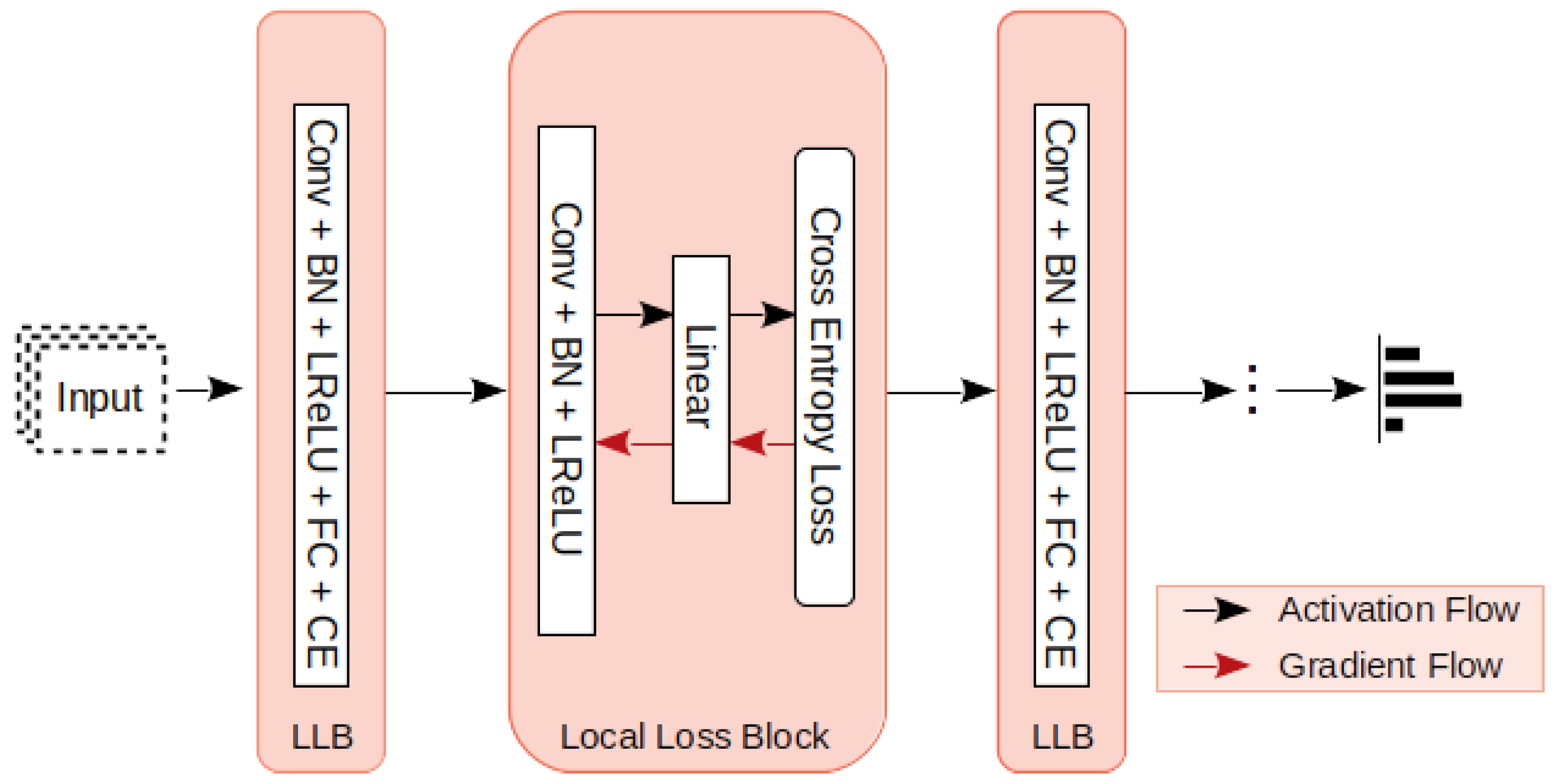
3.1. Local Loss Computation

To compute the local loss, we measure the cross-entropy (CE) between the local classifier predictions and the target. Our PrimeNet design has four intermediate classifiers that separately predict the output and compute the loss for the same one-hot-encoded target. We represent local loss as $L_{local}$, and this can be defined as given below:

$$L_{local}=CE(y_i,f(x_i;\theta )),$$

(1)

where $Y_i$ is the one-hot-encoded target, and $f(x_i;\theta )$ is a result of the previous activation. We flattened the feature maps and applied soft-max activation to obtain the local loss in PrimeNet. To perform backpropagation free, layer-wise training, we detached the computation graph to stop the gradient flow. Weights are updated using the cross-entropy loss function. Adam [29] optimizer is used with $\beta$ set to 0.99.

3.2. Convolution with Local Loss

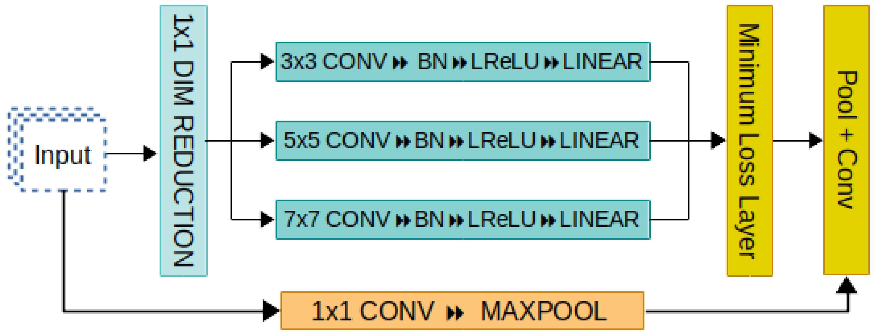
Our proposed PrimeNet is a multiscale, backwards-locking free, adaptive inference neural structure. PrimeNet can be used with other traditional convolution layers, but the standard convolution and hidden layer weights are updated by sending the gradients back to the previous layers through the backpropagation process, and PrimeNet updates the weights layer-wise. To facilitate the end-to-end backpropagation free convolution operation in PrimeNet, we customized and used a standard convolution layer enabled with inline layer-wise training [4].

Each layer respective to each feature scale in PrimeNet block is constituted of this custom convolution operation enabled with local loss update within local loss block (LLB). The $CONV\to BN\to LReLU\to FC\to SOFTMAX$ layer sequence is followed in order to compute the local loss. Here, CONV refers to the convolution layer, and BN refers to the batch normalization operations. LReLU is the activation function, and FC (fully connected) refers to the dense layer operation just before the softmax classifier.

3.3. PrimeNet

In the proposed PrimeNet framework, the shallow, deep learning structures work as a catalyst in the overall learning of the primary discriminative network. The capsule-like shallow structures present multiscale feature representations, and the dynamic selection logic encourages the representations with immediate minimum local loss. The learned feature representation is dynamically added to the secondary classifier network, which benefits the model into faster convergence. To design the PrimeNet block, we first set up the conditional computation model with multiple intermediate classifiers. Each classifier in this arrangement operates on a different feature scale. The shallow Local Loss Block layer order ($CONV\to BN\to LReLU\to FC\to SOFTMAX$) from Figure 1 is followed to compute local loss from each intermediate classifier.

From Figure 2, it can be seen that larger filter sizes (namely 5 × 5 and 7 × 7) are used, which will result in an increased number of parameters and require more computation power. A 1 × 1 convolution layer is used just after the input for dimensionality reduction, while retaining the salient features from the input. The memory and computational savings by dimensionality reduction allowed us to use a $3\times 3$ projection further to pool features across the channels and increase feature maps.

Translation invariant feature projection: The convolution layer feature maps, unlike dense layers, are inherently insensitive to the location of the features in the input [2,30,31]. There may be chances that the loss-based conditional computation may always choose and concentrate in a particular local region. Moreover, the proposed multiscale feature abstraction process distills the most prominent visual indicators set, and the remaining features of the other layers are soft pruned. Sometimes, soft pruning could also result in the loss of essential features, which is a problem known as extreme compression.

The translation invariance in CNN is achieved by combining the convolution and maxpooling layer operations. The convolution layer convolves through an image patch and abstracts the features with their respective position. After that, max-pooling filters out the max value of the feature from the convolved output and reduces the dimension and complexity. By obtaining the max-value, it inherently discards the positional information of the features, which makes it translation invariant.

In the proposed research, we innovatively used the translation invariance of the input, projected with input features of the same image. This helped our adaptive convolution design to avoid the correlated units being concentrated in the same region. The projection layer also reduces the effect of extreme compression caused by soft pruning and presents a normalized local translation invariant feature presentation of the same input.

To implement the adaptive convolution strategy, we set up our conditional computation block as a primary external network which consists of four intermediate classifiers respective to each feature scale. Each intermediate classifier (named a capsule network) implements the shared input for the same target output. The proposed PrimeNet architecture multiscale micro-network operates to perform intermediate classifications. Local loss is computed for each scale convolution, and the adaptive convolution is performed. The other layers with higher losses are soft pruned, and their weights are locally updated.

$$[y_1,y_2,y_3,y_4]=f(x;\theta )=[f_1(x;{\theta }_1),...,f_4(x;{\theta }_4)],$$

(2)

where x is the input image, and f${(}_1{,}_2{,}_3{,}_4)$ and $\theta {(}_1{,}_2{,}_3{,}_4)$ represents the transformation operation (conv → fc → softmax) for y${}_i$ classifier. Now, each capsule operates on same input images for the same classifier output, and Equation (2) can be reduced as following:

$$\left[y\right]=f_i(x;\theta )];$$

(3)

here, $f_i$ represents the transformation operation at i-th convolution scale for the same y target output. Similarly, from Equation (1), the loss function can be expanded here as

$$L(y,f(x;\theta ))=CE[y_1\left(f_1(x;{\theta }_1)\right),...,\left(y_4\left(f_4(x;{\theta }_4)\right)\right];$$

(4)

which is further reduced as:

$$L_i(y,f_i(x;\theta ))=CE\left[y\left(f_i(x;{\theta }_1)\right)\right]$$

(5)

here, $L_i(y,f_i(x;\theta ))$ represents the loss as a result of a cross-entropy operation between the i-th scale convolution output prediction and the expected prediction. After this, the loss based adaptive inference is implemented as a simple if-then-else operation, and the following selected convolution layer is written as:

$$f_{min}(x;\theta )=MIN\left[L(y,f(x;\theta ))\right].$$

(6)

Once the local predictions are made, and the min-loss layer is identified, the next challenge is to extract the min-loss features. To address this issue, we provisioned our capsule network instances to generate predictions along with their raw convolution feature output. After the min-loss layer is identified, the generated convolution feature output is taken and forwarded to be used by the next layer. At this stage, we obtain the most prominent visual indicators. Typically, an iterative algorithm overfits when the network is too complex or algorithm runs for too long [32]. By complex network, we refer that it is over parameterized. The capsule network’s decoupled local weight training and update have an advantage here: it prevents the classifier model’s overlearning. The disconnected training ensures that the model is simple and not too complex. In addition, the capsule instances do not participate in classifier model weight training which prevents over parameterization of the network. This means the capsule instances are trained per batch per iteration, and their previous weights are discarded once the min-loss features are extracted for every epoch. By disconnected training design, the simplicity of the network with reduced parameters is achieved. Now, the translation invariant feature projection can be applied as follows:

$$f_{next}(x;\theta )=\left[f_{min}{(x;\theta )}^{⌢}S(x;\theta )\right],$$

(7)

where $f_{next}(x;\theta )$ is the next layer input after concatenation (${}^{⌢}$) of convolution output with minimum loss $f_{min}(x;\theta )$ and pool projection $S(x;\theta )$.

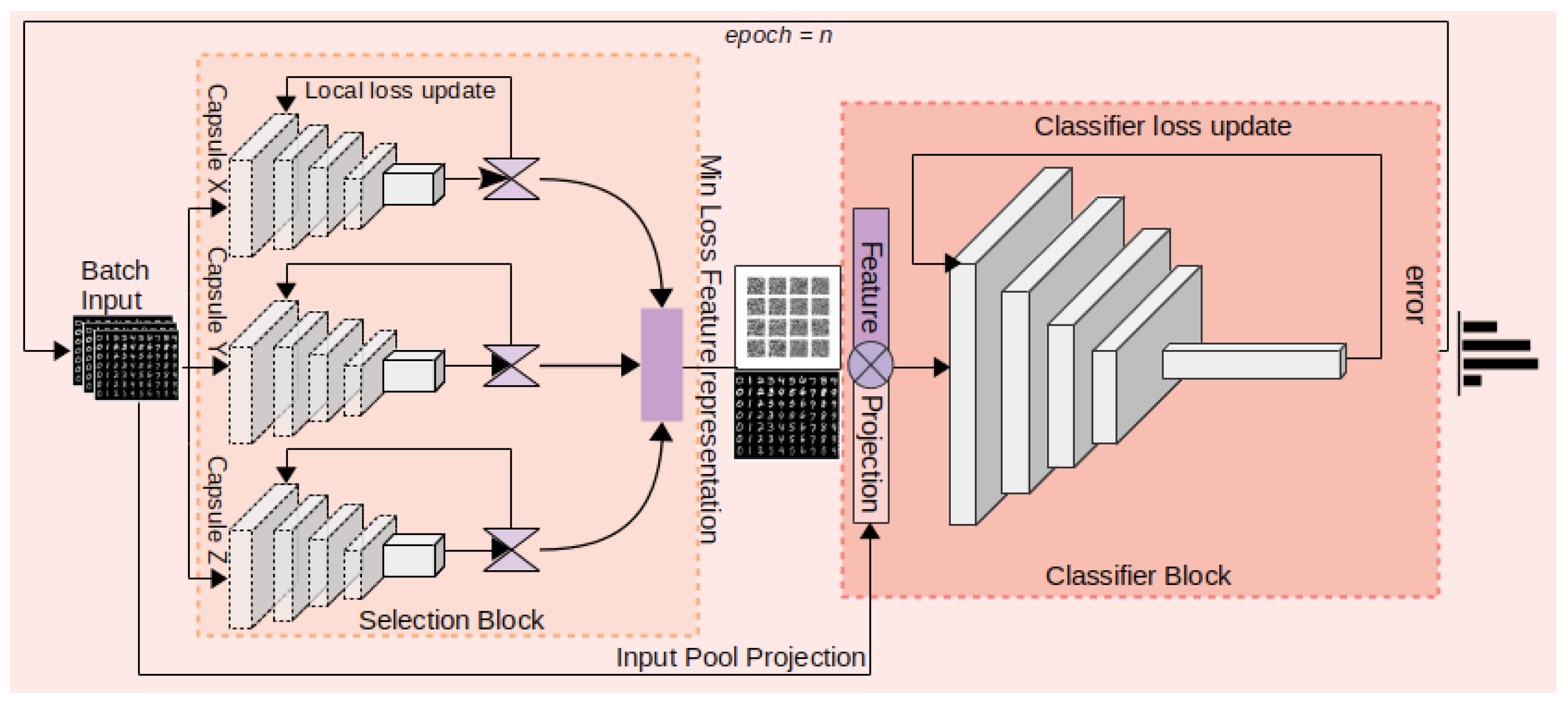
3.4. Feature Representation with Minimum Loss Local Structure Transferring

To implement the PrimeNet framework, we divided the training design into two parts (Figure 3). In the first part, we implemented a multiscale shallow neural structure for reusable feature representation. Each shallow neural, structure termed as capsule, will learn a feature representation at a specific convolutional scale. The simultaneous feature representations will be analyzed for minimum batch input loss. The minimum loss feature representation will be forwarded to be inculcated in the second part of the model design. The weights for each lightweight network will be updated there itself using the local loss update procedure. The secondary part of the design is an instance of the PrimeNet classifier that takes the selected minimum loss feature representation as input and concatenates it with the batch input projection. With this feature projection, a summarized local translation invariant feature representation is obtained. The features are flattened, and a linear representation with a softmax activation function is used to obtain classification output.

3.5. Learning Algorithm

Various substantial implementation settings have been studied to design the learning algorithm, including non-linear model topologies, shared input, and multiple model inputs and outputs. Typically, a deep learning model is a compound directed acyclic graph (DAG) structure of different layers. An extension to DAG is to build graphs of layers. In our training routine (Algorithm 1), the proposed deep learning structure runs multiple instances non-linearly and shares the input. We reused the unit architecture and its weights by running the multiple instances of the proposed PrimeNet structure.

Algorithm 1 Training algorithm for classifier model.
Input: Batch Images
Output: Prediction
1: procedure TRAIN( )
2:     capsuleX=Capsule()	▷ Shallow network instance for x scale.
3:     capsuleY=Capsule()	▷ Shallow network instance for y scale.
4:     capsuleZ=Capsule()	▷ Shallow network instance for z scale.
5:     classi f ier=PrimeNet()	▷ Classifier Network Instance.
6:     procedure FEATURE_TRAIN(images)	▷ Individual capsule training for feature generarion
7:         featuresX = capsule(images)	▷ Features X from Capsule X.
8:         lossX = loss( featuresX)	▷ loss from feature X.
9:         featuresY = capsule(images)	▷ Features Y from Capsule Y.
10:       lossY = loss( featuresY)	▷ loss from feature Y.
11:       featuresZ = capsule(images)	▷ Features Z from Capsule Z.
12:       lossZ = loss( featuresZ)	▷ loss from feature Z.
13:       if (lossX < lossY)&(lossX < lossZ) then
14:       min_loss_ features=featureX
15:       else if (lossY > lossX)&(lossY > lossZ) then
16:           min_loss_ features=featureY
17:       else
18:           min_loss_ features=featureZ
19:       end if
20:       gradient_update(capsuleX, capsuleY, capsuleZ)	▷ local gradient update
21:     end procedure
22:     for epoch in range(epochs) do
23:       classifier_loss = 0
24:       total_classifier_loss = 0
25:       for batch_images in train_dataset do
26:           MinLossFeature=feature_train(batch_images)
27:           features=MinLossFeature + input_projection	▷ Input feature projection is concatenated.
28:           classifier_output = classifier( features)
29:           classifier_loss = loss(classifier_output)
30:           total_classifier_loss += classifier_loss	▷ Combined classifier loss
31:           update_weights=gradient_update(classifier)
32:       end for
33:     end for
34: end procedure

Further, to learn from the local multiscale representations (Capsule instances) and transfer the encoding for final classification (classifier model), our iterative training strategy chains the dynamically selected capsule output with the classification model. In the first part, we trained the batch input through the proposed selection network block (Figure 3) and obtained the local representation for local loss computation. After computation of the local loss, we compared the capsule for minimum loss and transferred the capsule instance’s convoluted output to the classifier block. In the classifier part of the training, the selected convolved output from the capsule is concatenated with input feature projection. The input feature projection presents a local translation-invariant version of the input, which further balances the domination of correlated regions in overall feature representation. The rest of the classifier block is designed as a simple convolutional network that facilitates a swift classification of dynamically learned feature representations.

4. Experiments and Results

Our experiments present the PrimeNet as a shallow multiscale neural structure mainly to obtain the input’s prime discriminative characteristics. We also present the backpropagation free layer-wise gradient update procedure within PrimeNet, which combines with the other traditional layers and allows the weight update alternatively with the traditional backpropagation method. To evaluate the performance of the representation learning algorithm, we used PrimeNet as a feature extractor on various benchmarked datasets and evaluated the performance of linear models fitted on top of these features. Moreover, we visualize and compare the feature representations generated by PrimeNet and ResNet models using t-Distributed Stochastic Neighbor Embedding (t-SNE) [33] feature visualizations. Finally, we presented the result analysis by comparing with different considered baseline performances.

4.1. Implementation Details

We utilized three simultaneous multiscale capsule-like networks in the initial step by following the structure from Figure 1 ($Conv\to BN\to LReLU\to Flatten\to Dense$). For every iteration, one input batch is fed as an input to these shallow capsules. These small networks are trained with batch input, and we extract the feature representation occurring minimum loss from the convolved output of the same capsule. The selected feature representation is concatenated with input feature projection. The projection function $S(x;\theta )$ in Equation (7) is implemented as the maxpool2D → conv2D with ReLU activation function. The capsule and PrimeNet’s classifier model information is provided in the table below:

Here, the parameter column refers to the convolution scales and number of filters (e.g., 1 × 1 is the convolution scale, and 32 is the number of filters). NA means that there are no trainable parameters involved. GAP refers to the meaning Global Average Pooling in the Classifier configuration.

We set the maximum iteration for 100 epochs in the training phase and use a mini-batch of size 200. For fine-tuning and evaluation, we use 50 iterations and a reduced batch size of 32. Moreover, we use the Adam optimizer with a default learning rate of 0.0002 with a beta value of 0.99. To recreate and compare with baseline ResNet50 and other SOTA models for computational results, we reshaped the MNIST input into three dimensions as per the experimental requirement. No data augmentation is used in PrimeNet experiments for any of the three datasets.

4.2. Experimental Setup

We selected three datasets for our experiments, which includes MNIST, CIFAR-10, and SVHN. The model information of shallow network (Capsule; works as an enhanced feature extractor) and main classifier network is presented in

Table 1. Capsule and classifier model configuration information.

Capsule (Shallow Network)		PrimeNet (Classifer)
Layer	Parameter	Layer	Parameter
Conv2D	1 × 1, 32	MaxPool	3 × 3
Conv2D	3 × 3, 5 × 5, 7 × 7, 64	Conv2D	1 × 1, 64
BN	NA	BN	NA
LReLU	NA	MaxPool	2 × 2
Flatten	NA	Conv2D	3 × 3, 128
Dense	28 × 28 × 1, 32 × 32 × 3	GAP	NA
		Flatten	NA
		Dense	10

. A brief description of the datasets is in the following table (

Table 2. Summary of the datasets used for the experiments.

Dataset	Input Size	No. of Classes	Train Size	Test Size
MNIST	28 × 28 × 1	10	60,000	10,000
CIFAR-10	32 × 32 × 3	10	50,000	10,000
SVHN	32 × 32 × 3	10	73,257	26,032

).

4.3. Results

Table 3. Comparison of classification error rate on evaluation model (%). The symbols $\left(\mu \right)$ and $\left(\sigma \right)$ represent the mean and standard deviation, respectively, for the top 5 scores from each dataset.

Dataset	PrimeNet Test Error (%)			Model	Baseline Error (%)	Baseline Method
	Top-1	Top-5 ($\mathit{\mu }$)	$\mathit{\sigma }$
MNIST	0.59	0.706	0.14	DT-RAM [12]	1.46, 1.12	Conditional Computation
				Condensenet [18]	3.46, 3.76	Conditional Computation
				ITADN [17]	5.9	Conditional Computation
CIFAR-10	6.21	7.34	3.67	RNP [7]	15.05	Network Pruning
				SFP [21]	7.74, 6.32	Network Pruning
				ITADN [17]	3.13, 5.99	Knowledge Distillation
SVHN	1.71	2.2	0.42	ONE [27]	1.63	Knowledge Distillation

presents the obtained error rate performances of different state-of-the-art network models in the category of three related techniques, comparing with the proposed PrimeNet learning algorithm. We run the PrimeNet algorithm for several repetitions and recorded the top-1 and top-5 results with their mean (μ) and standard deviation (σ). For the MNIST digits dataset, PrimeNet has obtained a record top-1 performance surpassing all the results from considered baselines. MNIST is assumed to be too easy, but it is our first choice to test our algorithm because, if an algorithm fails on MNIST, it is likely to fail on other tests. To further evaluate the performance of the proposed algorithm, we tested it on the Street View House Number (SVHN) dataset. With SVHN, the PrimeNet has obtained an acceptable performance close to the considered state-of-the-art method. We also evaluated our algorithm on the CIFAR-10 dataset for more generalized observations. This is to note that the state-of-the-art results are obtained without using any data preconditioning, and the input batches are shuffled while loading datasets.

The observations are: (1) The proposed PrimeNet structure acts as a helper network for obtaining the prime visual indicators from the input and is most suitable for early convolution stages. PrimeNet is helpful to reduce the size of large deep networks with lesser weight adjustment operations. (2) The PrimeNet is an independent adaptive deep neural structure with its own backpropagation free gradient update technique. PrimeNet infers that the complex deep neural networks can comprise a backwards-locking free mechanism to reduce computational complexities further. (3) The experiments also suggest that the standard convolutional layers can be easily replaced or combined with PrimeNet.

4.4. Computational Analysis

While achieving the state-of-the-art results, we have significant gains on the computational efficiency of the proposed algorithm. To evaluate the computational efficiency, we have considered and compared three key characteristics from each model. The considered characteristics are (i) number of FLOPs (floating-point operations), (ii) model parameters, and (iii) memory requirement.

Table 4. Summary of the computational results for MNIST, CIFAR-10, and SVHN experiments.

Model	Dataset	Params (Millions)	FLOPs (Millions)	Epochs
ResNet [34]	All Three	23.6	409	50
PrimeNet (Ours)	All Three	0.41	2.7	100 + 50
Condensenetlight [18]	CIFAR-10	0.33	122	300
Condensenet86 [18]	CIFAR-10	0.52	65	300
ONE [27]	SVHN	0.5	2.28	300, 40

(Tensorflow or Keras model’s computational information is obtained using model profiler function available at https://pypi.org/project/model-profiler/, accessed on 7 October 2021) presents the computational gains achieved by PrimeNet and compares them with different considered baseline results, depending on the information available in the original paper. The majority of related research results are obtained using ResNet architecture as a base model, so we also considered ResNet50 computational results as the first baseline to be compared. RestNet50 with pre-trained Imagenet weights has been recreated for our task data classifier with the same settings for each experiment.

Here, we have considered the combined computational information from the shallow dynamic deep neural structure and its classifier for computational analysis. Hence, the number of epochs for our algorithm is 100 + 50, which means 100 iterations for classifier network using shallow PrimeNet structure. Once the learned feature representation is extracted from the classifier, another 50 epochs are used for retraining. ResNet is trained for 50 epochs for the same purpose, and other baselines take 300 minimum epochs. Since we have used the same architecture for PrimeNet and ResNet baseline, we obtained the same number of parameters and FLOPs for all datasets. ResNet is one sizeable deep network that involves the highest computational cost. ONE [27] has produced the computational information for the experiment on SVHN, which has a precise, reduced number of FLOPs, whereas PrimeNet is just 15% costlier, but, on the other side, PrimeNet can reduce to number of parameters by 18%. Similarly, for Cifar-10, $Condensene{t}^{light}$ [18] can reduce the parameter size by 20% from PrimeNet, but PrimeNet has a tremendous gain of almost 99% reduced number of FLOPs. For another Condensenet experiment on the same dataset, PrimeNet has obtained almost 20% parameters and 95% FLOPs gain. Thus, the experiments suggest the proposed method’s efficacy in various computational and classification performance categories (Table 4).

5. Ablation Study

We perform an ablation study on MNIST data in which we investigate (1) the simultaneous local gradient updates from each PrimeNet instance with the effect of dynamic selection on the classifier network and (2) the quality of resultant features extracted from the classifier network to be used for evaluation and compared it with the ResNet50 feature visualization.

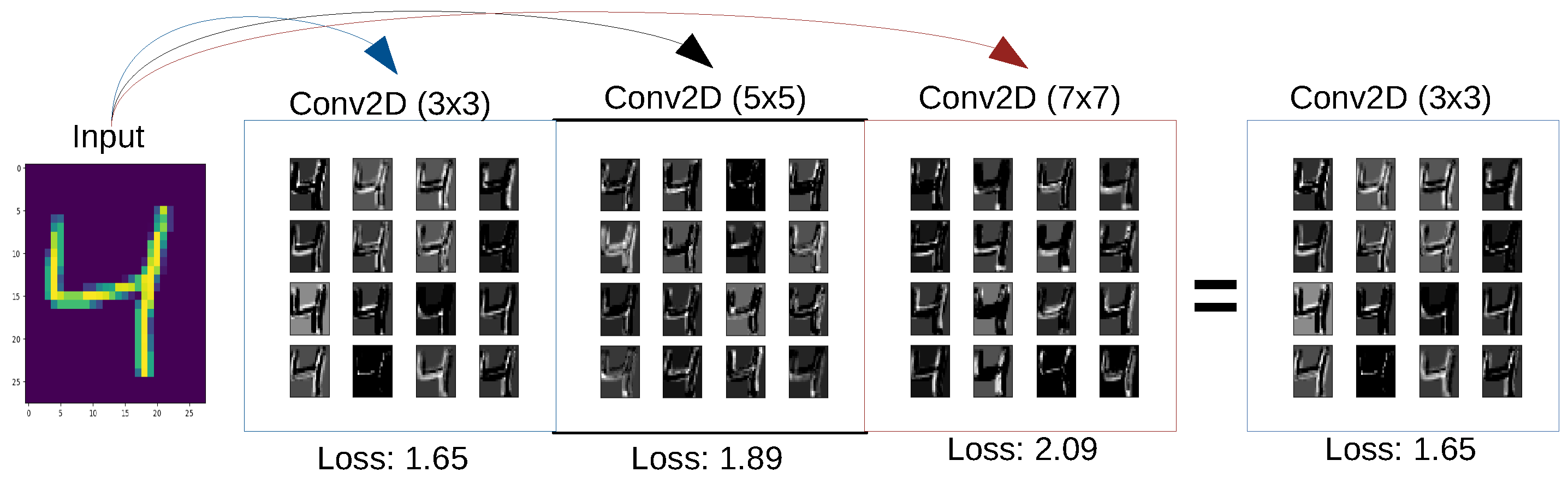
5.1. Local Gradient Update

The local gradient update strategy is simple and straightforward. The capsule-like instances are capable of computing the layer-wise loss. Since these tiny networks are decoupled from the training loop, the local layer loss is computed as described in Equation (5). Figure 4 presents qualitative results for a single input instance. To generate the feature maps as qualitative output, we accessed the layer attributes within the PrimeNet structure of the model. To identify the exact layer within the PrimeNet structure, the model summary comes as a handy tool. The features maps are nothing, but the weights and deep learning models have layer weight attributes with which the weights are accessible. We have visualized sixteen feature maps (16 filter activations) from each PrimeNet layer (particularly the convolution layer) and normalized their values to visualize them easily. For the same input instance, the proposed PrimeNet design is able to compute the losses. With the help of visualization libraries, the feature maps are plotted.

In the training phase, we visualized the gradient updates by recording the loss values of each capsule in each iteration, along with the resulting classifier’s total loss value. The total loss of the classifier is the dynamically selected capsule loss added with the classifier’s loss (Figure 5). This result shows the gradual loss update from all the intermediate capsule-like networks and their cumulative effect on the classifier model.

5.2. Adaptive Cost-Conscious Local Structure Transfer

To exhibit the efficiency of the cost-conscious local structure transfer technique, we extracted learned feature representations by the proposed PrimeNet. We extracted the trained representation of the features and performed clustering using t-SNE visualization and then compared it with the ResNet50 baseline. From Figure 6, this can be observed that the extracted feature representation using PrimeNet has more clear cluster margins than the ResNet features, proving that it could lead models to converge faster and obtain promising classification test results.

To further support the experimental evidence, we also visualized the learned feature representation of a single random train image. The learned feature output is extracted simply by obtaining the convolution output just before the linear operation (FC + Softmax). The sample input image is evaluated, and the headless model generates the feature maps. The extracted feature map is reshaped into the original shape (e.g., MNIST 28 × 28 × 1) as presented in Figure 7. We also presented the learned feature visualization of the same image using the ResNet model using the same method (Figure 8).

Figure 9 presents the impact of our adaptive convolution selection strategy over the linear convolution neural networks. The classifiers with standard convolution layers are presented with labels Layer 3 × 3, Layer 5 × 5, Layer 7 × 7, and the evaluation model’s loss is presented with label train_acc and train_loss.

Figure 9 also reflects the learned feature representation extracted from the secondary classifier has resulted in faster convergence and fewer epochs (less than 10).

6. Conclusions

In this research, we introduced a flexible deep neural structure called PrimeNet. PrimeNet is an efficient convolutional neural network design that encourages strong visual indicators and reusing the same via backpropagation free convolutional layers. With its learned multiple multiscale convolutions, it attempts to soft prune the filters with less valuable features. The simplistic adaptive and cost-conscious local structure transfer technique can reduce the overall computational cost of the models while retaining the latest SOTA performance. Due to its simple implementation, the PrimeNet structure replaces traditional convolutional layers, combining the local or global gradient update methods. There are specific suggested future directions in which we would like to extend this research. (1) The PrimeNet can headway complex modules as layers, such as Inception, Attention, or Residual modules. (2) PrimeNet can lead to finding several other conditional computing operations in different applications.

References

1. Lin, M.; Chen, Q.; Yan, S. Network in network. arXiv 2013, arXiv:1312.4400. [Google Scholar]
2. Szegedy, C.; Liu, W.; Jia, Y.; Sermanet, P.; Reed, S.; Anguelov, D.; Erhan, D.; Vanhoucke, V.; Rabinovich, A. Going deeper with convolutions. In Proceedings of the IEEE Conference on Computer Vision and Pattern Recognition, Boston, MA, USA, 7–12 June 2015; pp. 1–9. [Google Scholar]
3. Rosenblatt, F. Principles of Neurodynamics. Perceptrons and the Theory of Brain Mechanisms; Technical Report; Cornell Aeronautical Lab. Inc.: Buffalo, NY, USA, 1961. [Google Scholar]
4. Nøkland, A.; Eidnes, L.H. Training neural networks with local error signals. In Proceedings of the International Conference on Machine Learning, PMLR, Long Beach, CA, USA, 9–15 June 2019; pp. 4839–4850. [Google Scholar]
5. Bolukbasi, T.; Wang, J.; Dekel, O.; Saligrama, V. Adaptive neural networks for fast test-time prediction. arXiv 2017, arXiv:1702.07811. [Google Scholar]
6. Huang, G.; Chen, D.; Li, T.; Wu, F.; van der Maaten, L.; Weinberger, K.Q. Multi-scale dense networks for resource efficient image classification. arXiv 2017, arXiv:1703.09844. [Google Scholar]
7. Lin, J.; Rao, Y.; Lu, J.; Zhou, J. Runtime neural pruning. In Proceedings of the 31st International Conference on Neural Information Processing Systems, Long Beach, CA, USA, 4–9 December 2017; pp. 2178–2188. [Google Scholar]
8. Wang, X.; Yu, F.; Dou, Z.Y.; Darrell, T.; Gonzalez, J.E. Skipnet: Learning dynamic routing in convolutional networks. In Proceedings of the European Conference on Computer Vision (ECCV), Munich, Germany, 8–14 September 2018; pp. 409–424. [Google Scholar]
9. Veit, A.; Belongie, S. Convolutional networks with adaptive inference graphs. In Proceedings of the European Conference on Computer Vision (ECCV), Munich, Germany, 8–14 September 2018; pp. 3–18. [Google Scholar]
10. Figurnov, M.; Collins, M.D.; Zhu, Y.; Zhang, L.; Huang, J.; Vetrov, D.; Salakhutdinov, R. Spatially adaptive computation time for residual networks. In Proceedings of the IEEE Conference on Computer Vision and Pattern Recognition, Honolulu, HI, USA, 21–26 July 2017; pp. 1039–1048. [Google Scholar]
11. Kong, S.; Fowlkes, C. Pixel-wise attentional gating for parsimonious pixel labeling. arXiv 2018, arXiv:1805.01556. [Google Scholar]
12. Li, Z.; Yang, Y.; Liu, X.; Zhou, F.; Wen, S.; Xu, W. Dynamic computational time for visual attention. In Proceedings of the IEEE International Conference on Computer Vision Workshops, Venice, Italy, 22–29 October 2017; pp. 1199–1209. [Google Scholar]
13. Ying, C.; Fragkiadaki, K. Depth-adaptive computational policies for efficient visual tracking. In International Workshop on Energy Minimization Methods in Computer Vision and Pattern Recognition; Springer: Berlin/Heidelberg, Germany, 2017; pp. 109–122. [Google Scholar]
14. Wu, Z.; Nagarajan, T.; Kumar, A.; Rennie, S.; Davis, L.S.; Grauman, K.; Feris, R. Blockdrop: Dynamic inference paths in residual networks. In Proceedings of the IEEE Conference on Computer Vision and Pattern Recognition, Salt Lake City, UT, USA, 18–22 June 2018; pp. 8817–8826. [Google Scholar]
15. McIntosh, L.; Maheswaranathan, N.; Sussillo, D.; Shlens, J. Recurrent segmentation for variable computational budgets. In Proceedings of the IEEE Conference on Computer Vision and Pattern Recognition Workshops, Salt Lake City, UT, USA, 18–22 June 2018; pp. 1648–1657. [Google Scholar]
16. Kang, D.; Dhar, D.; Chan, A.B. Incorporating Side Information by Adaptive Convolution. Int. J. Comput. Vis. 2020, 128, 2897–2918. [Google Scholar] [CrossRef]
17. Li, H.; Zhang, H.; Qi, X.; Yang, R.; Huang, G. Improved techniques for training adaptive deep networks. In Proceedings of the IEEE/CVF International Conference on Computer Vision, Seoul, Korea, 27–28 October 2019; pp. 1891–1900. [Google Scholar]
18. Huang, G.; Liu, S.; Van der Maaten, L.; Weinberger, K.Q. Condensenet: An efficient densenet using learned group convolutions. In Proceedings of the IEEE Conference on Computer Vision and Pattern Recognition, Salt Lake City, UT, USA, 18–22 June 2018; pp. 2752–2761. [Google Scholar]
19. Mnih, V.; Heess, N.; Graves, A.; Kavukcuoglu, K. Recurrent models of visual attention. arXiv 2014, arXiv:1406.6247. [Google Scholar]
20. Khan, F.U.; Aziz, I.B.; Akhir, E.A.P. Pluggable Micronetwork for Layer Configuration Relay in a Dynamic Deep Neural Surface. IEEE Access 2021, 9, 124831–124846. [Google Scholar] [CrossRef]
21. He, Y.; Kang, G.; Dong, X.; Fu, Y.; Yang, Y. Soft filter pruning for accelerating deep convolutional neural networks. arXiv 2018, arXiv:1808.06866. [Google Scholar]
22. Singh, P.; Verma, V.K.; Rai, P.; Namboodiri, V.P. Play and prune: Adaptive filter pruning for deep model compression. arXiv 2019, arXiv:1905.04446. [Google Scholar]
23. Lin, M.; Ji, R.; Zhang, Y.; Zhang, B.; Wu, Y.; Tian, Y. Channel pruning via automatic structure search. arXiv 2020, arXiv:2001.08565. [Google Scholar]
24. Wang, L.; Dong, X.; Wang, Y.; Ying, X.; Lin, Z.; An, W.; Guo, Y. Exploring Sparsity in Image Super-Resolution for Efficient Inference. arXiv 2021, arXiv:2006.09603. [Google Scholar]
25. Kim, J.; Chang, S.; Yun, S.; Kwak, N. Prototype-based Personalized Pruning. arXiv 2021, arXiv:2103.15564. [Google Scholar]
26. Luo, C.; Zhan, J.; Hao, T.; Wang, L.; Gao, W. Shift-and-Balance Attention. arXiv 2021, arXiv:2103.13080. [Google Scholar]
27. Lan, X.; Zhu, X.; Gong, S. Knowledge distillation by on-the-fly native ensemble. arXiv 2018, arXiv:1806.04606. [Google Scholar]
28. Hinton, G.; Vinyals, O.; Dean, J. Distilling the knowledge in a neural network. arXiv 2015, arXiv:1503.02531. [Google Scholar]
29. Kingma, D.P.; Ba, J. Adam: A Method for Stochastic Optimization. arXiv 2017, arXiv:1412.6980. [Google Scholar]
30. Springenberg, J.T.; Dosovitskiy, A.; Brox, T.; Riedmiller, M. Striving for Simplicity: The All Convolutional Net. arXiv 2015, arXiv:1412.6806. [Google Scholar]
31. Yosinski, J.; Clune, J.; Bengio, Y.; Lipson, H. How transferable are features in deep neural networks? arXiv 2014, arXiv:1411.1792. [Google Scholar]
32. Panchal, G.; Ganatra, A.; Shah, P.; Panchal, D. Determination of over-learning and over-fitting problem in back propagation neural network. Int. J. Soft Comput. 2011, 2, 40–51. [Google Scholar] [CrossRef]
33. Van der Maaten, L.; Hinton, G. Visualizing Data using t-SNE. J. Mach. Learn. Res. 2008, 9, 2579–2605. [Google Scholar]
34. He, K.; Zhang, X.; Ren, S.; Sun, J. Deep Residual Learning for Image Recognition. arXiv 2015, arXiv:1512.03385. [Google Scholar]
Figure 1. The backward-locking free, custom convolution block that updates the layer-wise local loss instead of sending the gradients back through backpropagation. Redrawn from figure source in Reference [4].
Applsci 12 01842 g001
Figure 2. The proposed PrimeNet architecture. Multi-scale micro-network operates to perform intermediate classifications. Local loss is computed for each scale convolution, and the adaptive convolution is performed. The other layers with higher losses are soft pruned, and their weights are locally updated.
Applsci 12 01842 g002
Figure 3. PrimeNet training flow. The shallow capsules network inside the selection block convolves at different scales, and the batch-wise loss is calculated as gradients are updated locally. The feature representation with minimum loss is forwarded as an input to the classifier, and classification is performed on locally learned feature representation.
Applsci 12 01842 g003
Figure 4. Qualitative output and dynamic selection strategy for capsule-like shallow networks.
Applsci 12 01842 g004
Figure 5. Visualization of local gradient updates from shallow and classifier networks.
Applsci 12 01842 g005
Figure 6. The t-SNE visualization of features from image representations by proposed PrimeNet (a) and ResNet50 (b).
Applsci 12 01842 g006
Figure 7. Visualization of learned feature representation using PrimeNet’s classifier model.
Applsci 12 01842 g007
Figure 8. Visualization of learned feature representation using ResNet model.
Applsci 12 01842 g008
Figure 9. (a,b) The incremental model learning from the dynamically selected feature representations as a result of fine tuning on top of the classifier. Linear classifier network (static convolutional) losses and accuracies are also presented to demonstrate the difference in performance.
Applsci 12 01842 g009