Article

Advanced Thermal Manikin for Thermal Comfort Assessment in Vehicles and Buildings

1
INCAS—National Institute for Aerospace Research “Elie Carafoli”, B-dul Iuliu Maniu 220, 061136 Bucharest, Romania
2
CAMBI Research Center, Building Services Department, Technical University of Civil Engineering Bucharest, 66 Avenue Pache Protopopescu, 021414 Bucharest, Romania
3
Department of Mechanical Engineering, Technical University of Cluj Napoca, 101–103 Muncii Avenue, 400020 Cluj-Napoca, Romania
*
Authors to whom correspondence should be addressed.
Appl. Sci. 2022, 12(4), 1826; https://doi.org/10.3390/app12041826
Submission received: 21 November 2021 / Revised: 28 December 2021 / Accepted: 28 December 2021 / Published: 10 February 2022
(This article belongs to the Special Issue Urban Sustainability and Resilience of the Built Environments)

Abstract

:

Featured Application

Thermal comfort assessment in vehicles and buildings and other transient thermal environ-ments.

Abstract

Among the factors that influence the resilience and sustainability of cities in general, and of inhabited spaces in particular, there are extreme temperatures and, in particular, for people, thermal comfort is something that should be considered. This problem includes all aspects of comfort for users of inhabited spaces in both buildings and vehicles. The purpose of this paper is to present the details of a recently designed and created thermal manikin that comprises 79 superficial zones with independent neuro-fuzzy temperature regulation. Both the component parts of the manikin and the acceptance strategy are described. Flexible heating elements were used to control the temperature, on which five digital sensors are positioned. In order to establish the relationship between heat loss and ambient temperature, the thermal manikin was calibrated in a climatic chamber. The thermal manikin was able to predict local sensations through the equivalent temperature concept of the so-called Predicted Mean Vote.

1. Introduction

1.1. General Considerations about the Thermal Comfort and Its Assessment

Thermal comfort is a complicated concept and can be described by a multitude of sensations that are provided by a multitude of factors that influence the thermal state that is experienced by humans. It is therefore quite difficult to find a universal definition for this concept, and there are several definitions for thermal comfort in the literature. Sometimes, thermal comfort is explained as “ambient conditions for which a person would not prefer a different environment [1]”. The definition that is offered by the American ASHRAE 55 standard [2] presents thermal comfort as “a subjective concept of well-being generated by the balance between the body and the environment”. Thermal comfort demonstrates statistical content in the sense that it characterizes the fact that a significant percentage of a group of people consider an environment as being comfortable when defined by those parameters [3]. In this way, one could define thermal comfort as the relationship between all of the factors that influence the heat exchange between the human body and its ambient temperature. Thus, a distinction can be made between the factors that characterize the human body (age, sex, weight, metabolic rate, type of activity, etc.); factors that are related to clothes such as thermal resistance, material structure, and number of layers; or factors that are related to the environment, such as air temperature, speed, humidity, pressure, intensity, and frequency of turbulence [4,5,6,7]. To achieve thermal equilibrium, the body continuously varies the ratio of heat produced to the heat that is ceded. Maintaining this balance is the first condition that intervenes in establishing a state of thermal comfort.
Fifty years ago, Fanger [5] proposed the first comprehensive study that considered different parameters, including physical activity, degree of clothing, and environmental parameters such as air temperature, humidity and speed, and mean radiant temperature. All of these parameters contribute to the calculation of the Predicted Mean Vote (PMV) and the Predicted Percentage of Dissatisfied (PPD) indices that are standardized in ISO 7730 [4]. However, the calculation of PMV or PPD in the case of nonstationary parameters is inappropriate and, in this case, to evaluate the thermal comfort in confined spaces (buildings, vehicles, etc.), the use of the concept of equivalent temperature (teq) is suggested.
The definition of equivalent temperature is given in American ANSI/ASHRAE standard [2] and in EN ISO14505 Part 2 [8], which is a standard that is dedicated to the assessment of the thermal environment in vehicles. The definitions that are provided in [2,8] state that “equivalent temperature” represents the uniform temperature of an imaginary black enclosure in which an occupant would exchange the same amount of heat by radiation and convection as they would in an actual non-uniform environment (see Figure 1) [2]. In this case, the equivalent and the operative temperature use the same definition. They can both be expressed as an average between the values of the air temperature and the radiant mean temperature when they are weighted using the heat transfer coefficients (convection and radiation) that are between the occupant and the environment [9]. The relationship proposed by Madsen [10] for the calculation of the equivalent temperature for air speeds bigger than 0.1 m/s is:
t e q = 0.55 t a + 0.45 t m r + 0.24 0.75 v a 1 + I c l ( 36.5 t a )
where t a is the temperature of the air (°C); v a is the air speed (as measured with the omnidirectional probe) (m/s); I c l is (the clothing thermal insulation (Clo); and t m r is the mean radiant temperature (°C).
The assessment of the above-mentioned equivalent temperature can be obtained using a thermal manikin, which is also the case for other types of sensors: hot films, ellipsoid sensors, etc., see EN ISO 14505/2 [8]. If we know the values of the air speed, of the relative humidity, the level of activity (metabolic rate), and thermal clothing resistance, a diagram with comfort zones showing the range of the operative temperature can be obtained and found to be acceptable. The definitions of teq are based on works [7,9,11,12]. Such comfort zones are presented in Figure 2 and are based on EN ISO 14505/2 [8] and refers to a case of a vehicle’s HVAC-system used in the following context: cooling mode in summer conditions with the passengers wearing light clothing of 0.6 clo(0.09 (m2K)/W). In the same figure, Figure 2, the context refers to the use of a vehicle’s HVAC-system used in heating mode in winter conditions, with the passengers wearing clothing of 1.0 clo (0.155 (m2K)/W).
However, the real teq cannot be directly measured, but there are diverse methods for its approximate determination, but specific definitions are needed that are dependent on the method used. Examples of set-ups are given in Figure 3. In EN ISO 14505/2 [8], the segmental teq for different vehicle conditions is usually determined using two variations of a multi-segmented thermal manikin (Figure 4).

1.2. Thermal Manikins—Standards and Short History

Thermal manikins are used to scientifically test thermal environments, to determine the thermal properties of clothing, f to evaluate the amount of local body heat transfer that occurs in various environments, for example in vehicle cabins, etc. In general, the use of a thermal manikin allows tests to be performed that would be inconvenient for a human subject [13,14,15]. It is important to note and is easy to accept that different manikins will not necessarily produce the same teq value for the same climatic conditions. This can be explained by differences in the construction and in the number of areas and is determined on a case-by-case basis.
Thermal manikins can be used in the automotive industry [7,16,17,18,19], indoor environments [20,21,22,23,24,25], outdoor environments [26,27], and in military [28] and textile research [29]. The history of thermal manikins spans more than 70 years. Their story begins with very simple manikins that were designed to test the clothing intended for American soldiers [28]. Today, the complexity of thermal manikins has increased, and they can closely match the complexity of the human body. The number of independently controlled areas has also increased to 120, see [30]. The materials that are used for the development of thermal manikins have also become more diversified: copper, advanced composite plastic, carbon fiber, and skin-like silicone [31]. Many manikins are designed to simulate the exchange of heat of human body with the environment by measuring heat loss in the immediate environment [28]. Of course, body perspiration and heat exchange by evaporation are, in turn, simulated by high-performance manikins [28,30,32,33]. As performance increases, so does the cost of these tools, allowing for the presence of the human figure to be effectively simulated as well as measurements of the convective and radiative heat transfer coefficients to be taken.
This paper presents the development of an advanced thermal manikin that is based on intelligent neuro-fuzzy control. The development of this prototype started in 2013, in the framework of the EQUATOR project, with subsequent improvements taking place during the QUEST and XTREME projects. This manikin, which is known familiarly as Suzi, is the most advanced of the five different thermal manikin prototypes that have been manufactured in the CAMBI Research Center (Building Services Engineering Faculty, Technical University of Civil Engineering of Bucharest). Studies that have been performed on or with some of these thermal manikins can be found in [34,35,36,37,38]. Suzi was conceived with the help of the INCAS (National Institute of Aerospace Research Elie Carafoli).

2. Design Considerations for the SUZI Prototype

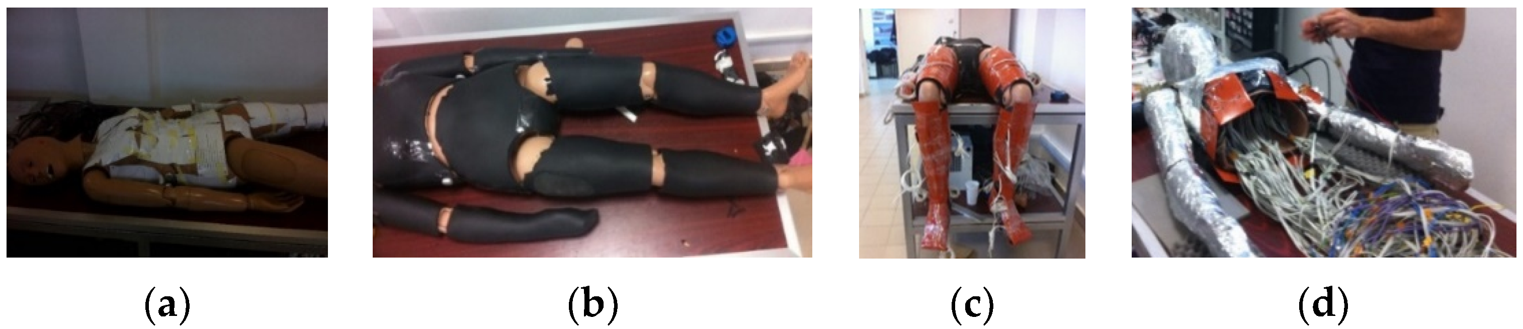
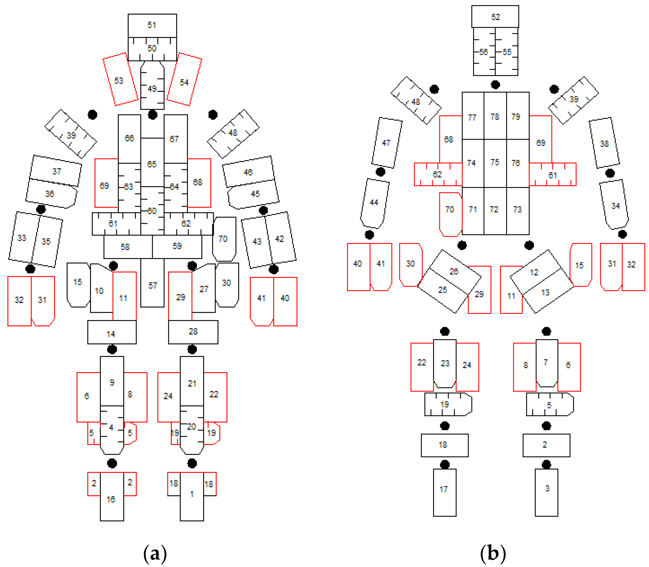
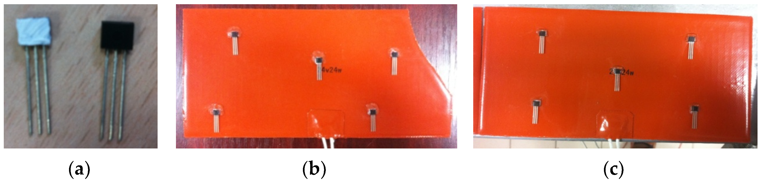
2.1. The Mechanical Structure and the Heating System

This particular manikin prototype was designed and built so that it could be placed in various postures, such as lying down, sitting, or standing positions. The dimensions of this protype were chosen according to the standardized human skin surface of a female human body with a surface area of about 1.8 m2 [20,39]. The main structure is made of polyvinyl, and the surface has been covered with a 5 mm insulation of elastomer membrane (Figure 5b). The role of this membrane is to reduce heat transfer inside the manikin in order to protect the internal electronics from overheating. The hardware components of the thermal prototype were developed in successive stages, as seen in Figure 5a–d).
The upper and bottom body parts were tested, as seen in Figure 6a,b. Four different geometries of elementary flexible patches (Figure 6c) were chosen for the heating system (Figure 6d). The patches were manufactured by the Keenovo Company and consist of a thin layer of silicone (1.5 mm). They include a heating circuit made of nickel chrome heating wire, making them good electrical insulators and good thermal conductors. Of the many solutions that were tested, flexible heating silicone patches proved to be the best choice in ensuring good temperature distribution uniformity. Figure 7 presents the distribution of the HE on the corresponding anatomical areas. The surface of the thermal manikin is divided in 79 areas (or segments) and are intended to be controlled independently. The red drawings represent the zones on the opposite side of the manikin, and the black points illustrate joint points.
The aim was to cover as much of the surface of the manikin as possible without overlapping the patches. The HEs were fixed on the polyvinyl insulation layer using adhesive duct tape. The next step was to create and verify the electrical connection for each body part (hands, legs, etc.). All of the electrical wires were embedded inside the manikin, ensuring their security. The correct operation of each patch was carefully determined through the use of a Lauda Eco Silver thermostatic bath (Figure 8) [40] to characterize the electric circuit resistance variation with temperature. The collected data were necessary to fine-tune the control algorithm (Figure 9).
Five digital temperature sensors were positioned on each heating element to measure the mean temperature as accurately as possible in order to control the patch temperature (Figure 10). TSic T501 model sensors were employed, which were manufactured by the IST company. Given the constructive distribution of the heating elements in the heating patches, there was a risk of biased measurements appearing if the temperature sensors were not installed at suitable positions. Therefore, the position of each sensor position was established using the Flir E40 thermal vision camera to obtain a representative value of the average temperature for the five sensors.
Figure 11 depicts the response of eight sensors to thermal behavior over time, both those with and without calibration. In order to avoid non-uniform temperature distribution [41], the surface of the prototype was covered with an adhesive aluminum foil. The entire surface of the manikin was covered with a transparent adhesive film to facilitate further investigations with a thermal (IR) camera. Various tests determining HE validation were performed to study the surface temperature distribution for all anatomical areas.

2.2. The Architecture of the Control System

The control system was designed for the 79 segments that had been grouped into 16 zones in order to comply to the recommendations of the EN ISO 14505/2 standard [8]. Each HE was instrumented with five temperature sensors. The control system maintained the manikin surface temperature at a constant setpoint hat was based on the signal that had been recorded by these sensors. A multiplexer interface (Figure 12) collected data from 395 temperature acquisition channels. The main advantage of the interface is that it miniaturizes the electronic system, making it suitable to fit inside the manikin.
The control part of the thermal manikin uses FPGA technology (Field Programmable Gate Array), which is a semi-conductor that is based integrated circuits using logical elements and I/O (Input/Output) blocks. FPGA can be configured by the user and can be implemented in advanced digital automation systems. Moreover, being a flexible programming language, FPGA provides an easy design for the hardware architecture and for the control concept in relation to the CPUs.
The architecture of the control system was designed by the Mechatronics Department of the National Institute of Aerospace Research (INCAS), and it was developed together with the team from the CAMBI Research Center. The proposed solution comprises two systems that were provided by National Instruments (NI) and is based on FPGA technology. The advantage of this solution compared to the use of the microcontrollers is that it represents a significant improvement in terms of its big data collection capacity (up to 400 channels, signal, filters, bias, etc.), with appropriate signal generation for all 80 channels being represented during the software implementation of the acquisition boards (16). Another advantage is the possibility of using sequential/parallel calculations for the signal generation for all 80 channels—Pulse Width Modulation (PWM) for the transistor, and MOS gates activation in accordance with the output of a neuro-fuzzy controller.
Two National Instruments boards (myRIO and sbRIO) were used. Each of them was provided with a sequential computing unit (×86) and a matrix computing unit (FPGA). In order to interconnect the boards with the temperature transducers, a multiplexing interface was developed using HEF 4067B circuits. An interface based on SN7407 circuits was achieved to control and to send commands to the MOS transistors that were used for the execution system. The basic architecture of the manikin system is presented in Figure 13, and the thermostatic system architecture is shown in Figure 14.
The power supplies used for the manikin are shown in Figure 15a(A) presents the main power supply that was used for the heating patches (Mean Well RSP-2400-24 24V/100A 2400W). In Figure 15a(B), the power supply that was used for the myRIO boards (temperature controller) can be seen (TENMA 72010500, 2 Ch, 30 V, 3 A), and in Figure 15a(C), the power supply that was used for the sbRIO boards (temperature acquisitions) is shown (PS3 Axiomet AX-3003D-3).
The FPGA software on the sbRIO 9636 board was used to acquire and record the signals from the multiplexer interface, which collects all of the inputs and separates them by shifting the register in the temperature data memory instead of by requesting one input at a time. The software from the myRIO 1900’s FPGA creates the Pulse Width Modulation that is used to control the patch surface. The acquisition device processes the data in order to obtain reliable mean temperatures for every patch from the five temperature sensors using a fault detection and an isolation algorithm. The heating control devices generate a robust and adequate response using the data that are processed by the acquisition board and the neuro-fuzzy controller. The real-time hardware and software can run independently from the user interface, with the limitation of maintaining the last (or default) requested temperature set point.
The requirements for processing the high amount of information from the 395 data acquisition channels from the temperature sensors and for signal filtering and to generate proper signals for the 79 command channels as well as for the strict timing delivered by the NI board’s Real-Time processor and that are required to control the electronic circuits (multiplexer and MOS driver interface) allow us to conclude that this technology is the best solution for thermal manikin control that is available at this time. The control algorithm for the command channels was converted into software for the sequent calculus unit of the NI boards. The diagram that was used for channel control is shown in Figure 15b.
PWM is a well-known technique that can be used to produce analog signals using digital devices that develops a square signal by switching the output port on and off. When the on/off period of the signal is modified, a voltage between 0–24 V can be simulated. A voltage of 24 V represents the maximum voltage that is recommended by the manufacturer of the patches. Since myRIO 1900 boards can only output 3.3 V in Digital I/O (DIO) ports, an interface that allows the 3.3 V Transistor–Transistor Logic (TTL) signal to be converted to the 5 V Complementary Metal Oxide Semiconductor (CMOS) signal that needed by the transistors to open and close the 24 V supply circuit according to the PWM control generated by the neuro-fuzzy controller has been added.

2.3. The Control Law

It is known that the artificial intelligence paradigm in control problems tends to only consider the input–output behavior of the system. Herein, it assumes two components: the first one is neuro-control [42,43,44], a simple mono-layer perceptron, shown Figure 16a, as described by the following relationship:
u : = u n = ν 1 y 1 + ν 2 y 2 = : ν 1 ( T r e f T ) + ν 2 T ˙
where T r e f is the input (reference temperature), and T is the measured temperature. The input to the manikin system is u n , and the output from the manikin system is y = ( y 1 , y 2 ) .
The cost index J defined below evaluates the performance with which the control u regulates the temperature T at the manikin’s surface and tends to minimize the deviation y 1 from the reference temperature that is caused by environmental disturbances; obviously, this regulation must be balanced with the “energy” of the control u 2 ; otherwise, there are risks of the control becoming saturated, resulting in negative consequences for the stability of the system, which is a sine qua non condition of the regulation process (square rate of temperature variation T 2 has also been included in the cost)
J = 1 2 n i = 1 n ( q 1 y 1 2 ( i ) + y 2 2 ( i ) + q 2 u n 2 ( i ) ) : = 1 2 n i = 1 n J ( i )
The essence of the neural network principle consists of the correction (variation) Δ ν ( n ) of the weighting vector ν = [ v 1 v 2 ] T , which is based on the “learning experience”, and this correction is performed to ensure a descending gradient to reduce the cost J :
ν ( n + 1 ) = ν ( n ) + Δ ν ( n ) ,
Δ ν ( n ) : = d i a g ( δ 1 , δ 2 ) J ν ( n ) = d i a g ( δ 1 , δ 2 ) i = n N n ( J ( i ) y ( i ) y ( i ) u ( i ) + J ( i ) u ( i ) ) u ( i ) ν ( i )
The matrix d i a g ( δ 1 , δ 2 ) introduces a learning vector scale, Δ ν ( n ) is the vector of the improved weights, and N represents a back memory of the N time steps (herein, N = 3 ). The novelty of the neural network paradigm is remarkable: it can be seen that three of the derivatives in (4) (first, vector; third, scalar; and fourth, vector) only require input–output information about the manikin system, thus always avoiding its mathematical model in situations where it can only be elaborated approximately. The derivative y ( i ) u ( i ) can be approximated only through the relationship:
( y ( i ) y ( i 1 ) ) / ( u ( i ) u ( i 1 ) )
For compliance, we write these derivatives from relationship (4):
Δ ν ( n ) : = d i a g ( δ 1 , δ 2 ) M i ; n , N M i ; n , N = i = n N n ( J ( i ) y 1 ( i ) y 1 ( i ) - y 1 ( i 1 ) u ( i ) u ( i 1 ) + J ( i ) y 2 ( i ) y 1 ( i ) - y 1 ( i 1 ) u ( i ) u ( i 1 ) + J ( i ) u ( i ) ) [ u ( i ) ν 1 ( i ) u ( i ) ν 2 ( i ) ]
M i ; n , N = i = n N n ( 2 q 1 y 1 ( i ) y 1 ( i ) - y 1 ( i 1 ) u ( i ) u ( i 1 ) + 2 q 2 y 2 ( i ) y 2 ( i ) - y 2 ( i 1 ) u ( i ) u ( i 1 ) + 2 q 2 u ( i ) ) [ y 1 ( i ) y 2 ( i ) ]
We mentioned the possibility of neural control saturation above. Neural control is optimal, and its synthesis is achieved without restrictions and is based on the solution of a Riccati equation. To counteract situations where the optimal control law produces a saturated control, which would cause vibrations/chattering/wind-up, a fuzzy supervised neuro-control, and thus a switching type structure, is considered as an anti-windup strategy in this study. The fuzzy logic control has three components: the fuzzifier, the fuzzy reasoning, and the defuzzifier. Herein, the fuzzifier component converts the crisp input signals:
l 2 ( y 1 k ) : = j = k 2 k y 1 j 2 , y 1 k , y 2 k , k = 1 , 2 ,
into fuzzy variables (membership functions), and the linguistic terms are chosen: zero (ZE), positive or negative small (PS, NS), positive or negative medium (PM, NM), and positive or negative big (PB, NB) (triangular and singleton type membership functions are chosen—see Figure 17. l 2 is a norm that provides the maximum variation in the tracking error over a sliding window of three samples. Introducing the crisp signal in the fuzzifier will result in a reduction in the fuzzy control switches because of spurious noise signals.
The fuzzy principle idea supposes a (direct) proportion between the error signal y1 and the required fuzzy control uf. Therefore, fuzzy reasoning has n = 4 × 7 × 7 IF …, THEN … rules, which are the number of elements comprising the Cartesian product A × B × C, A := (ZE; PS; PM; PB), and B = C := (NB; NM; NS; ZE; PS; PM; PB). These sets are linked to the sets of linguistic terms chosen to define the membership functions for the fuzzy variables l2 (y1), y 1 , and y2, respectively. The sequence of the n rules is the following:
(1) IF l2 (y1) is ZE and y2 is PB and y1 is PB, THEN u f is PB (2) IF l2 (y1) is ZE and y2 is PB and y1 is PM, THEN u f is PM … (7) IF l2 (y1) is ZE and y2 is PB and y1 is NB, THEN u f is NB 8) IF l2 (y1) is ZE and y2 is PM and y1 is PB, THEN u f is PB … 196) IF l2 (y1) is PB and y2 is NB and y1 is NB, THEN u f is NB.
l2 (y1k), y1k, and y2k are scaled variables at the time step t k = k τ (k = 1, 2, …), for which a number of M    23 IF …, THEN … rules need to be evaluated:
IF y 1 k is B i and y 2 k is C i and l 2 ( y 1 k ) is A i , THEN u f k is D i , i = 1 , 2 , , M
Ai, Bi, Ci, and Di belong to the linguistic terms groups A, B, C, and D with D = B = C, as seen in Figure 16 and Figure 17. The defuzzifier component transforms these rules so as to produce the control variable u f as output. A fuzzy set Ai × Bi × Ci × Di is defined by each rule (7) in the input–output Cartesian product space R+ × R3, with the membership functions:
μ u i = m i n [ μ B i ( y 1 k ) , μ C i ( y 2 k ) , μ A i ( l 2 ( y 2 k ) ) , μ D i ( u ) ] , i = 1 , , M , k = 1 , 2 , ,
The singleton-type membership function μD(u) of control variable is considered for the sake of simplicity; thus, μ D i ( u ) will be substituted by u i 0 , the singleton abscissa. In conclusion, based on (1) the singleton fuzzifier for u f , (2) the center-average type defuzzifier, and (3) the min inference, the M IF …, THEN … rules will produce the relation for crisp control u f at each time step [45]
u f = i = 1 M μ u i u i 0 / i = 1 M μ u i
The fuzzy supervised neurocontrol works as fuzzy logic control u f when neurocontrol u n saturates or when the l2-norm of the tracking error y 1 increases. If the fuzzy control u f operates, the fuzzy neurocontrol u n is updated as if the system were driven by the neurocontrol. Because it is preferable for the system to be driven (regulated) by optimal neurocontrol, fuzzy logic switches neurocontrol on whenever u n is not saturated and whenever the scaled norm l2 (y1) is smaller than a fixed value l2,min. With the aim that things be in order, at time t s , when the switching (fuzzy logic control neuro-control) occurs, the weighting vector ν r must be readjusted by considering a scale factor u f u n [42]
ν 1 r = ( u f ν 2 y 2 ) u f ( u n y 1 ) , ν 2 r = ν 2 u f u n
After inherent several explorations that are typical for the “trial and error” method, the parameters of the neurofuzzy control law were fixed: initial weighting vector (see (2)) ν = [0.001, 1], the weights of cost function (3), [ q 1 , 1 , q 2 ] = [ 300 1 0.1 ] , and the learning rates (see (4)) [ δ 1 , δ 2 ] = [ 1 , 1 ] .
The aforementioned control was implemented into the proof in various numerical simulations and was implemented in several processes [36,42,43,44]. It was proven that the nonconventional neurofuzzy control improved the transient dynamics, mainly in the case of sinusoidal references compared to a proportional control: thus, better tracking, meaning smaller attenuation and dephasing, is achieved.
An example of such explorations is presented in Figure 18 and Figure 19. The top figure, Figure 18, shows how a manikin surface with an ambient temperature of 22 °C can reach the desired temperature of 34 °C in about 3 min, with the control system then working in steady regime. The figure below Figure 18 shows how thermoregulation is achieved on several levels of the desired temperature. One can also see the variation in the control in mA.
Figure 19 shows the thermoregulation for air blown from a regular fan blown onto one arm and forearm of the manikin at different flow rates corresponding to different air velocity values. A hot wire anemometer was installed at a 10 cm distance from the manikin’s forearm in order to estimate the airflow effect. The air velocity near the manikin was measured using this anemometer, is providing information about the magnitude of the perturbation. The variations in temperature and the injected power for the air velocity values of 0.3 and 0.8 m/s and the perturbation time of 3 min was maintained. The yellow zone on the graphic shows the influence of the fan. The most exposed area was the forearm zone, as the airflow that was issued from the fan was orientated toward this zone. This test concluded that the surface temperature fluctuations did not exceed the limit of ±0.1 °C, so the temperature control system proved to be suitable for this implementation. The temperature zones can be seen in the upper graph (forearm and arm), and the lower graph depicts the current consumption needed to maintain the temperature for these zones.

2.4. The User Interface

The LabVIEW platform was used for the software development and allows communication with the neuro-fuzzy controller. A user-friendly interface was developed that allow set-points for the different manikin zones surface temperature, sampling rate of the recordings, activation and deactivation of some zones, or coupling and decoupling of the 79 elementary circuits to be introduced into a few larger areas if desired (i.e., in 16 regions). It was chosen to respect the 16 regions recommended by EN ISO 14505-2 [46] (see Figure 2 and Figure 3), but other combinations are possible.
The standard EN ISO 14505-2 [46] proposes two temperature distribution variations on the surface of the manikin (see Figure 19 and Table 1). In the user interface, temperature set points can be imposed for each segment (see Figure 20). The bottom and the center graphs contain the variations in the power consumption per region, respectively, per patch for each 30 s interval. The real-time temperatures on the manikin regions are displayed in the top graph. One can see here that the control system is efficient in maintaining the desired temperature on each area within the required error ±0.1 °C for the temperatures that are similar to the human surface temperature.
The user interface for monitoring the equivalent temperature is presented in Figure 21. On the left side of the screen, instantaneous equivalent temperatures (top) and instantaneous power consumptions (down) are shown for each zone, and on the right side of the screen, the 16 areas of the manikin with the equivalent temperatures corresponding to each body segment are shown.

3. Testing the Manikin Prototype and Results

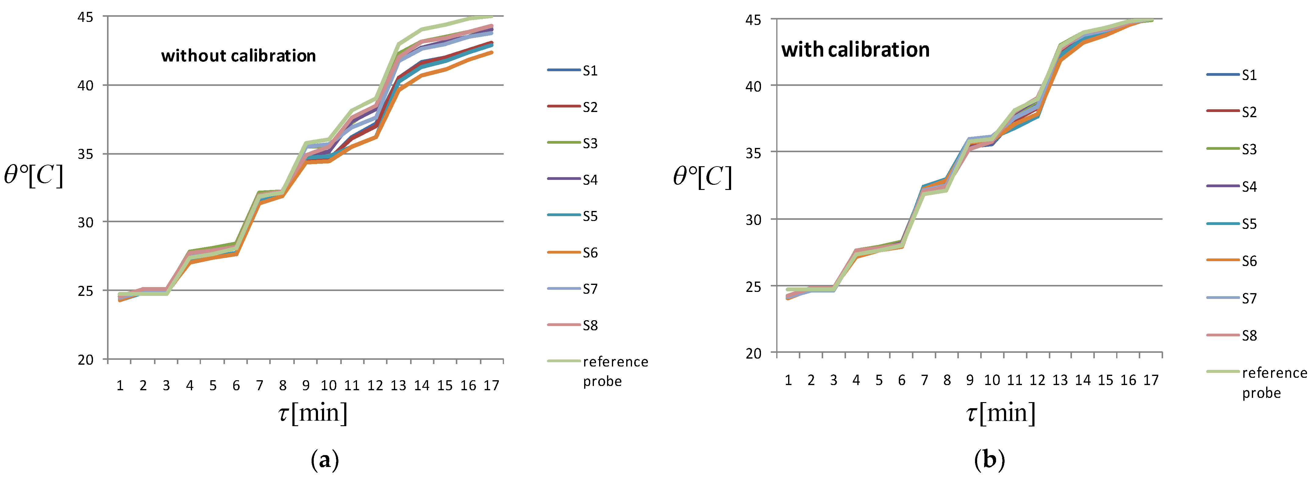
3.1. Calibration of the Advanced Thermal Manikin

The determination of the equivalent temperature is based on the equations of heat transfer by convection and radiation of the dressed occupants. The conduction heat exchange is considered to be reduced in comparison with that exchanged by convection and radiation
R = h r ( t s k t r ) [ W / m 2 ] , C = h c ( t s k t a ) [ W / m 2 ]
R—the density of thermal flux exchanged by radiation between the body and the environment; C—thermal flux density changed by convection between the body and the environment; hr—radiative heat transfer coefficient [W/m2K]; hc—convective heat transfer coefficient [W/m2K]; tsk—skin temperature [°C]; tr—average radiation temperature [°C]; ta —indoor air temperature [°C]. In the practical approach for assessing the equivalent temperature we use the following relationship:
t e q = t s Q t c a l [ ° C ]
ts—surface temperature; teq—temperature of the standard medium; Q—heat loss by convection and radiation under the real test conditions; tcal—is the combined coefficient of heat transfer by convection and radiation
Q = R + C
The advantage of using this index is the possibility of both a global assessment by establishing an equivalent temperature at the body level and a local assessment of comfort at the level of the area of the body.
This prototype is calibrated periodically in a climatic chamber in order to find the relationship between the ambient temperature and the heat loss. The climatic chamber (3.6 m × 3.6 m × 2.5 m) has the temperature controlled for the walls, floor, ceiling, and door, which allow the temperature to be adjusted. At the same time, the climatic chamber an advanced ventilation system with multiple inlets and outlets that is capable of providing several ventilation strategies can be operated. To measure the air temperature in the climatic chamber and the surface temperatures of the walls, PT100 sensors that were connected to a data acquisition logger were used. The temperature sensors were calibrated from 0 °C to 34 °C, with a precision of 0.2 °C. A temperature sensor is positioned on each wall, and six sensors are placed in the proximity of the thermal manikin and are distributed along the whole height of the room. The distance between these six sensors is 35 cm in order to obtain the vertical gradient temperature. The relative humidity is monitored as well. The mean air velocity of the airflow inside the test cell was recorded as 0.1 m/s n all calibration campaigns using an omnidirectional air velocity sensor (draught probe from a Comfort Sense system). During the calibration, the air temperature inside the climatic chamber is maintained at 24 °C, demonstrating the same value as the mean radiant temperature of the walls. The results from one calibration campaign are presented.
For the first calibration, the thermal manikin was placed in a seated position in the center of the climatic chamber with a uniform surface temperature of 34 °C. For the second calibration, the anatomic distribution of temperature was considered. The values of the heat transfer coefficients trough convection (hc) and radiation (hr) were calculated for the current thermal manikin (see Table 2) and were found to be similar to the results from the literature (see Table 3 and Table 4). Additionally, the deviations between the convective and radiative heat transfer coefficients compared those from the literature are presented in Table 5 and Table 6.

3.2. Measuring the Equivalent Temperature

As mentioned previously, the equivalent temperature is a quantitative assessment of the conditions for physical heat balance. Thus, to determine the equivalent temperature, it is necessary to measure the total heat flux of one or more zones, each of which have a specific surface temperature of a constant value. The set point of this value is chosen to be similar to the typical values of various human body zones. An indication of the convective, radiative, and conductive type heat losses is given by the power consumption. It is important to note that these measurements and control are possible through the LabVIEW software. For each zone, the direct quantity that is measured is the power consumption or heat loss and the surface temperature. Through normalization to an interior climate, the heat loss can be converted to the equivalent temperature. The equivalent temperature of one segment is found through the measurement of the power consumption of the corresponding heated zone, thus constituting an indicator for the local thermal comfort. The electrical energy that is consumed by the thermostatic system is estimated through the generation of a calibration gradient between the PWM duty-cycle and the power calculated as a point by point mean of a single pulse period. The voltage difference on the patch was estimated using the measurements from the oscilloscope. Thus, the voltage difference is obtained at the leads of the whole circuit from which the voltage difference on the transistors must be subtracted. Using a TH5A current transducer, the current through each patch was measured, and this was converted into an equivalent temperature using the relation:
t e q = t r e g P S r e g h c a l
teq—equivalent temperature; treg—the mean temperature of surface portion determined with a sliding mean during a preset period of time; S—surface portion area of the manikin; P—mean power consumption determined using a sliding mean during a preset period of time; hcal—convection coefficient determination using the preceding relationship for constant ambiental temperature (teq) of 24 °C and manikin’s surface temperature controlled at 34 °C [46,52].
If we compare to the traditional measurement methods through which we can estimate the global PMV, the advantage of the thermal manikin is that it can assess thermal comfort at a local scale and can predict local sensations through the use of the equivalent temperature or through a local PMV that is based on the equivalent temperature instead of the air temperature and the operative temperature [53]. Thermal manikins constitute a powerful assessment tool for the evaluation of the thermal comfort analysis both for lab conditions and for real case studies. Additionally, through the evaluation of the local values of equivalent temperatures for different manikin body parts, local discomfort can be investigated. This method of representing the equivalent temperature enables, for example, the evaluation of the uniformity of the environmental parameters. In Figure 16, we can see one example of our measurements of equivalent temperature distributions in the climatic chamber that were obtained with the thermal manikin (Suzi) data for five air flow rates in the climatic chamber, which are represented using the method defined by Nilsson [7,46,54] or by the standard EN ISO 14505/2 [8].
The map of the equivalent temperature seen as a perception of thermal sensation and thermal comfort is given by Figure 2 and Figure 22. Thermal sensations at different air flow rates are dependent on the teq obtained using the thermal manikin. A special utility of teq occurs in the case of asymmetric thermal conditions, such as in the case of a vehicle.

4. Conclusions

In order to assess comfort in enclosures with low temperature and radiation uniformity, the standard EN ISO14505/2 proposes the equivalent temperature method, which allows the furth use of complex measurement tools such as thermal manikins. In our opinion, the assessment of thermal environments with strong transient characteristics shall always be based on the measurement of the equivalent temperature, allowing both global and local estimations.
The indoor environment might be evaluated in terms of local effects for different areas of the human body. The local equivalent temperature shows us to what extent the parts of the body are in the area of acceptability in terms of heat loss. The equivalent temperature is a quantity that takes both the exchange of heat by convection and that by radiation between the human body and the environment into account. However, being a heat balance-based method, it does not take the subjective sensations that are perceived by the occupant into account, but in practice, it has been observed that there is a close connection between the thermal sensation that is felt by the occupant and the equivalent temperature.
Let us start by saying that teq measurement can be conducted with dedicated individual sensors for all of the intervening variables, e.g., thermal comfort meters with heated sensor, local discomfort meters, plane surface sensors, and thermal manikins. Of these, the usage of thermal manikins is considered the reference method with which other methods are compared. Significant differences were found in the values of equivalent temperatures arising from different methods in tests that were performed in uniform environments inside of a climatic chamber. These differences can be attributed to different characteristics of the measuring devices, such as size, geometry, posture, number and type of sensors, control method, etc. Nowadays, scientific research shows only rare solitary set-ups that are used to assess thermal comfort in vehicles that use the equivalent temperatures experimentally. These are either very expensive or are only suitable for punctual measurements. However, data acquisition at different locations in the interior space of a vehicle is highly desired, generating the need for cost-effective and accurate systems that are supposed to provide access to the local equivalent temperatures and further, especially if strong thermal gradients are present if the real ventilation systems are considered, to simulate the impact of heat exchange on the real occupants of buildings and vehicles as well.
The purpose of this paper was to present a recently designed and created thermal manikin with 79 superficial zones with independent neuro-fuzzy temperature regulation in detail. Both the component parts of the manikin and the acceptance strategy for this powerful measurement instrument were discussed.
Following papers will integrate with model with one of the respiratory systems that were developed in our laboratory in order to combine the interactions of the respiratory flows with the functioning of the thermal manikin.

Author Contributions

Conceptualization, I.N., I.U., D.D.I.-G. and P.A.D.; methodology, I.N., I.U., D.D.I.-G., P.A.D. and C.V.C.; software, I.U., D.D.I.-G., A.T. and D.E.; validation, I.U., D.D.I.-G. and P.A.D.; formal analysis, F.I.B.; resources, I.N., I.U. and D.D.I.-G.; data curation, P.A.D.; writing—original draft preparation, P.A.D., I.N. and I.U., writing—review and editing, F.I.B., M.S., D.E. and C.V.C.; funding acquisition, I.N. All authors have read and agreed to the published version of the manuscript.

Funding

This work was supported by a grant from the Romanian Space Agency ROSA—QUEST: Advanced air diffusion system of the crew quarters for the ISS and deep space habitation systems, STAR-CDI-C3-2016-577, and by the grants from the Romanian Ministry of Education and Research, CCCDI-UEFISCDI, EQUATOR: Advanced strategies for high performance indoor Environmental QUAliTy in Operating Rooms—PN-II-PT-PCCA-2011-3.2-0512 and XTREME: Innovative system to extend the range of electric vehicle at improved thermal comfort, project number PN-III-P2-2.1-PED-2019-4249, within PNCDI III.

Institutional Review Board Statement

Not applicable.

Informed Consent Statement

Not applicable.

Data Availability Statement

Not applicable.

Conflicts of Interest

The authors declare no conflict of interest.

References

  1. Santamouris, M.; Asimakopoulos, D. Passive Cooling of Buildings, 1st ed.; James & James Science Publishers Ltd.: London, UK, 1996. [Google Scholar]
  2. ASHRAE. Thermal Environmental Conditions for Human Occupancy; ANSI/ASHRAE Standard 55-2004; American Society of Heating, Refrigerating and Air-Conditioning Engineers: Atlanta, GA, USA, 2004. [Google Scholar]
  3. Hensen, J.L.M. Literature review on thermal comfort in transient conditions. Build. Environ. 1990, 25, 309–316. [Google Scholar] [CrossRef]
  4. ISO 7730; Ergonomics of the Thermal Environment—Analytical Determination and Interpretation of Thermal Comfort Using Calculation of the Pmv and Ppd Indices and Local Thermal Comfort Criteria. 3rd ed. International Organization for Standardization (ISO): Geneva, Switzerland, 2005.
  5. Fanger, P.O. (Ed.) Thermal Comfort-Analysis and Applications in Environmental Engineering; Mcgraw-Hill: New York, NY, USA, 1970. [Google Scholar]
  6. Djongyang, N.; Tchinda, R.; Njomo, D. Thermal comfort: A review paper. Renew. Sustain. Energy Rev. 2010, 14, 2626–2640. [Google Scholar] [CrossRef]
  7. Nilsson, H.O. Thermal comfort evaluation with virtual manikin methods. Build. Environ. 2007, 42, 4000–4005. [Google Scholar] [CrossRef]
  8. ISO 14505-3:2006; Ergonomics of the thermal Environment-Evaluation of Thermal Environments in Vehicles Part 2: Determination of Equivalent Temperature. International Organization for Standardization (ISO): Geneva, Switzerland, 2006.
  9. Nilsson, H.O. Comfort Climate Evaluation with Thermal Manikin Methods and Computer Simulation Models, 3rd ed.; National Institute for Working Life: Stockholm, Sweden, 2004; p. 37. [Google Scholar]
  10. Madsen, T.O.B.K.N. Comparison between operative and equivalent temperature under typical indoor conditions. ASHRAE Trans. 1984, 90, 1077–1090. [Google Scholar]
  11. Nilsson, H.; Holmér, I.; Holmberg, S.; Sandberg, M. Thermal climate assessment in office environment—CFD calculations and thermal manikin measurements. In Proceedings of the International Conference on Air Distribution in Room, Roomvent 2000—Reading, Reading, UK, 9–12 July 2000; pp. 90–95. [Google Scholar]
  12. Nilsson, H.O.; Holmér, I. Definitions and Measurements of Equivalent Temperature, European Commission Cost Contract no smt4-ct95-2017 Development of Standard Test Methods for Evaluation of Thermal Climate in Vehicles; Department of Technology and Built Environment University of Gävle: Gävle, Sweden, 2002. [Google Scholar]
  13. Baron, J. Thinking and Deciding; Cambridge University Press: Cambridge, UK, 2008; Volume 4. [Google Scholar]
  14. Baron, J. Against Bioethics; MIT Press: Cambridge, MA, USA, 2006. [Google Scholar]
  15. Baron, J. Norm-endorsement utilitarianism and the nature of utility. Econ. Philos. 1996, 12, 165–182. [Google Scholar] [CrossRef]
  16. Burke, R.; Rugh, J.; Farrington, R. ADAM—The Advanced Automotive Manikin. In Proceedings of the International Meeting on Thermal Manikins and Modelling, Strasbourg, France, 29–30 September 2003. [Google Scholar]
  17. Lebbin, P.; Hosni, M.; Gielda, T. Design and manufacturing of two thermal observation manikins for automobile applications. In Proceedings of the International Meeting on Thermal Manikins and Modelling, Strasbourg, France, 29–30 September 2003. [Google Scholar]
  18. Danca, P.; Nastase, I.; Bode, F.; Croitoru, C.; Dogeanu, A.; Meslem, A. Evaluation of the thermal comfort for its occupants inside a vehicle during summer. In IOP Conference Series: Materials Science and Engineering; IOP Publishing: Bristol, UK, 2019; Volume 595, p. 012027. [Google Scholar]
  19. Danca, P.; Bode, F.; Dogeanu, A.; Croitoru, C.; Sandu, M.; Meslem, A.; Nastase, I. Experimental study of thermal comfort in a vehicle cabin during the summer season. E3S Web Conf. 2019, 111, 01048. [Google Scholar] [CrossRef] [Green Version]
  20. Dogeanu, A.; Iatan, A.; Croitoru, C.; Nastase, I. Conception of a real human shaped thermal manikin for comfort assesment. In PhD & DLA Symposium; University of Pecs: Pesc, Hungary, 2012. [Google Scholar]
  21. Dogeanu, A.; Florin, B.; Iatan, A.; Croitoru, C.; Nastase, I. Conception of a simplified seated thermal manikin for CFD validation purposes. Rom. J. Civ. Eng. 2013, 5, 27. [Google Scholar]
  22. Gao, N.P.; Zhang, H.; Niu, J.L. Investigating indoor air quality and thermal comfort using a numerical thermal manikin. Indoor Built Environ. 2007, 16, 7–17. [Google Scholar] [CrossRef]
  23. Croitoru, C.; Nastase, I.; Bode, F.; Cojocaru, G. Assessment of virtual thermal manikins for thermal comfort numerical studies. Verification and validation. E3S Web Conf. 2019, 111, 02018. [Google Scholar] [CrossRef]
  24. Tacutu, L.; Nastase, I.; Bode, F.; Dogeanu, A.; Croitoru, C. Interaction between a local and a general ventilation system for an operating room with patient. In Proceedings of the 2019 International Conference on Energy and Environment (CIEM), Timisoara, Romania, 17–18 October 2019; pp. 348–353. [Google Scholar]
  25. Bode, F.; Tacutu, L.; Croitoru, C.; Nastase, I. Numerical and experimental study for the development of an advanced model of an operating room with surgeons and patient. In Proceedings of the 2017 International Conference on ENERGY and ENVIRONMENT (CIEM), Bucharest, Romania, 19–20 October 2017; pp. 447–451. [Google Scholar]
  26. Lee, Y.Y.; Md Din, M.F.; Noor, Z.Z.; Iwao, K.; Mat Taib, S.; Singh, L.; Abd Khalid, N.H.; Anting, N.; Aminudin, E. Surrogate human sensor for human skin surface temperature measurement in evaluating the impacts of thermal behaviour at outdoor environment. Measurement 2018, 118, 61–72. [Google Scholar] [CrossRef]
  27. Shi, S.; Li, Y.; Zhao, B. Deposition velocity of fine and ultrafine particles onto manikin surfaces in indoor environment of different facial air speeds. Build. Environ. 2014, 81, 388–395. [Google Scholar] [CrossRef]
  28. Holmér, I. Thermal manikin history and applications. Eur. J. Appl. Physiol. 2004, 92, 614–618. [Google Scholar] [CrossRef]
  29. Nayak, R.; Houshyar, S. 7—Comparison of manikin tests with wearer trials. In Manikins for Textile Evaluation; Woodhead Publishing: Sawston, UK, 2017; pp. 159–171. [Google Scholar] [CrossRef]
  30. Jambunathan, K.; Lai, E.; Moss, M.A.; Button, B.L. A review of heat transfer data for single circular jet impingement. Int. J. Heat Fluid Flow 1992, 13, 106–115. [Google Scholar] [CrossRef]
  31. Ursu, I.; Guţă, D.; Croitoru, C.; Danca, P.; Nastase, I. Advanced Thermal Manikin Prototype with Neuro-fuzzy Control System. In Proceedings of the COBEE 2018, Melbourne, Australia, 5–9 February 2018. [Google Scholar]
  32. Alahmer, A.; Mayyas, A.; Mayyas, A.A.; Omar, M.A.; Shan, D. Vehicular thermal comfort models; a comprehensive review. IAppl. Therm. Eng. 2011, 31, 995–1002. [Google Scholar] [CrossRef]
  33. Sakoi, T.; Tsuzuki, K.; Kato, S.; Ooka, R.; Song, D.; Zhu, S. Thermal comfort, skin temperature distribution, and sensible heat loss distribution in the sitting posture in various asymmetric radiant fields. Build. Environ. 2007, 42, 3984–3999. [Google Scholar] [CrossRef]
  34. Angel, D.; Cristiana, C.; Ilinca, N.; Mihnea, S.; Florin, B. Comfort evaluation using a thermal manikin. Comparison to subjective perception. In Proceedings of the SGEM2016 Conference, Albena, Bulgaria, 30 June–6 July 2016. [Google Scholar]
  35. Croitoru, C.; Nastase, I.; Voicu, I.; Meslem, A.; Sandu, M. Thermal Evaluation of an Innovative Type of Unglazed Solar Collector for Air Preheating. Energy Procedia 2016, 85, 149–155. [Google Scholar] [CrossRef]
  36. Halanay, A.; Ursu, I. Stability of equilibria of some switched nonlinear systems with applications to control synthesis for electrohydraulic servomechanisms. IMA J. Appl. Math. 2009, 74, 361–373. [Google Scholar] [CrossRef]
  37. Ouhimi, P.; Lechartier, T.; Danca, P.; Fabian, C. Thermal comfort evaluation inside vehicles with classical indices—Experimental approach. Rom. J. Civ. Eng. 2016, 7, 178. [Google Scholar]
  38. Vartires, A.; Dogeanu, A.; Danca, P. The human thermal comfort evaliation inside the passenger compartment. In Proceedings of the 15th International Multidisciplinary Scientific Geoconference, Albena, Bulgaria, 18–24 June 2015; pp. 1113–1120. [Google Scholar]
  39. Croitoru, C. Studii Teoretice și Experimentale Referitoare la Influenţa Turbulenţei Aerului din Încăperile Climatizate Asupra Confortului Termic. Ph.D. Thesis, Technical University of Civil Engineering of Bucharest, București, Romania, 2011. [Google Scholar]
  40. Operating Instructions—Lauda Eco silver—Heating and Cooling Thermostats with Control Head Silver. Available online: http://interlab.lt/download/ECO_Silver_instruction_manual.pdf.7559e65ad7b1afacdfbac0d98e4009f1 (accessed on 15 September 2021).
  41. Gardon, R.; Akfirat, J.C. The role of turbulence in determining the heat-transfer characteristics of impinging jets. Int. J. Heat Mass Transf. 1965, 8, 1261–1272. [Google Scholar] [CrossRef]
  42. Ioan, U.; Felicia, U.; Lucian, I. Neuro-fuzzy synthesis of flight control electrohydraulic servo. Aircr. Eng. Aerosp. Technol. 2001, 73, 465–472. [Google Scholar] [CrossRef]
  43. Ursu, I.; Tecuceanu, G.; Toader, A.; Calinoiu, C. Switching neuro-fuzzy control with antisaturating logic. Experimental results for hydrostatic servoactuators. Proc. Rom. Acad. Ser. A Math. Phys. Tech. Sci. Inf. Sci. 2011, 12, 231–238. [Google Scholar]
  44. Ursu, I.; Ursu, F. Airplane ABS control synthesis using fuzzy logic. J. Intell. Fuzzy Syst. 2005, 16, 23–32. [Google Scholar]
  45. Wang, L.X. Combining mathematical model and heuristics into controllers: An adaptive fuzzy control approach. In Proceedings of the 1994 33rd IEEE Conference on Decision and Control, Lake Buena Vista, FL, USA, 14–16 December 1994; Volume 4124, pp. 4122–4127. [Google Scholar]
  46. Quintela, D.; Gaspar, A.; Borges, C. Analysis of sensible heat exchanges from a thermal manikin. Eur. J. Appl. Physiol. 2004, 92, 663–668. [Google Scholar] [CrossRef]
  47. de Dear, R.J.; Arens, E.; Hui, Z.; Oguro, M. Convective and radiative heat transfer coefficients for individual human body segments. Int. J. Biometeorol. 1997, 40, 141–156. [Google Scholar] [CrossRef] [Green Version]
  48. Oliveira, A.V.M.; Gaspar, A.R.; Francisco, S.C.; Quintela, D.A. Convective heat transfer from a nude body under calm conditions: Assessment of the effects of walking with a thermal manikin. Int. J. Biometeorol. 2012, 56, 319–332. [Google Scholar] [CrossRef] [PubMed]
  49. Oliveira, A.V.M.; Gaspar, A.R.; Francisco, S.C.; Quintela, D.A. Analysis of natural and forced convection heat losses from a thermal manikin: Comparative assessment of the static and dynamic postures. J. Wind Eng. Ind. Aerodyn. 2014, 132, 66–76. [Google Scholar] [CrossRef]
  50. Fojtlín, M.; Fišer, J.; Jícha, M. Determination of convective and radiative heat transfer coefficients using 34-zones thermal manikin: Uncertainty and reproducibility evaluation. Exp. Therm. Fluid Sci. 2016, 77, 257–264. [Google Scholar] [CrossRef]
  51. Nilsson, H.; Holmér, I.; Bohm, M.; Norén, O. Equivalent temperature and thermal sensation—Comparison with subjective responses. In Proceedings of the Comfort in the Automotive Industry—Recent Development and Achievements; IOP Publishing: Bologna, Italy, 1997; pp. 157–162. [Google Scholar]
  52. Danca, P.A. Ventilation Strategies for Improving the Indoor Environment Quality in Vehicles. Ph.D. Thesis, Technical University of Civil Engineering of Bucharest, București, Romania, University of Rennes 1, Rennes, France, 2018. [Google Scholar]
  53. Wang, L.-X. Combining mathematical model and heuristics into controllers: An adaptive fuzzy control approach. Fuzzy Sets Syst. 1997, 89, 151–156. [Google Scholar] [CrossRef]
  54. Nastase, I.; Croitoru, C.; Lungu, C. A Questioning of the Thermal Sensation Vote Index Based on Questionnaire Survey for Real Working Environments. Energy Procedia 2016, 85, 366–374. [Google Scholar] [CrossRef] [Green Version]
Figure 1. Equivalent temperature definition based on [9].
Applsci 12 01826 g001
Figure 2. Comfort zones based on measured teq values in terms of subjective perception of conditions by vehicle occupants (after [8]): (a) summer case, (b)winter case.
Applsci 12 01826 g002
Figure 3. Set-ups for the measurement of teq as described in EN ISO 14505/2 after [8]; several discrete heated sensors mounted on a human-shaped dummy or a real person (a) or ellipsoid sensors mounted on a rig simulating a human body (b) are used.
Applsci 12 01826 g003
Figure 4. Two possible versions of manikins, as per EN ISO 14505/2—after [8]: (a) thermal manikin 33 zones, (b) thermal manikin 16 zones.
Applsci 12 01826 g004
Figure 5. Hardware development stages of the thermal manikin: (a) manufacturing patrons for the heating element (HE) disposal; (b) manufacturing the heating insulation under the thermal patches, (c) inserting the HE; (d) electrical circuits.
Applsci 12 01826 g005
Figure 6. Testing the (a) bottom and (b) the upper body parts; (c) HE embedded in silicon; (d) various geometries of the HE.
Applsci 12 01826 g006aApplsci 12 01826 g006b
Figure 7. The distribution of the HE on the individually controlled anatomical body parts (red patches refers to the respective opposite side of the manikin): (a) front view, (b) back view.
Applsci 12 01826 g007
Figure 8. (a) TSic T501 sensors used to measure and control part of the thermal manikin. (b) Thermostatic Lauda Eco water bath with Lauda Eco Silver immersion thermostat—Photographs taken during calibration campaigns for the TSic sensors.
Applsci 12 01826 g008
Figure 9. Variation in the resistance of several connected patches with the global temperature of the patch that was obtained after thermostatic bath essays.
Applsci 12 01826 g009
Figure 10. Distribution of the TSic T501 temperature sensors on the patches: (a) temperature sensors, (b,c) example of positions of the sensors on the patches.
Applsci 12 01826 g010
Figure 11. Response at thermal solicitations over time of TSic TO92 sensors: (a) without calibration, (b) with calibration.
Applsci 12 01826 g011
Figure 12. Multiplexer simplified circuit diagram.
Applsci 12 01826 g012
Figure 13. The basic system architecture of the manikin.
Applsci 12 01826 g013
Figure 14. The thermostatic system architecture.
Applsci 12 01826 g014
Figure 15. (a) Power supplies used for the manikin A—main power supply used for the heating patches; B—power supply used for myRIO boards; C—power supply used for sbRIO boards; D—computer used for manikin control and monitorization; (b) control system diagram for one control channel.
Applsci 12 01826 g015
Figure 16. (a) Schema of elementary perceptron; (b) singleton membership function for scaled fuzzy control u f .
Applsci 12 01826 g016
Figure 17. (a) Scaled variables y 1 , y 2 and (b) l 2 ( y 1 ) with their membership functions.
Applsci 12 01826 g017
Figure 18. Temperature variation: unsteady and steady regime.
Applsci 12 01826 g018
Figure 19. Tests for the temperature control of the thermal manikin using a regular fan (left). The behavior of thermoregulation system with neuro-fuzzy control when two zones (arm and forearm) are cooled with ambient temperature and at 0.8 m/s (right) (up—temperature, down—current consumption).
Applsci 12 01826 g019
Figure 20. User interface allowing the recording of the surface temperature for each segment and to control output for energy consumption.
Applsci 12 01826 g020
Figure 21. User interface for monitoring the equivalent temperature.
Applsci 12 01826 g021
Figure 22. teq distributions given by the thermal manikin data using various air flow rates in the climatic chamber using conditions described in [54].
Applsci 12 01826 g022
Table 1. Standardized values of the temperatures recommended to be maintained on the segments of thermal manikins [8].
Body RegionsRight FootRight LegRight ThighLeft FootLeft LegLeft ThighRight HandRight ArmRight Upper ArmLeft HandLeft ArmLeft Upper ArmHeadPelvic RegionChestBack
Anatomic temperature distribution (°C)27272727272730303030303034323232
Uniform temperature distribution (°C)34343434343434343434343434343434
Table 2. Heat transfer coefficients for the thermal manikin in seating position.
TemperatureAnatomic Temperature DistributionUniform Temperature Distribution
Segmenthc (W/m2K)hr (W/m2K)hc (W/m2K)hr (W/m2K)
Head4.744.474.684.58
Torso4.764.533.062.41
Right thigh4.163.324.163.88
Right tibia3.062.115.125.49
Right foot4.684.374.224.30
Right forearm6.865.734.694.17
Right arm4.644.284.964.94
Right hand4.964.925.184.94
Left hand4.964.924.644.52
Left arm4.624.234.964.95
Left forearm6.835.666.836.44
Left thigh4.694.384.624.49
Left tibia2.912.834.745.32
Left foot5.125.234.644.52
Back5.876.754.764.69
Pelvis4.644.295.875.02
Table 3. Convective heat transfer coefficients from the literature for other manikins.
Manikin Name/Body PartMonika [47]Maria [48]Maria [49]Maria [50]Newton [51]Suzi
(Current Study)
hc (W/m2 °C)
Left foot4.24.44.64.46.04.6
Right foot4.24.54.74.46.34.2
Left leg4.03.53.33.44.54.7
Right leg4.03.83.53.94.55.1
Left thigh3.73.73.73.94.44.6
Right thigh3.73.53.93.94.34.2
Pelvic region2.82.82.62.84.45.9
Head3.74.74.54.33.24.7
Left hand4.54.94.15.3-4.6
Right hand4.54.34.24.1-5.2
Left arm3.84.13.63.74.15.0
Right arm3.810.33.83.64.05.0
Left upper arm3.43.03.13.24.26.8
Right upper arm3.42.73.33.43.94.7
Chest3.02.32.22.33.13.1
Back2.62.22.62.83.44.8
Table 4. Radiative heat transfer coefficients from the literature.
Manikin Name/Body PartMonika [46]Newton [51]Suzy (Current Study)
hr (W/m2 °C)
Left foot4.25.24.5
Right foot4.24.84.3
Left leg5.45.25.3
Right leg5.44.95.5
Left thigh4.63.84.5
Right thigh4.63.43.9
Pelvic region4.84.95.0
Head3.93.04.6
Left hand3.9-4.5
Right hand3.9-4.9
Left arm5.24.45.0
Right arm5.24.04.9
Left upper arm4.84.25.0
Right upper arm4.84.44.2
Chest3.44.42.4
Back4.65.84.7
Table 5. Convective heat transfer standard deviations—manikins from literature and the current prototype.
Manikin Name/Body PartMonika [46]Maria [48]Maria [49]Maria [50]Newton [51]Suzi
(Current Study)
hc (W/m2 °C)
Left foot9.48%4.41%0.86%5.17%29.31%12.17%
Right foot0.00%7.96%11.90%4.76%50.00%12.30%
Left leg15.61%25.26%30.38%28.27%5.06%17.02%
Right leg21.88%25.51%31.64%23.83%12.11%18.90%
Left thigh19.91%20.07%19.91%15.58%4.76%13.04%
Right thigh11.06%15.11%6.25%6.25%3.37%6.74%
Pelvic region52.30%52.73%55.71%52.30%25.04%39.83%
Head20.94%−0.23%3.85%8.12%31.62%10.99%
Left hand3.02%−6.00%11.64%14.22%-14.73%
Right hand13.46%16.70%19.23%21.15%-14.23%
Left arm23.39%17.18%27.42%25.40%17.34%19.00%
Right arm23.39%107.08%23.39%27.42%19.35%16.66%
Left upper arm50.22%55.36%54.61%53.15%38.51%41.91%
Right upper arm27.51%41.91%29.64%27.51%16.84%24.11%
Chest1.96%23.57%28.10%24.84%−1.31%13.97%
Back45.38%53.86%45.38%41.18%28.57%36.11%
Table 6. Radiative heat transfer deviations—manikins from literature and the current prototype.
Manikin Name/Body PartMonika [46]Newton [51]Suzy (Current Study)
Left foot7.08%−15.04%2.96%
Right foot2.33%−11.63%10.03%
Left leg1.50%2.26%33.02%
Right leg1.64%10.75%4.18%
Left thigh2.45%15.37%6.96%
Right thigh18.56%12.37%19.89%
Pelvic region4.38%2.39%7.23%
Head14.85%34.50%18.97%
Left hand13.72%-43.5%
Right hand20.41%-28.30%
Left arm5.05%11.11%4.15%
Right arm5.26%19.03%8.87%
Left upper arm3.03%15.15%11.66%
Right upper arm14.29%3.57%9.23%
Chest41.08%80.50%57.43%
Back1.92%22.60%4.67%
Publisher’s Note: MDPI stays neutral with regard to jurisdictional claims in published maps and institutional affiliations.

