Point Cloud Segmentation from iPhone-Based LiDAR Sensors Using the Tensor Feature

Featured Application

Point cloud segmentation, geometric feature extraction.

Abstract

With widely used LiDAR sensors included in consumer electronic devices, it is increasingly convenient to acquire point cloud data, but it is also difficult to segment the point cloud data obtained from these unprofessional LiDAR devices, due to their low accuracy and high noise. To address the issue, a point cloud segmentation method using the tensor feature is proposed. The normal vectors of the point cloud are computed based on initial tensor encoding, which are further encoded into the tensor of each point. Using the tensor from a nearby point, the tensor of the center point is aggregated in all dimensions from its neighborhood. Then, the tensor feature in the point is decomposed and different dimensional shape features are detected, and the point cloud dataset is segmented based on the clustering of the tensor feature. Using the point cloud dataset acquired from the iPhone-based LiDAR sensor, experiments were conducted, and results show that both normal vectors and tensors are computed, then the dataset is successfully segmented.

1. Introduction

The point cloud is a universal spatial information acquisition format and plays an important role in indoor and outdoor environment understanding [1]. In conventional point processing methods, the point cloud is usually defined as a spatial location, or as having textural information, and geometric features are computed from the unstructured point cloud; then, the data are segmented into different geometric or semantic structures for further processing, such as in object detection, classification, and scene understanding [2,3].

In recent years, with different kinds of Light Detection And Ranging (LiDAR) sensors included in consumer electronic devices, such as the iPhone or Kinect, it has become increasingly convenient to acquire point cloud data. However, it also raised many challenges for data processing, due to the low accuracy and high noise of the point cloud data collected by these unprofessional LiDAR devices. To address these issues, some processing techniques are applied [4,5,6,7,8], such as point cloud filter, denoising, normal computation, and resampling. Then features are extracted from the point cloud, and the data are segmented. To achieve this goal, many kinds of point cloud segmentation methods were proposed that extract the feature in different ways, including deep learning-based approaches.

To deal with these kinds of problems in a universal framework, this work proposes a tensor feature-based point cloud segmentation method, and the point cloud data in an actual scene is obtained from the iPhone LiDAR sensor. The contributions are as follows: (1) we conduct the theoretical derivation of the N-d tensor voting, which helps the high-dimensional normal vector computation and structure decomposition, and design the related algorithms (2) we compute the normal vectors from the noisy point cloud based on the two-step procedure of tensor encoding and aggregating; (3) we construct the tensor feature decomposing and clustering framework to segment the point cloud from the noisy scenes acquired by the iPhone LiDAR sensor, and make a comparison between several related methods.

The remainder of this paper is structured as follows. The next section gives an overview of works related to this paper. Section 3 provides a detailed description of the point cloud segmentation method based on the tensor feature, including normal vector computing, tensor aggregation, tensor feature decomposition, and point cloud clustering. Experiments are conducted and the results are discussed in Section 4, followed by the conclusions in Section 5.

2. Related Works

Based on the way features are computed, point cloud segmentation methods can be categorized into two types:

(1)

Point cloud segmentation based on the geometric feature extraction.

The geometric features of the point cloud can be computed directly from the unstructured, scattered data, using computation geometric theory, and geometric features [2,3,9], such as line features which represent the geometric frame line of the object structure, and flat features, which may be part of the continuous flat surfaces, are usually extracted. Since the edge is one of the most salient geometric features of the point cloud, different edge structures are usually computed. Then, the closed geometric features represented by the edges are detected, and the point cloud dataset is segmented based on the boundary of each segment [2,9,10]. It is simple and convenient for the computer to implement, but the data are usually over-segmented. Meanwhile, in regional growth-based methods [11,12], point cloud segmentation is started with a seed, which can be computed with the minimum curvature. Then the process is iteratively computed based on the curvature threshold values, and different point segments are generated. Compared with the regional growth-based method, seeds points are not needed in feature clustering-based methods, and the point cloud data are usually segmented based on the clustering of point features, such as the curvature, angle difference, and discreteness. No structures are predefined, and the point cloud dataset is just segmented based on the closeness of features, and the cluster methods can be the K-means cluster, fuzzy cluster, and mean shift cluster [13,14,15]. However, in the incomplete sample scene, a single object can be segmented into different groups. However, in geometric model fitting-based methods, the predefined geometric models, such as the box, sphere, and cylinder, are applied to the point cloud. Hough Transformation [16], Random Sample Consensus (referred to as RANSAC) [17], or KD-tree-based space division [18] are usually used to obtain the optimal fitting segmentation result. In addition, a more complex model fitting process is needed for the continuous smooth geometric structures. Hence, in the principal structure-based methods, the geometric features are computed using the neighborhood, based on Principal Component Analysis (PCA), and the geometric structures are represented by the eigenvalues [19]. Then, different kinds of structures are split into different categories by a supervised or unsupervised method, such as Support Vector Machine (SVM) [20]. Other kinds of geometric feature computation methods, including the tensor voting algorithm [21,22,23], where the geometric information is computed based on the tensor decomposition from the scattered point, share a similar feature computation principle with the point’s neighborhood. Geometric features are computed based on the spatial relations between the point and its neighborhood, without manual interactions of training operations. Due to the intuitive and direct representation of the geometric structures in the point cloud, the geometric feature-based point cloud segmentation method has been widely used for years. However, the computation result could be unstable and misjudged in situations where there are many noisy point samplings.

(2)

Point cloud segmentation based on the deep-learning neural network

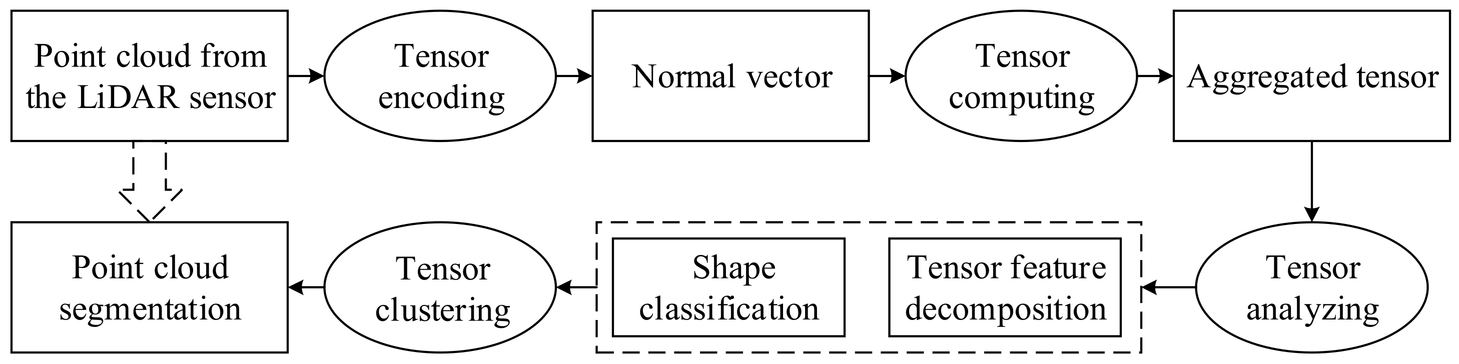
With the rapid development of graphics processing unit (GPU) parallel computing, deep-learning-based point cloud segmentation methods have been widely used and applied in many kinds of research. The point cloud dataset is separated into training, validation, and experimental datasets [4,5]. To deal with point cloud segmentation based on the 3D convolution neural network (CNN), the intuitive method is used to transform the 3D scattered point cloud into 2D images. Hence, in the multi-view CNN (MVCNN) [24]-based point cloud segmentation method, the point cloud in the training set is projected onto the 2D planes in a surrounding circle, then the neural network is trained and applied to semantic segmentation work. Though applied in 3D, the work is actually done with 2D processing. Some other similar works, such as group-view CNN (GVCNN) [25] and SqueezeSeg [26], actually use a similar technique. Another similar CNN-based method is 3D voxel-based point cloud segmentation [27], where the point cloud data are converted to spatially regularized voxels, then voxels are taken as 3D cubes and the 3D CNN-based deep-learning neural network is applied. These methods are adapted from the CNN of image processing, not directly designed for the scattered points; moreover, in the training dataset and validation dataset, the point cloud is labeled manually, and large amounts of the dataset are processed and input into the training program, which takes a long time to obtain the desired accuracy. In the first mentioned cloud segmentation method, PointNet [28] just takes the points as the input, and extracts the features of the data based on multi-layer perceptron (MLP), which can deal with the unstructured point cloud. Improvements have been made by PointNet++ [29] and other similar methods, with the neighborhood information accounted for. Another kind of point cloud segmentation method is the graph convolution-based method, which combines convolution with the graph structure. In the superpoints graph (SPG) [30], the point clouds are segmented and used as the super points of the graph, then split into each semantic group based on the graph convolution. However, the point data are still unstructured, and it is difficult to compute the convolution. To address the issue, PointCNN [31] applies the x transformation to the point cloud, and some other similar methods are proposed. These methods focus on both the segmentation and semantic labeling of the point cloud, and take the neighborhood and context into account, such as the scale. Some other improvements consider the attention mechanism of the neural network, such as in RandLA [32], or the feature encoding rules [33,34,35]. With the automatic fitting of the feature extracting and representing model, the point cloud can be quickly separated into different segments, even with the labels of each category. Nevertheless, the deep-learning neural network-based point cloud segmentation method is actually a statistical method, whose accuracy is limited by the training dataset and the result is affected by the pre-trained parameters. Moreover, if the kind of features that are not included in the training dataset or there are noise points in the input dataset, the result will become unstable.

To deal with the actual noisy dataset and acquire a stable geometric feature description from the input data, a point cloud segmentation method using the tensor feature is proposed in this paper, and the point cloud accessed on the iPhone-based LiDAR sensor is used. The proposed method belongs to geometric feature extraction-based point cloud segmentation, and several similar kinds of methods are experimented with and compared.

3. Methodology

Suppose the point p in the LiDAR point cloud consists of the coordinate, which can be shown as p(x,y,z). Based on tensor feature decomposition, the point cloud segmentation method assigns a label to each point p in difference subsets, and even gives them different geometric or semantic meanings. In this paper, the point cloud segmentation procedure is composed of the following steps:

(1)

normal vector computation based on the initial tensor encoding.

(2)

tensor aggregation from the tensor encoded with normal information.

(3)

tensor feature decomposition and shape classification by tensor analysis.

(4)

point cloud segmentation according to the tensor clustering.

The point cloud is collected from the LiDAR sensor and tensor features are encoded and assembled based on the tensor from the normal vector, then the point cloud dataset is segmented by the tensor feature clustering process, as shown in Figure 1.

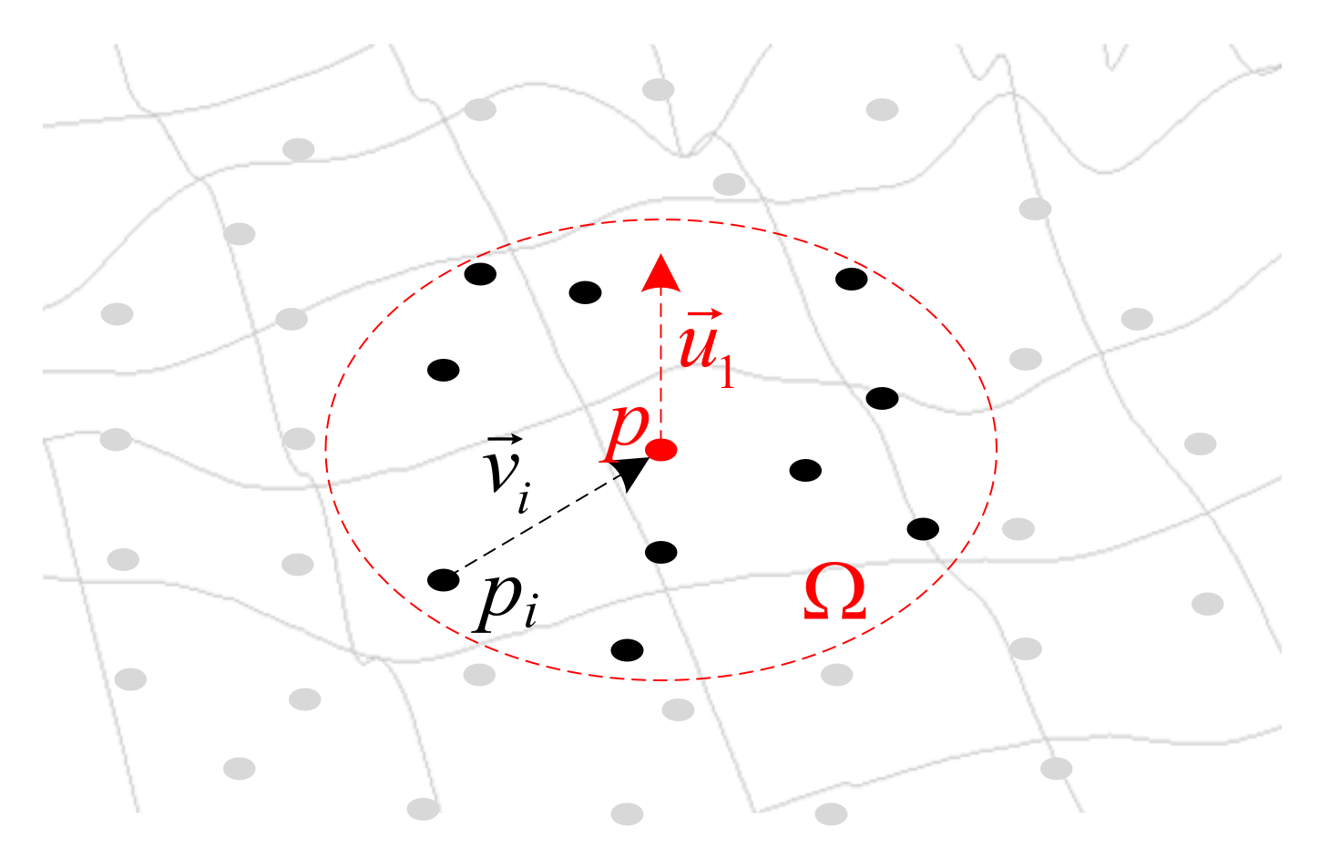
3.1. Normal Vector Computation Based on Initial Tensor Encoding

The normal vector of a point is the direction that is orthogonal to the direction of the structure. Suppose a d-dimensional geometric structure G, which is embedded in the N-dimensional space S with N basis vectors $\left({\overrightarrow{e}}_1,{\overrightarrow{e}}_2,\cdots ,{\overrightarrow{e}}_N\right)$. As depicted in the manifold theory, G is considered to be a manifold structure, with a d-dimensional normal subspace S_d and (N-d)-dimensional tangent subspace S_N-d, while the normal vector is considered to the basis vector $\left({\overrightarrow{e}}_1,{\overrightarrow{e}}_2,\cdots ,{\overrightarrow{e}}_d\right)$ of the normal subspace S_d, as shown in Equation (1). All kinds of structures of the point p of in G are encoded by the tensor of the normal subspace, ranging from 1-dimensional and 2-dimensional, to d-dimensional. In the 1-dimensional structure, the structure of G is considered to be a flat and continuous surface, and the normal space vector is considered to be a stick-shaped tensor. However, in the N-dimensional structure, the structure of G is considered to be a ball.

$$S=S_d+S_{N-d},s.t.,S_d={\displaystyle \sum _{n=1}^d{\overrightarrow{e}}_n}{\overrightarrow{e}}_n^T,S_{N-d}={\displaystyle \sum _{n=d+1}^N{\overrightarrow{e}}_n}{\overrightarrow{e}}_n^T$$

(1)

However, there is no normal information explicitly represented in the original point cloud, and the normal vector needs to be encoded from the ball tensor, where the dimension d = N. The initial tensor encoding is started from point p and its neighborhood $\mathrm{\Omega }$, which is consisted of k point except p:

(1)

arbitrarily pick up a point p_i from the neighborhood $\mathrm{\Omega }$, and compute the vector ${\overrightarrow{v}}_i$ from p_i to p, as shown in Equation (2), then normalize the vector ${\overrightarrow{v}}_i$ as ${\widehat{v}}_i$.

$${\overrightarrow{v}}_i=p-p_i,p_i\in \mathrm{\Omega }$$

(2)

(2)

compute the tensor T_i of tangent subspace S_N-d using the Kronecker delta of ${\widehat{v}}_i$ in Equation (2), and obtain the normal subspace S_d, based on Equation (1).

$$T_i={\rm I}-kron({\widehat{v}}_i,{\widehat{v}}_i^T)$$

(3)

As shown in Equation (3), the N-dimensional space S can be represented by the identity matrix I, since there is no preferred basis vector in the N-dimensional space.

(3)

gather the initial tensor from the neighborhood $\mathrm{\Omega }$, using the weight function w based on the vector ${\overrightarrow{v}}_i$, as shown in Equation (4). The weight w is a Gaussian function $w\left(s\right)=e^{-{\left(\frac{s}{\sigma }\right)}^2}$.

$$T={\displaystyle \sum _{i=1}^{i=k}w\left(‖{\overrightarrow{v}}_i‖\right)T_i}$$

(4)

(4)

calculate eigenvectors $\left({\overrightarrow{u}}_1,{\overrightarrow{u}}_{2,},\cdots ,{\overrightarrow{u}}_N\right)$ of the tensor T and choose the vector ${\overrightarrow{u}}_1$ (as shown in Figure 2) with the largest eigenvalues as the normal vector of point p. Here p can be treated as a point in the surface, and ${\overrightarrow{u}}_1$ is the 1-dimensional stick structure.

3.2. Tensor Aggregation Based on Normal Tensor Assembling

Since the geometric structure of the point p is unknown and the dimensional information is encoded in the tensor of each point, the tensor information at point p needs to be aggregated based on the normal tensor from its neighborhood, then the geometric information can be further judged by 1-dimensional, 2-dimensional, and N-dimensional structures, which will be discussed in Section 3.3.

(1)

tensor representation in each dimension using normal information

Using the normal vector computed in Section 3.1, the tensor field of each point p can be re-encoded based on the normal vector ${\overrightarrow{u}}_1$, as shown in Equation (5).

$$T_{}^{new}=kron\left({\overrightarrow{u}}_1^{},{\overrightarrow{u}}_1^T\right)$$

(5)

Then the tensor T^new is decomposed with eigenvectors $\left({\overrightarrow{\mu }}_1,{\overrightarrow{\mu }}_2,\cdots ,{\overrightarrow{\mu }}_N\right)$ and eigenvalues $\left({\varsigma }_1,{\varsigma }_2,\cdots ,{\varsigma }_N\right)$, where ${\varsigma }_1\ge {\varsigma }_2\ge \cdots \ge {\varsigma }_N$. The d-dimensional geometric structure D_d is assembled by the tensor of each eigenvector along with its dimensional saliency s, which is shown in Equation (6).

$$D_d={\displaystyle {\sum }_{i=1}^d{s}_i}\cdot kron\left({\overrightarrow{\mu }}_i^{},{\overrightarrow{\mu }}_i^T\right)$$

(6)

In Equation (6), the dimension saliency s_i is computed by eigenvalues, as shown in Equation (7).

$$s_i=\left\{\begin{array}{c}{\varsigma }_i-{\varsigma }_{i+1}\\ {\varsigma }_N\end{array}\right.\begin{array}{c},i<N\\ i=N\end{array}$$

(7)

(2)

geometric structure propagation based on tensor assembling

Suppose there is a point p_k in the neighborhood of point p, and the d-dimensional geometric structure D_d of the point p is going to be propagated to point p_k, as depicted in Figure 3, where N = 2.

As seen in the figure, the space S at p is decomposed into the normal vector v_n and tangent vector v_t, and the structure that was encoded by the normal vector is going to be propagated from p to p_k, along a curved path c. Since the normal vector is always orthogonal to the surface, both the normal vector v_n at p and that propagated to p_k (shown as v_k in Figure 3) share the same curvature, and intersect at the virtual center point o. The angle $\theta$ is the direction difference between the tangent vector v_t and the directly connected vector v that starts from point p to p_k, and can be computed based on Equation (8).

$$\theta =\mathrm{acos}\left(\mathrm{dot}\left(\frac{v_k}{‖v_k‖},v_t\right)\right)$$

(8)

Hence, other angle relations can be calculated using trigonometric function conversion formula. The normal v_nk vector at point p_k can be computed based on Equation (9).

$$v_{nk}=v_n\cos (2\theta )-v_t\sin (2\theta )$$

(9)

Using Equations (8) and (9), the tensor information propagated from point p to p_k, as shown in Equation (10).

$$T_{p->p_k}^d=\omega \left(r,\theta \right)\cdot kron\left(v_{nk},v_{nk}^T\right)$$

(10)

$\omega \left(r,\theta \right)=e^{{\left(\frac{r}{\sigma }\right)}^2}{\left(\cos \left(\theta \right)\right)}^4$ is the decaying function of the tensor information, and r is the distance between the two points which can be computed by $‖v‖$.

(3)

tensor aggregation of each dimensional structure from neighborhood

In the d-dimensional space S_d (as shown in Equation (1)), each dimensional geometric structure D_d, which is encoded by the base normal vector, should be projected to v_k based on the geometric angle relations. However, the process can be simplified based on the work of King [10], if the 1-dimensional basis normal vector ${\overrightarrow{v}}_{n,1}$ is chosen to be v_n, which is the projection of v_k to S_d (i.e., S_dv_k). In this case, the other dimensional basis vector will be orthogonal to v_k, and the angle $\theta$ will become 0, except that in 1-dimensional structures. Therefore, the tensor of T_d of geometric structure D_d, can be computed based on Equation (11).

$$T_p^i=T_{p->p_k}^{d=1}+T_{p->p_k}^{d>2}$$

(11)

$\theta$ will become 0 in $T_{p-p_k}^{d>2}$, and can be computed based on Equations (12) and (13).

$$T_{p->p_k}^{d=1}=\omega \left(r,\theta \right)\cdot kron(v_{nk}^{},v_{nk}^T)$$

(12)

$$T_{p->p_k}^{d>2}=\omega \left(r,0\right)\cdot \left(S_d^{}-kron\left(v_n,v_n^T\right)\right)$$

(13)

There are many structures encoded in tensor T^new, and each structure $T_p^i$ can be computed based on Equation (12) with its structure saliency s_i based on Equation (7). The aggregated tensor $T_p^{agg}$ from the point p in each dimensional i is shown in Equation (14).

$$T_p^{agg}={\displaystyle {\sum }_{i=1}^N{s}_i\cdot }{T}_p^i$$

(14)

Each of the points p in the neighborhood has a propagated tensor $T_{}^{agg}$, and the tensor aggregation result $T_{}^{agg}\left(p_k\right)$ of the point p_k by its neighborhood $\mathrm{\Omega }$ is shown in Equation (15).

$$T_{}^{agg}\left(p_k\right)={\displaystyle {\sum }_{p\in \mathrm{\Omega }}^{}{T}_p^{agg}}$$

(15)

3.3. Tensor Feature Decomposition and Shape Classification Based on Tensor Analyzing

As represented in Section 3.2, there are many kinds of geometric structures encoded in the tensor of each point, ranging from 1-dimensional, 2-dimensional, to N-dimensional structures. Through the eigenvalue decomposition, eigenvalues and eigenvectors are computed as follows:

(1)

eigenvalues $\left({\gamma }_1,{\gamma }_2,\cdots ,{\gamma }_N\right)$ with descending order, i.e., referred to as the intensity of each eigenvector;

(2)

eigenvectors $\left({\overrightarrow{\kappa }}_1,{\overrightarrow{\kappa }}_2,\cdots ,{\overrightarrow{\kappa }}_N\right)$, i.e., referred to as the dimension of the normal space, which is orthogonal to the manifold structures of G.

According to Equation (7), the d-dimensional geometric structure can be computed by the eigenvalues, along with the related eigenvectors. For example, as depicted in Figure 4, in the space S (N = 3):

(1)

the geometric structure with the 1-dimensional stick-shaped normal space, where there is just one normal vector (${\overrightarrow{\kappa }}_1$), tends to be the “surface”, and the geometric structure saliency $s_1={\gamma }_1-{\gamma }_2$;

(2)

the geometric structure with 2-dimensional surface-shaped normal space, where there are two normal vectors (${\overrightarrow{\kappa }}_1,{\overrightarrow{\kappa }}_2$), tends to be the “line” and the geometric structure saliency $s_2={\gamma }_2-{\gamma }_3$;

(3)

the geometric structure with 3-dimensional ball-shaped normal space, where there are three normal vectors (${\overrightarrow{\kappa }}_1,{\overrightarrow{\kappa }}_2,{\overrightarrow{\kappa }}_3$), tends to be the “point” and the geometric structure saliency $s_3={\gamma }_3$.

Using the above method, each point p is labeled with a shape descriptor $p\left(s_1,s_2,\cdots ,s_N\right)$, ranging from dimension 1 to dimension N. In addition, the normal vector can be further refined by using ${\overrightarrow{\kappa }}_1$, under the assumption that objects captured by the LiDAR point cloud have continuous surfaces, and the vector ${\overrightarrow{\kappa }}_1$ is the main vector that can be encoded into the 1-dimensional normal space.

3.4. Point Cloud Segmentation Based on Tensor Clustering

With the shape descriptor and refined normal vector computed as in Section 3.3, the point cloud data can be further processed in the following three aspects:

(1)

point feature filtering based on the ball tensor detecting

Since the 3D indoor/outdoor scene scanned by the LiDAR sensor is composed of objects with continuous surfaces, the point with a high geometric structure saliency of s_N (N = 3, in 3-dimensional space), which is presented as the ball tensor and turns out to be the scattered point, can be taken as noise point data. To deal with such cases, a threshold value ${\eta }_{point}$ to remove of the scattered noisy point cloud data, can be interactively set through a trivial operation, as shown in Equation (16).

$$P_{point}=\left\{p\left|s_N\in p\left(s_1,s_2,\cdots ,s_N\right)\&s_N>{\eta }_{noise}\right.\right\}$$

(16)

(2)

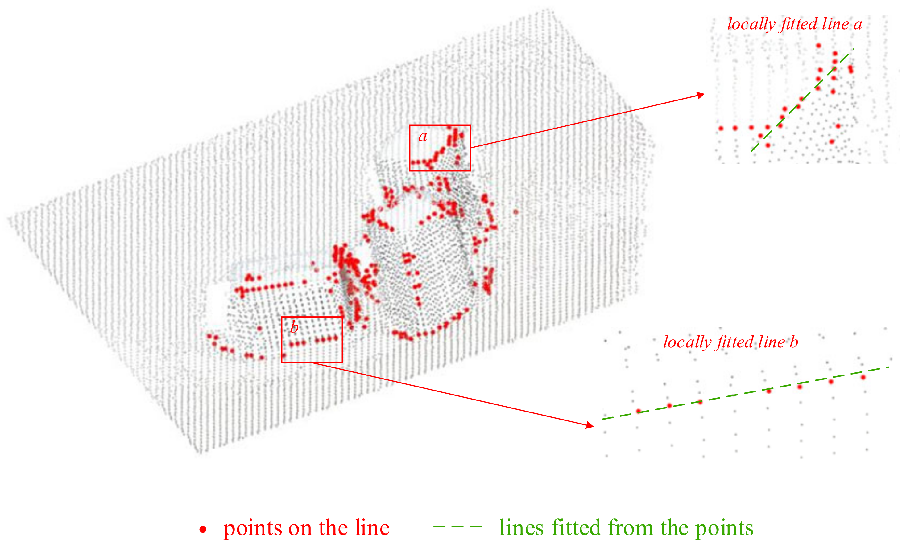
line feature extraction based on the line tensor classifying

Due to the noise and untrusted sampling of the point cloud, the saliency of the line geometric feature is affected to some extent. To extract the line feature, a threshold value ${\eta }_{line}$ is applied to each point, and points with saliency higher than ${\eta }_{line}$ are selected, as shown in Equation (17). The extracted points are actually in the buffer of the line feature, so the point in the extracted line feature is further simplified to become the line feature.

$$P_{line}=\left\{p\left|s_2\in p\left(s_1,s_2,\cdots ,s_N\right)\right.\&s_2>{\eta }_{line}\&Simplifying\right\}$$

(17)

(3)

surface feature segmentation based on the surface tensor clustering

Based on the regional growth method, the surface feature is segmented using the surface saliency s₁ and the refined normal vectors ${\overrightarrow{\kappa }}_1$ of each point. The detailed operations are as follows:

(1)

sort the surface saliency s₁ in descending order, and take the point with the largest saliency as the seed point p;

(2)

initialize the cluster set C and seed set E, push p into E, and search the neighborhood $\mathrm{\Omega }$ points of p using the searching radius r;

(3)

for each of the point p_i in the $\mathrm{\Omega }$, compute the angle difference $\theta \left({\kappa }_1^p,{\kappa }_1^{p_i}\right)$ between the normal vector of p and p_i. Push p_i to C if $\theta \left(p,p_i\right)<{\theta }_{surface}$, in addition, push p_i to Q if $s_1^{p_i}<{\eta }_{surface}$;

(4)

delete the current seed point p from Q, and repeat step 3 until there is no seed point in Q.

The point cloud segmentation result is the line feature and segmented surface features, while the point feature is filtered from the original point cloud data.

3.5. The Algorithm of the Point Cloud Segmentation Workflow

Based on the processing stages of tensor features, the algorithm of the point cloud segmentation workflow is composed of three main steps, including normal vector computation, tensor aggregation, and point segmentation, which are depicted in Algorithm 1.

Algorithm 1 The algorithm of the point cloud segmentation workflow

Point cloud Segmentation based on the Tensor Feature PSTF(P, r) INPUT: point cloud P, the searching distance for the neighborhood r, segmentation thresholds {${\eta }_{point}$,${\eta }_{line}$,${\eta }_{surface}$,${\theta }_{surface}$} OUTPUT: segmented point cloud sets PSeg //Stage 1: Normal vector computation based on initial tensor encoding FOREACH p in P   $\mathrm{\Omega }\left\{p_i|\Vert p-p_i\Vert \le r\right\}$ = GetNeighborhood(p, r);//get the neighborhood of p   [${\overrightarrow{v}}_i$$,{\widehat{v}}_i$]= ComputeVoteVector(p,pi$\in \mathrm{\Omega }$);//based on Equation (2)   T = VoteEncodingByNeighborhood(p, pi$\in \mathrm{\Omega }$, ${\widehat{v}}_i\in \mathrm{\Omega }$);//based on Equations (3) and (4)   ${\overrightarrow{u}}_1$ = GetOneDimStickVector(T);//based on Equation (1) END //Stage 2: Tensor aggregation based on normal tensor assembling FOREACH p in P   Tnew = ReEncoding(${\overrightarrow{u}}_1$);//based on Equation (5)   [$\overrightarrow{\mu },\varsigma$] = EigenDecomposition(Tnew);//get the decomposed eigenvectors and eigenvalues from the re-encoded tensor   $\mathrm{\Omega }\left\{p_k|\Vert p-p_k\Vert \le r\right\}$ = GetNeighborhood(p, r);//get the neighborhood of p    FOREACH d in N//structures in each dimension for point p     Dd = ComputeStructureTensor($\overrightarrow{\mu }$);//based on Equation (6)     si = ComouteSturctureSaliency($\varsigma$);//based on Equation (7)     [vn, vt, vk] = ComputeVector(p, pk$\in \mathrm{\Omega }$);//compute vectors for the voting     $\theta$ = ComputeAngleDifference(vt, vk);//based on Equation (8)     vnk = ComputePropergatedVector(vn, vt, $\theta$);//based on Equation (9)     $T_{p->p_k}^d$ = ComputeTensorFeature(vnk);//based on Equation (10)     $T_p^{i=d}$ = ComputeDDimensionalTensor($T_{p->p_k}^{d=1}$, $T_{p->p_k}^{d\ge 2}$, pk$\in \mathrm{\Omega }$);//based on Equations (11)–(13).   END   $T_p^{agg}$ = AggregateTensor(si, $T_p^i$);//based on Equation (14)   $T_{}^{agg}\left(p_k\in \mathrm{\Omega }\right)$ = PropagateTensor($T_p^{agg}$);//based on Equation (15) END //Stage 3: Tensor feature decomposition based on tensor analyzing [$\overrightarrow{\kappa },\gamma$] = EigenDecomposition(Tagg);//get the decomposed eigenvectors and eigenvalues from the aggregated tensor [s1,s2,…,sn] = ComputeGeometricDescriptor($\gamma$);//geometric structure decomposition //Stage 4: Point cloud segmentation based on tensor clustering Ppoint = PointFeatureFiltering(s,${\eta }_{point}$);//based on Equation (16) Ppoint = LineFeatureExtration(s,${\eta }_{line}$);//based on Equation (17) Psurface = SurfaceFeatureFiltering(s,${\eta }_{surface}$,${\theta }_{surface}$);//get the surface feature RETURN PSeg{Ppoint, Pline, Psurface}

4. Experiments and Discussions

This section focuses on the experiments with point cloud segmentation based on the method described in Section 3. There are two different experiments conducted based on the dataset acquired from the LiDAR sensor: the first experiment is to illustrate the detailed steps and information of the proposed method, while the second experiment is to validate the capability of the proposed method. In the first experiment, the point clouds are acquired from the iPhone-based LiDAR sensor, then normal vectors are computed based on the initially encoded tensor. The tensor at each point is re-encoded using normal information and aggregated from its neighborhood, followed by tensor feature decomposition and shape classification operations. Finally, the point cloud segmentation method is conducted using the clustering process, along with comparisons and a discussion.

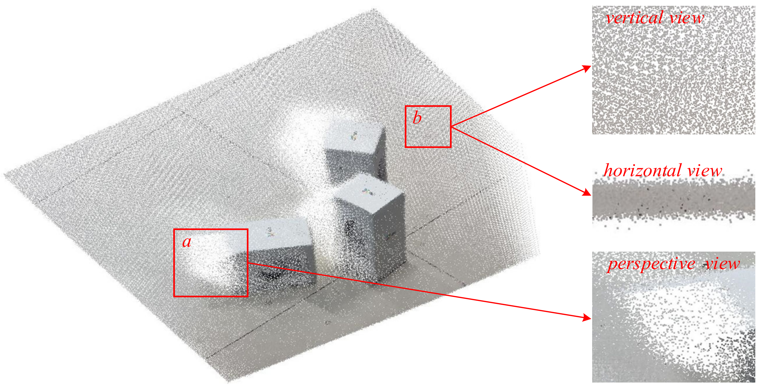
4.1. Datasets from the iPhone-Based LiDAR Sensor

In this paper, point cloud data are obtained from the LiDAR sensor included with the iPhone 12 Pro Max, which is a kind of consumer electronic device, as depicted in Figure 5. The LiDAR sensor is a solid-state device with a range of 5 m and low resolutions, and the point cloud data are obtained based on TOF (Time of Flight) technology.

In the first experiment, the dataset is in a small scene consisting of three cubes on the ground with an area of 1.49 m², and the point number is 15,599, as depicted in Figure 6. In addition, the dataset is affected by the noisy point cloud samplings by the LiDAR sensor. Hence, as the data quality index, the standard deviation (std.) is computed based on the distribution of the point cloud on a flat plane, which is acquired from the datasets with a flat area. In the dataset, the mean square error is 0.0018 m.

4.2. Normal Vector Computation and Refinement Based on the Tensor Feature Encoding

There are two steps for the normal vector computation, after setting the searching distance r at 0.3 m. First, normal vectors are computed from the scatted points using the initial tensor encoding, and the eigenvectors with the largest eigenvalues are used as the normal vector; secondly, the initially computed normal vectors are re-encoded into the tensor, and the normal vectors are re-computed and refined in a similar way to the first step.

As depicted in Figure 7, the normal vectors are computed using the parameter $\sigma$ = 0.1. Although it is a flat area the normal vectors are in a specific direction, there are many normal vectors with chaotic normal directions, which are caused by the noisy data samplings, as shown in Figure 7, enlarged view a. Hence, a refinement process is conducted, and the normal vectors are re-computed and refined. In the refined result, the direction of the normal vector becomes more regularized in the flat plane, compared with the first computed result.

4.3. Shape Description Using the Tensor Analyzing

The tensor at the point p is aggregated from its neighborhood with the normal information encoded, and the geometric structures in each dimension are propagated to p. After the tensor aggregation process, the tensor at each point is decomposed into 1-dimensional, 2-dimensional, and 3-dimensional geometric features, as depicted in Figure 8.

As seen in Figure 8, there are three types of geometric features in the dataset and each has related saliency figure. The saliency of points in Figure 8a are higher between the single objects, which can be taken as the noisy point samplings and filtered out from the dataset. However, the saliency of line in Figure 8b describes the framework of the geometric objects, which is higher than that of other points. In Figure 8c, the saliency of the surface is obviously higher on the ground, while not higher than that in the single objects, and this might be caused by the size of the neighborhood, since a larger neighborhood is set for noisy data samplings.

The line features of the dataset are extracted using the line saliency threshold value, then the line features are further shrunk to a single line, as depicted in Figure 9. The threshold value for the dataset is ${\eta }_{line}$ = 500, and the line features are extracted with a value higher than the threshold value.

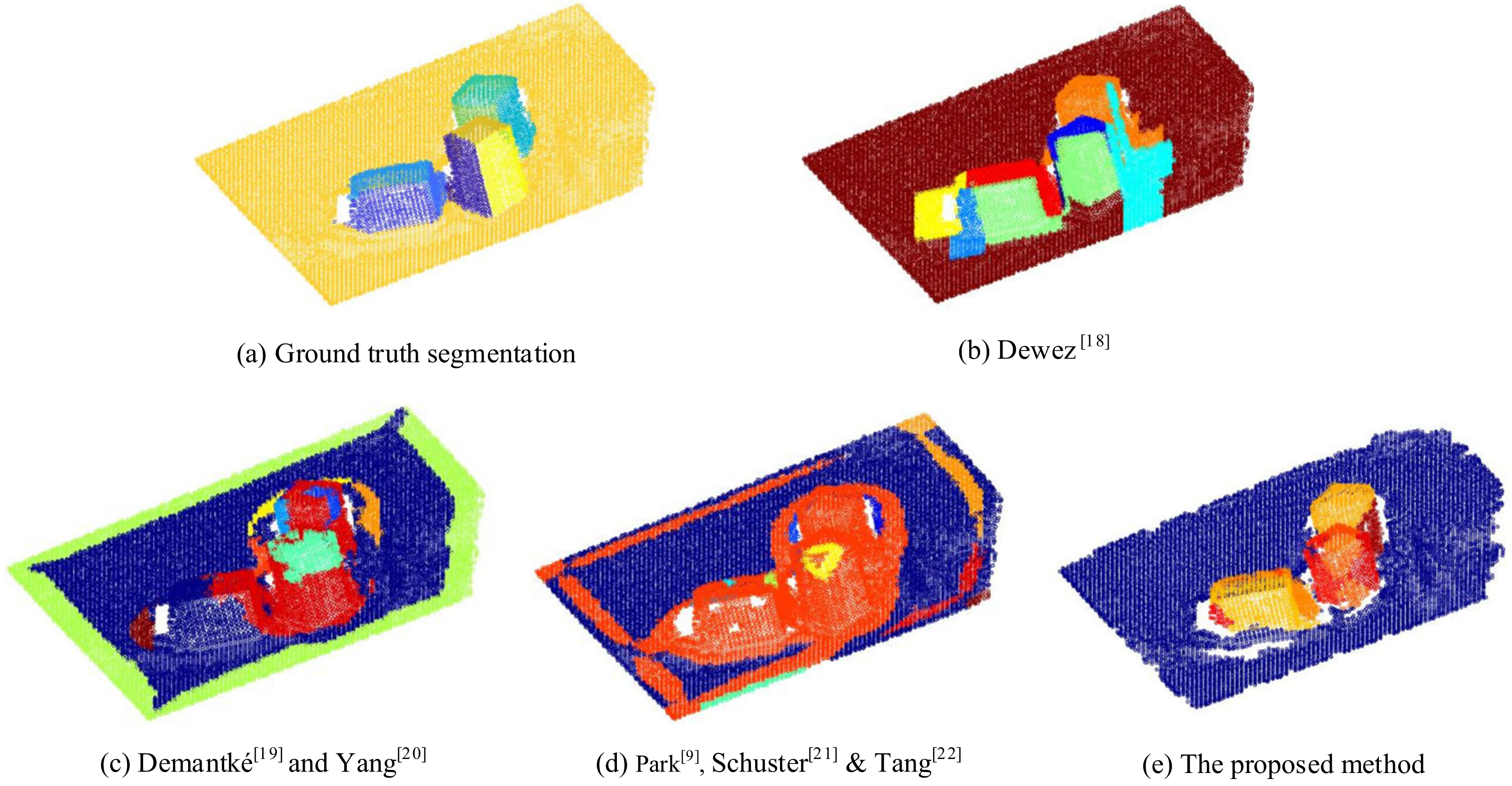
4.4. Point Cloud Segmentation Based on the Tensor Clustering

To remove the noisy point in the point cloud, the point with a point saliency higher than the threshold value ${\eta }_{point}$ = 100 is taken as the noise and is further removed from the dataset. Moreover, the point cloud datasets are segmented based on tensor clustering, using the regional growth of the surface saliency ${\eta }_{surface}$ = 110 and the related normal vectors. In the noisy point cloud datasets, a high angle threshold value is needed. Here, the angle threshold value for the normal vectors is set to ${\theta }_{surface}$= 10°, and any normal vector with an angle difference higher than that threshold value is considered to be a different surface. To verify the segmentation result of the proposed method, a comparison is made between the different geometric feature-based point cloud segmentation methods, as depicted in Figure 10, and the ground truth segmentation with ten parts is shown in Figure 10a.

Since the PCA method and the optimal searching distance are both applied in Demantké [19] and Yang [20], they are put into the same method group; moreover, a similar strategy to compute the tensor is applied in Park [9], Schuster [21], and Tang [22], and these three methods are also put into the same method group. Hence, as seen in Figure 10, KD-tree-based space division by Dewez [18], the PCA method by Demantké [19] and Yang [20], tensor voting by Park [9], Schuster [21], and Tang [22], and the proposed method are all experimented with, and the results of the point cloud in the dataset are compared. In Figure 10b, the dataset is segmented into 16 parts, using the automatically computed parameters {Max angle: 5°, Max relative distance: 1.0 m, Max distance: 0.1 m, Min points per facet: 10, Max edge length 0.00} by the algorithm. Since the searching distance r of the methods by Demantké [19] and Yang [20], Park [9], Schuster [21], and Tang [22] can be adaptively selected, set $r\in \left[0.1,0.3\right]$ m. As a result, the point cloud in Figure 10c is segmented into 12 parts, and in Figure 10d, the number of the segments is also 12 parts. However, in Figure 10e, the point cloud conducted by the proposed method is segmented into 17 parts. In the comparison, the point cloud segmented by the proposed method outperforms others, where the ground and different objects are successfully segmented, although the results are a little over-segmented due to the noisy point cloud samplings. Moreover, in the point cloud segmentation procedure, the noisy point cloud samplings acquired from the iPhone LiDAR sensor are successfully segmented into different parts. With the line saliency, the line features are extracted, and different surface segments are generated based on the surface saliency, after the denoising process based on the point saliency.

$$F_{score}=2\times \frac{precision\ast recall}{precision+recall}$$

(18)

As a quantified measure, F_score is a widely used accuracy index to measure the performance of the algorithm, as shown in Equation (18); hence, it is applied here to evaluate the accuracy of point segmentation results with different methods. Here, the precision of F_score is computed based on points in each segmented result and the number of points which truly belong to the related plane, and the recall is computed based on points in each segmented result and the number of the points in the related ground truth segments. To compute the detailed accuracy description, the precision, recall, and F_score of each segmentation result are computed based on the ground truth segmentation in Figure 11a.

The F_score for each part of the segmentation result is illustrated in Figure 11. As seen in the figure, the lighter (yellower) the color, the higher the F_score, while the darker (redder) the color, the lower the F_score. The ground part of the segmentation result in Figure 11a is lighter than that of the result in Figure 11b,c, but in other parts, the situation becomes complex: some parts of the image are darker in one method than in the same part of another, while in other parts this is not the case. However, compared with Figure 11d, the results become definite and clear: most of the parts are lighter than others and the results outperform others.

The statistics of precision, recall, F_score of each part in the segmentation result is further conducted, and the average values are computed and illustrated in

Table 1. The F_score computation results.

Different Methods	Average Precision	Average Recall	Average Fscore
Dewez [18]	0.6797	0.3104	0.2963
Demantké [19] and Yang [20]	0.8133	0.2414	0.2579
Park [9], Schuster [21] and Tang [22]	0.8779	0.0987	0.1359
The proposed method	0.8230	0.4250	0.4828

. Due to the diverse number of the segmentation results, the average values are calculated for each method.

As seen in Table 1, the average precision of the proposed method is 0.8230, which is a little lower than that of Park [9], Schuster [21], and Tang [22] with an average precision of 0.8133. However, the average recall of the proposed method is 0.4250, which is the highest in the comparison, and that of the Park [9], Schuster [21], and Tang [22] is 0.0987. Hence, the average F_scores for the proposed method by Dewez [18], Demantké [19] and Yang [20], Park [9], Schuster [21], and Tang [22], are 0.4828, 0.2963, 0.2579, and 0.1359, respectively. From the statistics, the proposed method overall performs better than the other methods, which is consistent with the result in Figure 11.

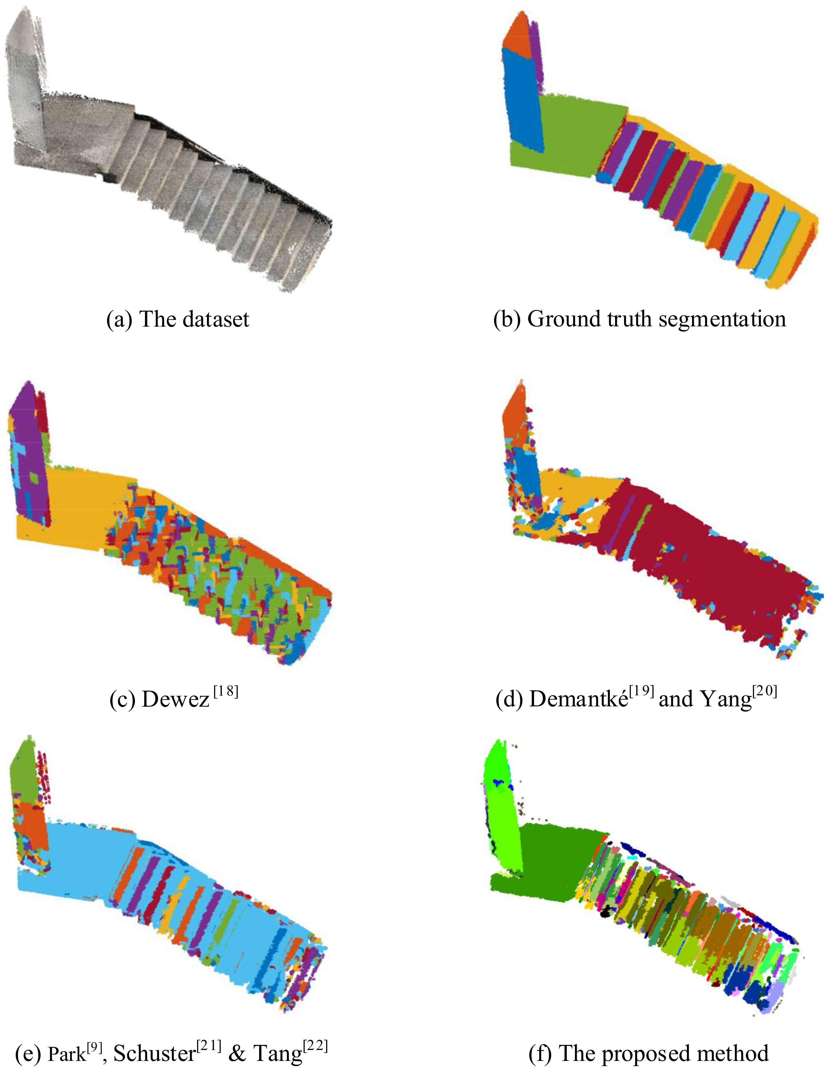
4.5. Point Cloud Segmentation for the Dataset in the Large Area

Since the main purpose of the method is to segment the point cloud into different plane structures, to verify the capability of the proposed point cloud segmentation method, the other dataset is obtained from the iPhone-based LiDAR sensor, in an area of 22.78 m², with 141,837 points, as depicted in Figure 12a. It is a stairway scene, and is divided into 31 parts in ground truth segmentation, as depicted in Figure 12b. The point cloud segmentation results of different methods are depicted from Figure 12c–f. In Figure 12c, the dataset is segmented into 295 parts, using the automatically computed parameter {Max angle: 10°, Max relative distance: 2.0 m, Max distance: 0.1 m, Min points per facet: 10, Max edge length 0.07} by the algorithm. To obtain the optimal searching distance, set $r\in \left[0.1,0.3\right]$ m for the methods by Demantké [19] and Yang [20], and Park [9], Schuster [21] and Tang [22]. Hence, the point cloud in Figure 12d is segmented into 263 parts, and in Figure 12e, the number of the segmented parts is 306 parts. With the neighborhood searching distance r = 0.3m, the tensor feature for the point cloud dataset is computed, re-encoded, aggregated, and decomposed, based on the proposed method. In addition, there is no shortcut to obtaining the optimal values for ${\eta }_{point}$,${\eta }_{line}$,${\eta }_{surface}$, while these values are suggested to be 80% of the maximum saliency in each related dimension. Using the segmentation thresholds {${\eta }_{point}$ = 30,${\eta }_{line}$ = 35,${\eta }_{surface}$ = 200,${\theta }_{surface}$ = 10°}, the point cloud dataset is segmented into 111 parts, as depicted in Figure 12f.

As seen in Figure 12, the point cloud dataset is segmented into different parts, and the segmented parts with the point number lower than 20 are not labeled. In the results presented in Figure 12c,e, the points on the left are segmented, and there is a large area that is successfully segmented (labeled in brown and blue in each picture), while on the right side, some are over-segmented, and some are not. In Figure 12d, the left side of the dataset is over-segmented and labeled in different colors, while the right side seems to be under-segmented with few colored labels. In Figure 12f, the point cloud dataset is successfully segmented, although some parts are not properly segmented. To visualize the segmentation performance, each part of the segmentation result based on different methods is labeled in a graded color according to the F_score, as depicted in Figure 13.

As seen in Figure 13, the lighter (yellower) the color, the higher the F_score, and vice versa. There is a part in the left side of Figure 13a with the lightest color than that in the other results, and the right side of Figure 13b is with the darkest color in all the results. The result in Figure 13c seems good when compared with the results in Figure 13b; however, the point cloud dataset is well segmented both in the left and the right side of Figure 13d, which shows the best performance among the results.

The statistics of average precision, average recall, average F_score of each part in the segmentation result are further computed, and the result is illustrated in

Table 2. Statistics of point cloud segmentation result for dataset 2.

Different Methods	Average Precision	Average Recall	Average Fscore
Dewez [18]	0.7012	0.0654	0.0969
Demantké [19] and Yang [20]	0.9467	0.0177	0.0245
Park [9], Schuster [21] and Tang [22]	0.9527	0.0369	0.0515
The proposed method	0.8865	0.1041	0.1470

.

As seen in Table 2, the average precision of Park [9], Schuster [21], and Tang [22] is 0.9527, which holds a higher value than others, and it also performs well in the result of Demantké [19] and Yang [20]. However, the average recalls of these two methods are 0.0369 and 0.0177, respectively. The average recall for the result of Dewez [18] is 0.0654, which is higher than that of Park [9], Schuster [21], and Tang [22], and lower than that of the proposed method. The average precision, average recall, and average F_score for the result of the proposed method are 0.8865, 0.1041, and 0.1470, which outperforms the result of other methods, overall, and it is consistent with the result in Figure 13. From the comparison, the proposed methods perform better than other methods.

5. Conclusions

Point cloud segmentation is the fundamental procedure for advanced point cloud applications, such as indoor/outdoor scene understanding; however, work has become more difficult in noisy sampling situations, where point cloud data are acquired by consumer electronic devices. To obtain geometric features from a noisy point cloud, a tensor feature-based point cloud segmentation method is proposed, and experiments are conducted. The pipeline for point cloud segmentation is constructed from the following steps: normal vector computation, tensor aggregation, tensor feature decomposition, and point cloud clustering are conducted, based on the tensor features. To obtain normal information, geometric features in the unstructured, scattered data are first encoded as a ball tensor, then a new tensor is generated using normal vectors and further decomposed into different geometric structures. A point cloud with different geometric structures is clustered based on the regional growth method. The normal vectors, line features, and surface features are computed and extracted from the point cloud acquired from the iPhone-based LiDAR sensor. In addition, no pre-training procedure is needed for the point cloud segmentation framework, since the features are directly computed from the data based on tensor computation. Experiment results show that normal vectors can be computed based on initial tensor encoding, and be further refined by the normal information-encoded tensor. Moreover, scattered points are filtered out, line features are extracted and represented, and surface features are successfully segmented. The proposed point cloud segmentation method can be applied to data acquired with low accuracy and high noise.

Future research can use the parallel computing technique to segment a point cloud in real time, which is a desperate need when dealing with vast amounts of data, such as automatic driving. Another aspect that needs to be further explored is improving segmentation completeness and accuracy of every object in more complex scenes.

References

1. Zheng, B.; Zhao, Y.; Yu, J.C.; Ikeuchi, K.; Zhu, S.C. Beyond Point Clouds: Scene Understanding by Reasoning Geometry and Physics. In Proceedings of the IEEE Conference on Computer Vision and Pattern Recognition, Portland, OR, USA, 23–28 June 2013; pp. 3127–3134. [Google Scholar]
2. Nguyen, A.; Le, B. 3d Point Cloud Segmentation: A Survey. In Proceedings of the 6th IEEE Conference on Robotics, Automation and Mechatronics (RAM), Manila, Philippines, 12–15 November 2013; pp. 225–230. [Google Scholar]
3. Grilli, E.; Menna, F.; Remondino, F. A review of point clouds segmentation and classification algorithms. Int. Arch. Photogramm. Remote Sens. Spat. Inf. Sci. ISPRS Arch. 2017, 42, 339–344. [Google Scholar] [CrossRef] [Green Version]
4. Zhang, J.; Zhao, X.; Chen, Z.; Lu, Z. A Review of Deep Learning-Based Semantic Segmentation for Point Cloud. IEEE Access 2019, 7, 179118–179133. [Google Scholar] [CrossRef]
5. Guo, Y.; Wang, H.; Hu, Q.; Liu, H.; Liu, L.; Bennamoun, M. Deep Learning for 3d Point Clouds: A Survey. IEEE Trans. Pattern Anal. Mach. Intell. 2020, 43, 4338–4364. [Google Scholar] [CrossRef] [PubMed]
6. Zheng, Y.; Li, G.; Wu, S.; Liu, Y.; Gao, Y. Guided point cloud denoising via sharp feature skeletons. Vis. Comput. 2017, 33, 857–867. [Google Scholar] [CrossRef]
7. Wei, M.; Liang, L.; Pang, W.M.; Wang, J.; Li, W.; Wu, H. Tensor voting guided mesh denoising. IEEE Trans. Autom. Sci. Eng. 2016, 14, 931–945. [Google Scholar] [CrossRef]
8. Sun, L.; Deng, Z. A Fast and Robust Rotation Search and Point Cloud Registration Method for 2D Stitching and 3D Object Localization. Appl. Sci. 2021, 11, 9775. [Google Scholar] [CrossRef]
9. Park, M.K.; Lee, S.J.; Lee, K.H. Multi-scale tensor voting for feature extraction from unstructured point clouds. Graph. Model. 2012, 74, 197–208. [Google Scholar] [CrossRef]
10. King, B.J. Range Data Analysis by Free-Space Modeling and Tensor Voting; Rensselaer Polytechnic Institute: Troy, NY, USA, 2008. [Google Scholar]
11. Vo, A.-V.; Truong-Hong, L.; Laefer, D.F.; Bertolotto, M. Octree-based region growing for point cloud segmentation. ISPRS J. Photogramm. Remote Sens. 2015, 104, 88–100. [Google Scholar] [CrossRef]
12. Xu, Y.; Yao, W.; Hoegner, L.; Stilla, U. Segmentation of building roofs from airborne LiDAR point clouds using robust voxel-based region growing. Remote Sens. Lett. 2017, 8, 1062–1071. [Google Scholar] [CrossRef]
13. Ni, H.; Lin, X.; Zhang, J. Classification of ALS Point Cloud with Improved Point Cloud Segmentation and Random Forests. Remote Sens. 2017, 9, 288. [Google Scholar] [CrossRef] [Green Version]
14. Ying, S.; Xu, G.; Li, C.; Mao, Z. Point Cluster Analysis Using a 3D Voronoi Diagram with Applications in Point Cloud Segmentation. ISPRS Int. J. Geo-Inf. 2015, 4, 1480–1499. [Google Scholar] [CrossRef]
15. Zhan, Q.; Yu, L.; Liang, Y. A Point Cloud Segmentation Method Based on Vector Estimation and Color Clustering. In Proceedings of the 2nd International Conference on Information Science and Engineering, Hangzhou, China, 4–6 December 2010; pp. 3463–3466. [Google Scholar] [CrossRef]
16. Hulik, R.; Spanel, M.; Smrz, P.; Materna, Z. Continuous plane detection in point-cloud data based on 3D Hough Transform. J. Vis. Commun. Image Represent. 2014, 25, 86–97. [Google Scholar] [CrossRef]
17. Schnabel, R.; Wahl, R.; Klein, R. Efficient RANSAC for Point-Cloud Shape Detection. In Computer Graphics Forum; Blackwell Publishing Ltd.: Oxford, UK, 2007; Volume 26, pp. 214–226. [Google Scholar]
18. Dewez TJ, B.; Girardeau-Montaut, D.; Allanic, C.; Rohmer, J. Facets: A Cloudcompare Plugin to Extract Geological Planes from Unstructed 3D Point Clouds. In Proceedings of the International Archives of the Photogrammetry, Remote Sensing & Spatial Information Sciences, Prague, Czech Republic, 12–19 June 2016; pp. 799–804. [Google Scholar]
19. Demantké, J.; Mallet, C.; David, N.; Vallet, B. Dimensionality Based Scale Selection in 3D Lidar Point Clouds. In Proceedings of the ISPRS Workshop on Laser Scanning, Calgary, AB, Canada, 29–31 August 2011; pp. 29–31. [Google Scholar]
20. Yang, B.; Dong, Z. A shape-based segmentation method for mobile laser scanning point clouds. ISPRS J. Photogramm. Remote Sens. 2013, 81, 19–30. [Google Scholar] [CrossRef]
21. Schuster, H.F. Segmentation of LiDAR data using the tensor voting framework. International Archives of Photogrammetry. Remote Sens. Spat. Inf. Sci. 2004, 35, 1073–1078. [Google Scholar]
22. Tang, C.-K.; Medioni, G. Curvature-augmented tensor voting for shape inference from noisy 3D data. IEEE Trans. Pattern Anal. Mach. Intell. 2002, 24, 858–864. [Google Scholar] [CrossRef]
23. Zhan, Q.; Liang, Y.; Xiao, Y. Color-based segmentation of point clouds. Laser Scan. 2009, 38, 155–161. [Google Scholar]
24. Su, H.; Maji, S.; Kalogerakis, E.; Learned-Miller, E. Multi-View Convolutional Neural Networks for 3d Shape Recognition. In Proceedings of the IEEE International Conference on Computer Vision, Santiago, Chile, 11–18 December 2015; pp. 945–953. [Google Scholar]
25. Feng, Y.; Zhang, Z.; Zhao, X.; Ji, R.; Gao, Y. GVCNN: Group-View Convolutional Neural Networks for 3d Shape Recognition. In Proceedings of the IEEE Conference on Computer Vision and Pattern Recognition, Salt Lake City, UT, USA, 18–23 June 2018; pp. 264–272. [Google Scholar]
26. Wu, B.; Wan, A.; Yue, X.; Keutzer, K. SqueezeSeg: Convolutional Neural Nets with Recurrent CRF for Real-Time Road-Object Segmentation from 3D LiDAR Point Cloud. In Proceedings of the 2018 IEEE International Conference on Robotics and Automation (ICRA), Brisbane, QLD, Australia, 21–25 May 2018; pp. 1887–1893. [Google Scholar] [CrossRef] [Green Version]
27. Xu, Y.; Hoegner, L.; Tuttas, S.; Stilla, U. VOXEL and graph-based point cloud segmentation of 3d scenes using perceptual grouping laws. In Proceedings of the ISPRS Annals of Photogrammetry, Remote Sensing & Spatial Information Sciences, Hannover, Germany, 6–9 June 2017; Volume 4, pp. 43–50. [Google Scholar]
28. Qi, C.R.; Su, H.; Mo, K.; Guibas, L.J. PointNet: Deep Learning on Point Sets for 3d Classification and Segmentation. In Proceedings of the IEEE Conference on Computer Vision and Pattern Recognition, Honolulu, HI, USA, 21–26 July 2017; pp. 652–660. [Google Scholar]
29. Qi, C.R.; Yi, L.; Su, H.; Guibas, L.J. PointNet++: Deep Hierarchical Feature Learning on Point Sets in a Metric Space. In Proceedings of the 31st International Conference on Neural Information Processing Systems, Long Beach, CA, USA, 4–9 December 2017; pp. 5105–5114. [Google Scholar]
30. Landrieu, L.; Simonovsky, M. Large-Scale Point Cloud Semantic Segmentation with Superpoint Graphs. In Proceedings of the IEEE Conference on Computer Vision and Pattern Recognition, Salt Lake City, UT, USA, 18–23 June 2018; pp. 4558–4567. [Google Scholar]
31. Li, Y.; Bu, R.; Sun, M.; Wu, W.; Di, X.; Chen, B. Pointcnn: Convolution on x-transformed points. Adv. Neural Inf. Processing Syst. 2018, 31, 820–830. [Google Scholar]
32. Hu, Q.; Yang, B.; Xie, L.; Rosa, S.; Guo, Y.; Wang, Z.; Markham, A. RandLA-net: Efficient Semantic Segmentation of Large-Scale Point Clouds. In Proceedings of the IEEE/CVF Conference on Computer Vision and Pattern Recognition, Seattle, WA, USA, 14–19 June 2020; pp. 11108–11117. [Google Scholar]
33. Te, G.; Hu, W.; Zheng, A.; Guo, Z. RGCNN: Regularized Graph CNN for Point Cloud Segmentation. In Proceedings of the 26th ACM International Conference on Multimedia, Seoul, Korea, 22–26 October 2018; pp. 746–754. [Google Scholar]
34. Wu, W.; Qi, Z.; Fuxin, L. Pointconv: Deep Convolutional Networks on 3d Point Clouds. In Proceedings of the IEEE/CVF Conference on Computer Vision and Pattern Recognition, Long Beach, CA, USA, 15–20 June 2019; pp. 9621–9630. [Google Scholar]
35. Wang, L.; Huang, Y.; Hou, Y.; Zhang, S.; Shan, J. Graph Attention Convolution for Point Cloud Semantic Segmentation. In Proceedings of the IEEE/CVF Conference on Computer Vision and Pattern Recognition, Long Beach, CA, USA, 15–20 June 2019; pp. 10296–10305. [Google Scholar]
Figure 1. The workflow of the point cloud segmentation.
Applsci 12 01817 g001
Figure 2. The normal vector computation based on the initial tensor encoding.
Applsci 12 01817 g002
Figure 3. The propagation procedure of the tensor field.
Applsci 12 01817 g003
Figure 4. Shape representation based on the tensor features.
Applsci 12 01817 g004
Figure 5. The LiDAR sensor included in the iPhone.
Applsci 12 01817 g005
Figure 6. The dataset acquired by the LiDAR sensor.
Applsci 12 01817 g006
Figure 7. The normal vectors computed using tensor feature encoding.
Applsci 12 01817 g007
Figure 8. The saliency of the different geometric structures in the dataset. (a) The saliency of surface; (b) The saliency of line; (c) The saliency of point.
Applsci 12 01817 g008
Figure 9. The line feature extraction result based on the tensor feature.
Applsci 12 01817 g009
Figure 10. The comparison of different point cloud segmentation methods. (a) Ground truth segmentation of the dataset; (b) Segmentation result by Dewez [18]; (c) Segmentation result by Demantké [19] and Yang [20]; (d) Segmentation result by Park [9], Schuster [21], and Tang [22]; (e) Segmentation result by the proposed method.
Applsci 12 01817 g010
Figure 11. The Fscore of each part in comparison with different segmentation methods. (a) The Fscore of the segmentation result by Dewez [18]; (b) The Fscore of the segmentation result by Demantké [19] and Yang [20]; (c) The Fscore of the segmentation result by Park [9], Schuster [21], and Tang [22]; (d) The Fscore of the segmentation result by the proposed method.
Applsci 12 01817 g011
Figure 12. The comparison of different point cloud segmentation methods. (a) The dataset with texture information; (b) Ground truth segmentation of the dataset; (c) Segmentation result by Dewez [18]; (d) Segmentation result by Demantké [19] and Yang [20]; (e) Segmentation result by Park [9], Schuster [21], and Tang [22]; (f) Segmentation result by the proposed method.
Applsci 12 01817 g012
Figure 13. The Fscore of each part in comparison with different segmentation methods. (a) The Fscore of the segmentation result by Dewez [18]; (b) The Fscore of the segmentation result by Demantké [19] and Yang [20]; (c) The Fscore of the segmentation result by Park [9], Schuster [21], and Tang [22]; (d) The Fscore of the segmentation result by the proposed method.
Applsci 12 01817 g013