Application of Soft Computing Techniques to Estimate Cutter Life Index Using Mechanical Properties of Rocks

Featured Application

The proposed models in this paper can be used to estimate the cutter life index for estimation of cutter wear and life where the actual index is not available.

Abstract

The wear of cutting tools is critical for any engineering applications dealing with mechanical rock excavations, as it directly affects the cost and time of project completion as well as the utilization rate of excavators in various rock masses. The cutting tool wear could be expressed in terms of the life of the tool used to excavate rocks in hours or cutter per unit volume of excavated materials. The aim of this study is to estimate disc cutter wear as a function of common mechanical rock properties including uniaxial compressive strength, Brazilian tensile strength, brittleness, and density. To achieve this goal, a database of cutter life was established by analyzing data from 80 tunneling projects. The data were then utilized for evaluating the relationship between rock properties and cutter consumption by means of cutter life index. The analysis was based on artificial intelligence techniques, namely artificial neural networks (ANN) and fuzzy logic (FL). Furthermore, linear and non-linear regression methods were also used to investigate the relationship between these parameters using a statistical software package. Several alternative models are introduced with different input variables for each model, to identify the best model with the highest accuracy. To develop these models, 70% of the dataset was used for training and the rest, for testing. The estimated cutter life by various models was compared with each other to identify the most reliable model. It appears that the ANN and FL techniques are superior to standard linear and non-linear multiple regression analysis, based on the higher correlation coefficient (R²) and lower Mean square error (MSE).

1. Introduction

The wear of rock drilling and cutting tools in mining, tunneling, and civil construction has always been a predominant factor for the costs of hard rock excavation. This fact is not only related to material and labor costs arising from cutting tools maintenance and replacement but also because of the direct and negative impact of wear on the drilling/cutting performance of worn cutters and bits [1]. Tool wear in hard rock drilling can be defined as a process of continuous loss of material from the surface of the cutting tool or drill bit due to mechanical contact and relative movement of the bit over the rock surface [2]. The potential of a rock or rock mass to cause wear on a rock-engaging tool can be described by abrasiveness. Disc cutter wear is the result of the rock–machine interaction in tunneling by tunnel boring machine (TBM). Indeed, the replacement of the disc cutter is a time-consuming and costly activity that can significantly reduce the TBM utilization (U) and advance rate (AR) and has a major effect on the total time and cost of TBM tunneling projects. Hence the importance of predicting the cutter life precisely can never be neglected. The abrasivity of rocks and the accompanied wear of cutting and drilling tools are commonly determined by simple and fast laboratory tests such as Cerchar abrasivity index (CAI) test; however, it has disadvantages in extreme cases such as soft or very hard rocks [3,4]. Over the years, several different indices have been developed to offer reasonable quantitative measures for rock abrasivity. Abrasivity value or “AV” and Abrasivity value of steel “AVS” were introduced by the Norwegian University of Science and Technology (NTNU) as a part of their suite of rock tests for quantifying the boreability of rocks [5]. These indices are used for estimating the life of rock cutting tools as bit wear index (BWI) as well as cutter life index (CLI). Plinninger et al. [2] developed a new composite index as rock abrasivity index (RAI) calculated by multiplying the uniaxial compressive strength with percentage of quartzite content. Schimazek and Knatz [6] introduced an index for rock abrasivity, especially for use in roadheader application. This index uses grain size and percent of quartzite to estimate the index (F) to represent the hardness of rock. The other index introduced in the mid-1980s [7] for abrasivity measurement of rock is CAI. The test is relatively simple and portable and useful to estimate the tool consumption in rock excavation. There are many publications about CAI test procedures and classifying the rock abrasivity. This test has also been standardized by ASTM and ISRM [8,9]. It is known that the cutter wear is not only related to CAI but also other rock properties and mineralogical features of the rocks. Meanwhile, several brittleness indices have been introduced in the past few decades [10,11,12,13] and they represent how well the rock will fracture and break. At present, the CAI is often used to estimate cutter consumption in the CSM model for TBM performance and cutter life estimation. Similarly, CLI is one of the main input parameters to estimate cutter wear in the NTNU TBM performance prediction model for hard rock [5,14,15,16,17,18,19,20].

Plinninger et al. [1] illustrated that “Abrasive wear” is the predominant wear process in excavation operation in most rock types. They stated that the abrasive wear leads to the removal of material from the tool surfaces while it is moving against the rock. Deketh [21] noted that according to the studies when the ratio of abrasiveness of two interacting materials exceeds 20% of their Vickers hardness, abrasive wear increases dramatically. Atkinson et al. [22] suggested that various factors affect the rock abrasiveness, and those factors can be evaluated and categorized as mineral composition, hardness of mineral constituents, grain shape and size, type of matrix material, and physical properties of rocks including strength, hardness, brittleness, and toughness. However, in the literature, most of the cutter consumption models were developed based on rock abrasivity and testing such as BWI that is part of the NTNU testing system, RAI, and CAI. The complex nature of the tool wear process leads to a vast number of factors that can dramatically influence tool wear. A summary of the field geology tools logistics and some of the main factors influencing the rate of penetration and type of tool wear are provided in

Table 1. Summary of the main factors influencing cutting tool life and wear [1].

Geology	Tools	Logistics
Rock properties (mineral composition, rock strength, grain size, grain shape)	Tool characteristics (carbide composition, button shape, button number, steel composition)	Maintenance
Joint features (spacing, orientation, aperture, roughness)	Flushing (fluid, number and geometry of flushing holes and flutes, flushing pressure)	Tool handling
Weathering/alteration of rock	Feed and rotating velocity temperatures	Supporting methods
water situation composition of rock mass(homogenous/inhomogeneous)
stress situation (stress direction, stress level)

.

2. Background

Norwegian University of Science and Technology (NTNU) developed a model to evaluate the drillability of percussion drilling in the 1960s. This model has been used in major international mechanized underground construction projects and is considered as one of the most recognized and widely used methods for estimation of TBM performance and cutter life [5]. The NTNU rock drillability testing suite consists of a set of laboratory tests and different indices which are briefly introduced herein. A classification of the NTNU drillability indices Drilling Rate Index (DRI), CLI, and BWI has been available since 1998 [23]. In this study, CLI is examined in more detail, and some models are introduced to estimate CLI from more common mechanical rock properties.

2.1. Cutter Life Index

The CLI is computed based on the Sievers’ J-value and the abrasion value of steel anvil or in short, AVS. The index can be used to estimate the lifetime of the TBM cutter discs, in the number of hours of cutter running on the face as the machine is excavating in the given rock type [5].

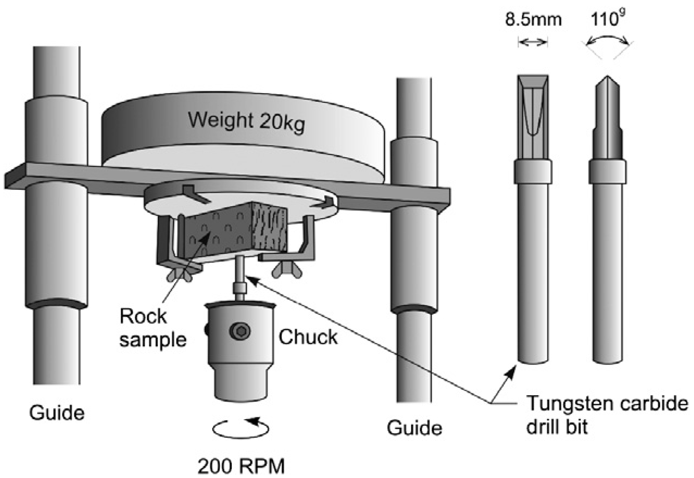
2.1.1. The Sievers’ Miniature Drill Test

In order to evaluate the surface hardness of the rock, the Sj test was developed by H. Sievers in the 1950s. The Sievers’ J-value is the depth of the drilled hole after 200 revolutions of the drill bit which is measured in 1/10 of mm. This test should be repeated 4 to 8 times and the mean value should be used as the final number [24]. The test showing a schematic view of the test is performed on a sawn sample (Figure 1).

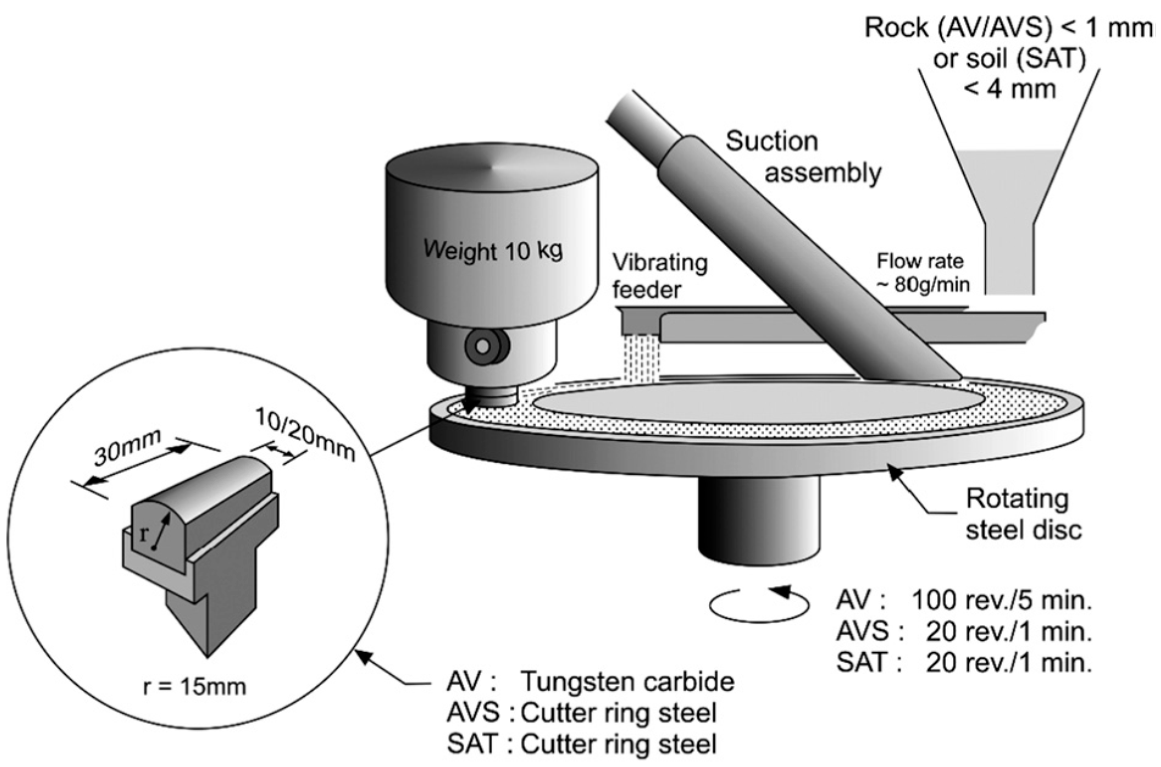
2.1.2. The Abrasion Value Steel

In abrasion value steel (AVS), rock powder in the size range of less than 1 mm is used to abrade the worn piece made of steel from a new cutter ring. The wear piece is under 10 kg dead load to increase the friction and contact pressure between rock grains and steel anvil. AVS is the weight loss of the worn piece after 20 rounds (1 min) of turn table rotation, which is measured in milligrams. Figure 2 shows the abrasion test and equipment [23,24].

2.1.3. Calculation of Cutter Life Index

After measurement of the AVS and SJ values, CLI can be calculated using the following formula. This formula is based on the real field data on actual cutter lifetime and related tested rock parameters.

$$\mathrm{CLI}=13.84·{\left[\frac{\mathrm{SJ}}{\mathrm{AVS}}\right]}^{0.3847}$$

(1)

From CLI,

$$\mathrm{CL}=\mathrm{CLI}·\mathrm{ROP}·\mathrm{A}$$

(2)

Cutter life (CL) can be computed as a function of CLI, rate of penetration (ROP), and cross section area of the opening (A) within m³/cutter. The cutter life index intervals are given in

Table 2. Category of intervals for cutter life index in NTNU Model [24].

Category	CLI
Extremely low	<5
Very low	5.0–5.9
Low	6.0–7.9
Medium	8.0–14.9
High	15.0–34
Very high	35–74
Extremely high	≥75

as suggested in the literature [24].

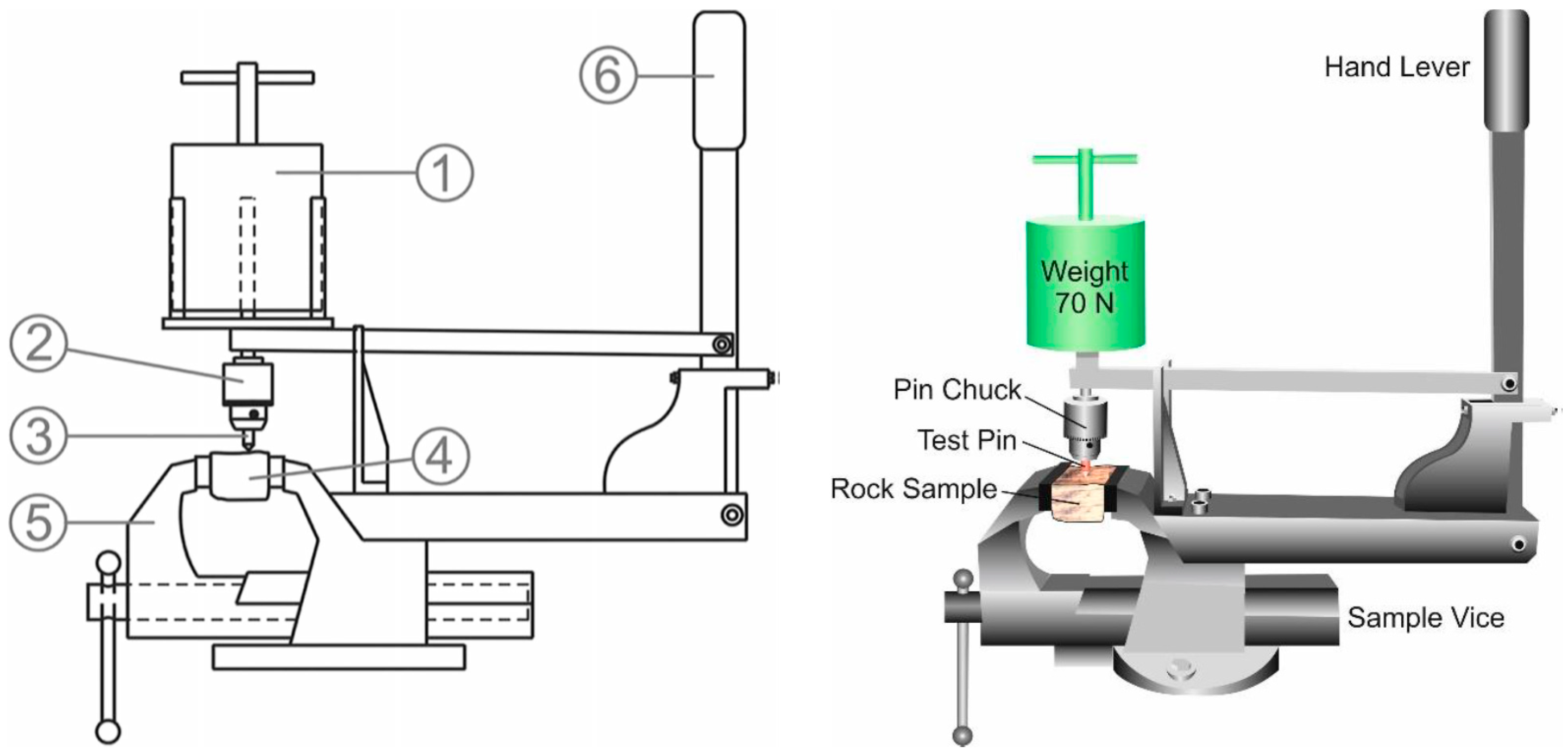
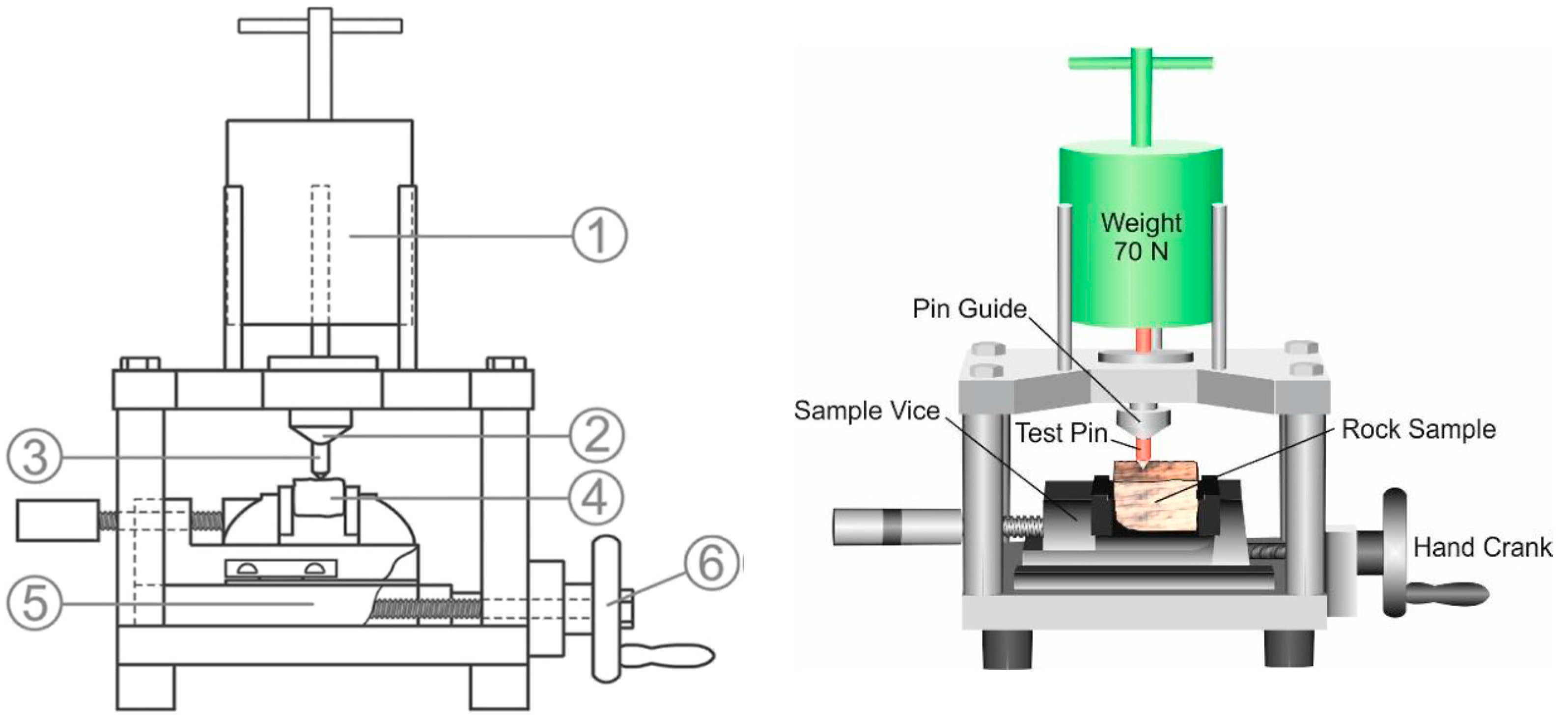
2.2. Cerchar Abrasivity Index (CAI)

Abrasivity is a good indicator of the wear life of cutting tools in any rock excavation operation. CAI is used for estimating the cutting tool life in the TBM performance prediction model of the Colorado School of Mines (CSM). Various rock abrasivity measurements have been introduced throughout the years to allow engineers to estimate cutting tool life. CAI is commonly utilized to characterize the abrasivity of rocks for estimation of cutting tool life and wear in various mining, civil and tunneling applications. The CAI [7] test has been introduced in the 1970s by the Centre d’Etudes et Recherches des Charbonages (CERCHAR) de France for abrasivity testing in coal-bearing rocks in mining industries while gradually being adopted for application in the tunneling industry [15,25,26,27]. Different generations of testing devices and the impact of various testing parameters on the test results have been discussed in the literature [15,18,28,29,30,31,32,33]. A typical CAI device is given in Figure 3 and Figure 4. A typical rock sample and surface used for CAI is given in Figure 5.

The CAI should be calculated as:

$$\mathrm{CAI}=\mathrm{d}·10$$

(3)

where d is the wear tip surface measured to an accuracy of 0.01 mm. The dimensionless CAI value is reported as the arithmetic mean of five or more test replications together with standard deviation as suggested by [9]. While the original formal standard of the test was the French standard NF P 940-430-1 [34], recently an ASTM [8] and ISRM [9] standards for Cerchar testing were published. An effect of some Cerchar test parameters, including Cerchar pin properties, loading condition, and test length on the rock surface, on the values of CAI are given in Table 3.

Table 3. Effect of some Cerchar test parameters on the measured values of CAI [35].

Testing Factors	Effect on CAI Value
Test length	About 70% of wear occurs in the initial first millimeter of the scratch length, approximately 85% of after 2 mm of test slide, and only 15% of the wear flat is produced by the remaining 8 mm length [1,29,36,37]. In cases of harder and more abrasive rocks the CAI value length [38,39].
Static load	The CAI value increases linearly by changing static loads on the stylus [40,41].
Testing speed	The testing speed does not affect the CAI values significantly and commonly higher when conducted with 43 HRC pins at slow testing speeds [2,41]. The standardized testing speed is 10 mm/s for articulated hand lever type machine and 1 mm/s for hand-crank types [7,9].
Stylus hardness	Higher CAI values are obtained with soft CERCHAR test styli and vice versa [36,38,41,42,43,44,45].
Stylus metallurgy	No considerable effect on CAI value is observed by changes in the metallurgy of the stylus keeping regular hardness [43].

Table 3. Effect of some Cerchar test parameters on the measured values of CAI [35].

Testing Factors	Effect on CAI Value
Test length	About 70% of wear occurs in the initial first millimeter of the scratch length, approximately 85% of after 2 mm of test slide, and only 15% of the wear flat is produced by the remaining 8 mm length [1,29,36,37]. In cases of harder and more abrasive rocks the CAI value length [38,39].
Static load	The CAI value increases linearly by changing static loads on the stylus [40,41].
Testing speed	The testing speed does not affect the CAI values significantly and commonly higher when conducted with 43 HRC pins at slow testing speeds [2,41]. The standardized testing speed is 10 mm/s for articulated hand lever type machine and 1 mm/s for hand-crank types [7,9].
Stylus hardness	Higher CAI values are obtained with soft CERCHAR test styli and vice versa [36,38,41,42,43,44,45].
Stylus metallurgy	No considerable effect on CAI value is observed by changes in the metallurgy of the stylus keeping regular hardness [43].

Rock abrasivity could be also examined based on the weighted average abrasivity of the constituent minerals. In this method, the percentage of each mineral in the rock is calculated and multiplied by its hardness or abrasivity, based on different available scales [21]. Abrasive mineral content (AMC), equivalent quartz content (EQC), and Vickers hardness number for rock (VHNR) are the most common methods to compute the abrasivity of rocks. AMC uses Mohs scratch hardness, while EQC uses Rosiwal [46] grinding hardness and VHNR benefits from Vickers indentation hardness (an indentation test in which the ratio of the force to the area of the indentation is considered as an index for abrasivity of the material) [21]. In the EQC method, constituent minerals of the rock would be identified either by microscopic or macroscopic mineral examination. Common methods utilized for abrasion measurement of rocks are given in Table 4.

Table 4. Common methods utilized for abrasion measurement and classification [47].

Method	Remarks	Advantage	Disadvantage	Ref.
Mohs scale	Mineral comparative scratch test	Simple to use	It is just a qualitative measure	[48]
Vickers hardness number rock (VHNR)	Based on indentation hardness (the ratio of force to the area of indentation) using a diamond tipped micro-indenter (Vickers)	Simple method to rate rock wear capacity based on available charted mineral VHNR values	Limited experience for TBM rock cutting	[40]
Rock abrasive index (RAI)	RAI = UCS × EQC	Simple method Presence of a chart for conical pick life	No chart for disc cutter life prediction	[30]
Abrasive mineral content	Uses Mohs scratch hardness	Simple to use	Limited experience for TBM rock cutting	[21]
Equivalent quartz content	Uses Rosiwal rating	Simple to use	Limited experience for TBM rock cutting	[21]
Wear index-F	F = Q × D.z.10 = equivalent quartz percentage, D—mean quartz grain size in mm, z—Brazilian tensile strength in MPa	Is developed for drag tool cutting	Specimen mean quartz grain size has high importance in the formula. In coarse grained metamorphic and igneous rocks, this index may lead to highly misleading results	[6]
Rosiwal mineral abrasivity rating	Rosiwal = 1000 × volume loss corundum/volume loss mineral specimen	Simple to use	Limited experience for TBM rock cutting	[46]
NTNU cutter life index (CLI)	CLI is obtained from AVS and Siever’s J tests	Large database and presence of disc cutter life prediction charts	Correct tests can only be performed in SINTEF and the replicated testing equipment may show results with high discrepancy	[49]
Cerchar abrasivity index (CAI)	Steel pin tip diameter in 1/10th mm after 1 cm scratch test under 70N normal load	Widely used test in tunneling, simple, low cost, low sample requirement	Good only for rough surfaces, variability in the test results due to its sensitivity to method of tip reading, the rock surface condition, the non-constant cross-section of pin tip during the test	[50]

Table 4. Common methods utilized for abrasion measurement and classification [47].

Method	Remarks	Advantage	Disadvantage	Ref.
Mohs scale	Mineral comparative scratch test	Simple to use	It is just a qualitative measure	[48]
Vickers hardness number rock (VHNR)	Based on indentation hardness (the ratio of force to the area of indentation) using a diamond tipped micro-indenter (Vickers)	Simple method to rate rock wear capacity based on available charted mineral VHNR values	Limited experience for TBM rock cutting	[40]
Rock abrasive index (RAI)	RAI = UCS × EQC	Simple method Presence of a chart for conical pick life	No chart for disc cutter life prediction	[30]
Abrasive mineral content	Uses Mohs scratch hardness	Simple to use	Limited experience for TBM rock cutting	[21]
Equivalent quartz content	Uses Rosiwal rating	Simple to use	Limited experience for TBM rock cutting	[21]
Wear index-F	F = Q × D.z.10 = equivalent quartz percentage, D—mean quartz grain size in mm, z—Brazilian tensile strength in MPa	Is developed for drag tool cutting	Specimen mean quartz grain size has high importance in the formula. In coarse grained metamorphic and igneous rocks, this index may lead to highly misleading results	[6]
Rosiwal mineral abrasivity rating	Rosiwal = 1000 × volume loss corundum/volume loss mineral specimen	Simple to use	Limited experience for TBM rock cutting	[46]
NTNU cutter life index (CLI)	CLI is obtained from AVS and Siever’s J tests	Large database and presence of disc cutter life prediction charts	Correct tests can only be performed in SINTEF and the replicated testing equipment may show results with high discrepancy	[49]
Cerchar abrasivity index (CAI)	Steel pin tip diameter in 1/10th mm after 1 cm scratch test under 70N normal load	Widely used test in tunneling, simple, low cost, low sample requirement	Good only for rough surfaces, variability in the test results due to its sensitivity to method of tip reading, the rock surface condition, the non-constant cross-section of pin tip during the test	[50]

2.3. Mechanical Properties of Rocks

Both intact rock and rock mass properties are used as the main parameters for estimating the project time and cost for a tunneling project. Tool consumption and machine advance rate in any rock mass are very closely related to the rock parameters such as strength, brittleness, density, abrasivity, mineral content. In this paper, several common rock properties were examined to estimate cutter consumption based on rock properties.

2.3.1. Rock Strength

The uniaxial compressive strength (UCS) and Brazilian tensile strength (BTS) are two of the most important and commonly measured rock properties for rock excavation projects since those strengths are related to both, porosity, density, and brittleness behavior of rock under the indenter/cutter. Due to the importance of the strengths, both the BTS and UCS values of the rocks are measured according to the standards [8,9] and recorded in the database.

2.3.2. Density and Porosity

Density (D) and porosity of rocks are both crucial parameters and hence are commonly utilized for estimating the cutter consumption and machine performance. The density and porosity of rocks could be measured using standard procedures (either [8] or [9]). In this study, density is used as one of the input parameters to estimate the CLI.

2.3.3. Rock Brittleness

The brittleness (BI_i) value is another fundamental rock property that should be considered for the assessment of boreability and cutter consumption; however, there are no universally accepted standards to measure brittleness. Yagiz (2009) discussed various approaches to represent rock brittleness directly from the punch penetration test (PPT). However, the PPT test is not a commonly used and available test. Several alternative rock brittleness based on rock strength ratios introduced in the literature [10,11,13] are as follow:

$${\mathrm{B}}_1=\frac{{\mathsf{\sigma }}_{\mathrm{c}}}{{\mathsf{\sigma }}_{\mathrm{t}}}$$

(4)

$${\mathrm{B}}_2=\frac{{\mathsf{\sigma }}_{\mathrm{c}}-{\mathsf{\sigma }}_{\mathrm{t}}}{{\mathsf{\sigma }}_{\mathrm{c}}+{\mathsf{\sigma }}_{\mathrm{t}}}$$

(5)

$${\mathrm{B}}_3=\sqrt{\frac{{\mathsf{\sigma }}_{\mathrm{c}}·{\mathsf{\sigma }}_{\mathrm{t}}}{2}}$$

(6)

where ${\mathsf{\sigma }}_{\mathrm{c}}$ is the compressive strength, ${\mathsf{\sigma }}_{\mathrm{t}}$ is the Brazilian tensile strength and ${\mathrm{B}}_1$, ${\mathrm{B}}_2$, ${\mathrm{B}}_3$ are brittleness indexes. As seen from the equations, all of them are different functions of the ratio of UCS to BTS. Although the BI is a function of the different combinations of rock properties rather than only ratios of the strength, there is no agreement on the measurement of the BI at the present time. Yagiz [13] has also introduced the BI value based on PPT and published equations that could be used for computing BI as follow:

$${\mathrm{BI}}_{\mathrm{o}}=\frac{F_{max}}{P_{max}}$$

(7)

where, F_max is the max force and P_max is the corresponding penetration

$${\mathrm{BI}}_{\mathrm{p}}=0.19\times {\mathsf{\sigma }}_{\mathrm{c}}-2.174\times { \mathsf{\sigma }}_{\mathrm{t}}+0.913\times \mathsf{\rho }-{3.807}_{ }$$

(8)

He stated that the brittleness of a rock cannot be only identified based on the strengths of a rock, but also related to density or porosity as well. It should be mentioned that the BI used herein is directly measured from the laboratory PPT and computed as suggested by past studies [13].

3. Database Development

In this paper, 80 tunnel cases are used to examine the effect of rock properties including UCS, BTS, density (D), brittleness (BI_i) that is measured from the punch penetration tests (PPT), Cerchar abrasivity index of rocks on the disc cutter consumption. Unpublished data obtained from various sources [51] were utilized for this purpose. Rock types range from sedimentary, igneous, and metamorphic, to volcanic rocks. Rock strength, (UCS and BTS), density, and CAI was conducted in accordance with ISRM standards; however, punch penetration tests were performed according to the Colorado School of Mines testing procedure [13]. The PPT test is conducted, examined and the brittleness value was calculated directly from the tests based on Yagiz’s Method [13,16]. To examine the effect of rock properties on the CLI, first CLI is computed as a function of CAI as follows [5]:

$$\mathrm{CLI}=2.87·{\mathrm{CAI}}^2-35.62·\mathrm{CAI}+112.9$$

(9)

In the dataset UCS of rock ranges from 9.5 to 317 MPa with averaged UCS values of rocks are 135 MPa. According to the ISRM classifications [52], the rock ranges from weak to very strong rock types. The BTS ranges from 2.5 to 17 with an average of 8.2 MPa. The density of rock ranges from 18 to 29.5 kN/m³; however, most of the rock samples had a density of around 25–28. The BI values range from 46 (very high brittle rock) to ductile rock according to the classification recently published [32]. The qualitative statistical evaluation of the data is summarized in

Table 5. Summary of rock properties and data ranges used for this paper [32].

Variables	N	Minimum	Maximum	Mean	Std. Dev.	Variance
D	80	17.69	29.53	25.70	2.03	4.14
UCS	80	9.50	327.00	131.24	54.91	3015.40
BTS	80	2.30	17.80	8.17	2.85	8.14
BI	80	9.68	46.00	27.78	8.55	73.09
CAI	80	0.66	6.40	3.52	1.27	1.62
CLI	80	2.49	90.64	27.68	22.32	498.02
Valid N	80

.

CAI is dependent on rock strength and other properties such as quartz content, and brittleness. The CAI values in the database varied from 6.4 (extremely abrasive) to 0.66 (low abrasivity) according to the ISRM classification [9]. Furthermore, the cutter consumption rate is represented by CLI and estimated by examining different approaches [5,14,15,37]. CLI was computed as suggested by past studies [5,26].

4. Development of CLI Models

The established dataset is used to experiment with a series of models with different input parameters to obtain the best reliable model to estimate the CLI on the basis of the rock properties. The SPSS Statistics [53] program was used as a statistical tool for this research together with other artificial intelligence techniques including artificial neural network (ANN) and fuzzy logic (FL) developed in the Matbal program [54]. A simple regression analysis was first performed between a single variable and CLI in order to evaluate the influence of each individual parameter on that. Multiple linear (MLRM) and non-linear models (NLMRM) were subsequently run in order to obtain the most accurate equations from the datasets. In order to examine empirical correlations between variables methods, statistical software packages such as Excel or SPSS are commonly utilized.

4.1. Regression Analysis of Data

4.1.1. Simple Regression Analysis (Univariate)

In this study, non-linear (y = ax^b) simple regression analyses were performed among rock properties to find the best inputs to estimate the CLI. This means that CLI was used as a dependent, while other rock properties were used as independent variables to develop pertinent models. This resulted in several simple regression relations among the possible input variables and CLI. Plots of CLI as a function of individual parameters are shown in Figure 6, Figure 7, Figure 8 and Figure 9.

4.1.2. Linear and Non-Linear Multi-Variable Regression Analysis

The prediction of CLI based on other rock properties can be carried out either using a linear or non-linear model. However, it is known that one of the common CLI estimation models from CAI [5] is polynomial a function. In this study, both linear and non-linear multivariable regression analyses were performed. While running the SPPS program, data were divided into two sets including: a training set (70%) and a testing set (30%).

Table 6. Summary of multi-variable statistical analysis of database using linear functions. statistical indices (#).

#	1	2	4	4	5	6	7
R	0.84	0.82	0.73	0.77	0.65	0.77	0.78
R2	0.71	0.67	0.53	0.60	0.42	0.59	0.62
MSE	135.97	148.57	212.52	171.47	289.83	201.65	159.59
RMSE	11.66	12.19	14.58	13.09	17.02	14.20	12.63

Inputs: ¹ UCS, BTS, D, BI; ² UCS, D, BTS; ³ UCS, BTS; ⁴ UCS, D; ⁵ UCS, BI; ⁶ BTS, BI; ⁷ D, BI.

is the summary of bi-linear multiple regression together with input variables of each model and statistical indices (#).

In this study, 7 different models were developed using both linear and non-linear regression as shown in Table 6. The results are very close to each other which means each rock property has some effect on CLI; hence, the models and related equations are listed in

Table 7. Results of multi-variable linear regression of CLI as function of other rock properties.

#	Inputs	Equations for CLI
1	D, UCS, BTS, BI	$\mathrm{CLI} =-4.425\times \mathrm{D}+0.079\times \mathrm{UCS}-3.408\times \mathrm{BTS}-0.735\mathrm{BI}+180.855$
2	D, UCS, BTS	$\mathrm{CLI} =-4.928\times \mathrm{D}-0.005\times \mathrm{UCS}-3.24\times \mathrm{BTS}+183.232$
3	UCS, BTS	$\mathrm{CLI} =-0.048\times \mathrm{UCS}-4.601\times \mathrm{BTS}+74.176$
4	D, UCS	$\mathrm{CLI} =-6.055\times \mathrm{D}-0.108\times \mathrm{UCS}+198.304$
5	UCS, BI	$\mathrm{CLI} =-0.106\times \mathrm{UCS}-1.01\times \mathrm{BI}+70.595$
6	BTS, BI	$\mathrm{CLI} =-3.991\times \mathrm{BTS}-0.761\times \mathrm{BI}+83.729$
7	D, BI	$\mathrm{CLI} =-5.858\times \mathrm{D}-0.824\times \mathrm{BI}+201.505$

. The best model obtained via MLRM is given in Figure 10 and Figure 11.

Similarly, multi-variable non-linear regression output equations and related performance indices are given in

Table 8. Summary of non-linear multi-variable statistical analysis of CLI.

Non-L	1	2	4	4	5	6	7
R	0.85	0.83	0.79	0.76	0.69	0.81	0.79
R2	0.72	0.69	0.62	0.58	0.47	0.66	0.62
MSE	124.88	138.22	154.67	167.51	235.07	159.15	154.71
RMSE	11.18	11.76	12.44	12.94	15.33	12.62	12.44
VAF	72.33	68.86	62.39	57.58	47.30	66.01	62.07

and

Table 9. Results of multi-variable non-linear regression of CLI as function of other rock properties.

	Inputs	Equations for CLI
1	D, UCS, BTS, BI	$$\begin{gathered} -4.099\times \mathrm{D}+9.771\times \mathrm{Ln}\left(\mathrm{UCS}\right)-30.94\times \mathrm{Ln}\left(\mathrm{BTS}\right)-0.006\times { \mathrm{BI}}^2 \\ -0.361\times \mathrm{BI}+166.102 \end{gathered}$$
2	D, UCS, BTS	$-3.938\times \mathrm{D}+2.251\times \ln \left(\mathrm{UCS}\right)-32.179\times \ln \left(\mathrm{BTS}\right)+185.433$
3	UCS, BTS	$-3.38\times \ln \left(\mathrm{UCS}\right)-40.63\times \ln \left(\mathrm{BTS}\right)+128.817$
4	D, UCS	$-5.741\times \mathrm{D}-10.418\times \ln \left(\mathrm{UCS}\right)+225.352$
5	UCS, BI	$-13.933\times \ln \left(\mathrm{UCS}\right)+0.025\times { \mathrm{BI}}^2-2.258\times \mathrm{BI}+136.543$
6	BTS, BI	$-35.366\times \ln \left(\mathrm{BTS}\right)+0.018\times { \mathrm{BI}}^2-1.604\times \mathrm{BI}+131.049$
7	D, BI	$-6.344\times \mathrm{D}-0.018\times { \mathrm{BI}}^2+0.256\times \mathrm{BI}+199.683$

, respectively, for each alternative model developed using the other rock properties. It could be stated that each rock property has some weight on CLI.

The results of the analysis for both linear and non-linear multi-variable regression show that models with three inputs can offer a reliable estimate of CLI with a coefficient of correlation of 0.82. This is very close to the correlation coefficient obtained from model 1 for training and testing data, respectively (Figure 12 and Figure 13).

It should be noted that the linear regression analysis approach has clear advantages over the black box models provided by AI systems, simply by offering equations for use by everyone.

4.2. Soft Computing Techniques

Artificial intelligence (AI) is a common modeling technique for developing models to estimate an unknown parameter from knowing variables in rock engineering and tunneling as well as other engineering practices. In this research, two common artificial intelligence methods including artificial neural network (ANN) and fuzzy logic (FL) were utilized to estimate the CLI as a function of common rock properties including strength, density, and brittleness. Several alternative models with alternative input variables were developed and the best one among those models is highlighted herein.

4.2.1. Artificial Neural Networks (ANN)

The MATLAB environment [53] has a built-in application, neural net fitting tool, which is a computational tool that was used for developing an ANN model in this study. To set up input data for ANN analysis, it is required to set a portion of data for testing, validation, and training. In our case of 70% of input data was used for training purposes, another 15% was used for validation, and 15% was for testing [55]. ANN uses the Levenberg–Marquardt optimization algorithm due to its advantages, such as high speed of training on feed-forward networks of moderate size [56]. Moreover, the MATLAB environment has an efficient built-in function of the Levenberg–Marquardt algorithm with very efficient performance [57].

In this study, the ANN models were developed by using one hidden layer. Baheer and Hecht-Neilsen [58,59] claimed that neural networks with one hidden layer, in general, are enough for addressing the majority of issues. ANN models developed in the neural net fitting tool use a two-layer-forward network with linear output neurons, where one layer is the hidden layer and one is the output layer. This type of network is capable of solving multi-dimensional mapping issues with sufficient accuracy if ANN has reliable data for training and enough number of neurons for the hidden layer. The next step for the ANN model development is to define the number of neurons, which was considered to be the most crucial question in the process of determining the ANN structure [60]. If the number of hidden neurons is lower than needed, it will undergo the “under-fitting” problem in both generalization and training. Nevertheless, an excess number of hidden neurons can result in the problem of overfitting, which means the neural network overestimates the target problem’s complexity [61]. This can cause a large variance in prediction results, and the generalization capacity drops considerably. Without performing a try-and-test during training and calculating the generalization error, determining the best number of hidden units is difficult. The number of hidden layers and hidden neurons, that is optimal to certain cases, is determined by the following factors: (a) network design complexity; (b) the number of input and output units; (c) the number of training samples; (d) the level of noise in the sample dataset; (e) the training algorithm [62]. In this regard, determining the correct number of hidden neurons to avoid overfitting or underfitting is crucial in the prediction process. The heuristic parameters suggested for this purpose are listed in Table 10.

Table 10. The heuristics proposed for optimal number of neurons.

Heuristic	References
$\le 2 * {\mathrm{N}}_{\mathrm{i}}+ 1$	[59]
$3{\mathrm{N}}_{\mathrm{i}}$	[63]
$({\mathrm{N}}_{\mathrm{i}} + {\mathrm{N}}_{\mathrm{o}})/2$	[64]
$\frac{2+{\mathrm{N}}_o * {\mathrm{N}}_{\mathrm{i}}+0.5{\mathrm{N}}_{\mathrm{o}} * \left({\mathrm{N}}_{\mathrm{o}}^2+{\mathrm{N}}_{\mathrm{i}}\right)-3}{{\mathrm{N}}_{\mathrm{i}}+{\mathrm{N}}_{\mathrm{o}}}$	[65]
$\frac{2{\mathrm{N}}_{\mathrm{i}}}{3}$	[66]
$\sqrt{{\mathrm{N}}_{\mathrm{i}} * {\mathrm{N}}_{\mathrm{o}}}$	[67]
$2{\mathrm{N}}_{\mathrm{i}}$	[68]

Table 10. The heuristics proposed for optimal number of neurons.

Heuristic	References
$\le 2 * {\mathrm{N}}_{\mathrm{i}}+ 1$	[59]
$3{\mathrm{N}}_{\mathrm{i}}$	[63]
$({\mathrm{N}}_{\mathrm{i}} + {\mathrm{N}}_{\mathrm{o}})/2$	[64]
$\frac{2+{\mathrm{N}}_o * {\mathrm{N}}_{\mathrm{i}}+0.5{\mathrm{N}}_{\mathrm{o}} * \left({\mathrm{N}}_{\mathrm{o}}^2+{\mathrm{N}}_{\mathrm{i}}\right)-3}{{\mathrm{N}}_{\mathrm{i}}+{\mathrm{N}}_{\mathrm{o}}}$	[65]
$\frac{2{\mathrm{N}}_{\mathrm{i}}}{3}$	[66]
$\sqrt{{\mathrm{N}}_{\mathrm{i}} * {\mathrm{N}}_{\mathrm{o}}}$	[67]
$2{\mathrm{N}}_{\mathrm{i}}$	[68]

In Table 10, N_i refers to the number of input neurons and N_o refers to the number of output neurons, respectively. According to Table 10, the number of hidden neurons must be 1, 2, 5, or 6 for two inputs, while for a set of four input parameters, the number of hidden neurons was suggested to be between 2 and 12. However, the work of Ke and Liu [61] suggested that for 80 input samples and one hidden layer, the optimal number of neurons is 12. The trial-and-error approach is currently used to calculate the number of hidden neurons. This begins with a small number of neurons and progressively increasing the number till optimal performance is achieved. The downside is that it takes time and there is no assurance that the hidden neuron would be fixed [62].

To determine the number of hidden neurons, suggested heuristics in Table 10 were employed. Then, from 1 to 14 hidden neurons were used to establish the models, which were run at least 25 times to obtain the best output. This was followed by evaluating the performance of developed ANN models on the basis of average performance obtained, in terms of the R-value and MSE. The optimal number of hidden neurons was chosen as indicated in

Table 11. Number of hidden neurons for 80 sample inputs.

Input Parameters	# of Hidden Neurons
Density, UCS, BTS, BI	10
Density, UCS, BTS	8
UCS, BTS	9
Density, UCS	6
UCS, BI	8
BTS, BI	10
Density, BI	7

. An illustration of the ANN structure corresponding to four inputs with one hidden layer and 10 neurons is given in Figure 14.

Developed ANN structures with a given number of inputs involve another component of the structure that is established and run to obtain average values of the model outputs. The results from each model are examined using several statistical indices such as coefficient of determination (r²), correlation (r), and variance account for (VAF); root means square error (RMSE) and mean square error (MSE). A summary of the results for performance of various models is given in

Table 12. Statistical indices of the ANN models for calculation of CLI from other rock properties.

ANN	1	2	3	4	5	6	7
R	0.75	0.83	0.76	0.80	0.73	0.73	0.84
R2	0.57	0.68	0.57	0.64	0.54	0.53	0.71
MSE	168.89	137.79	173.64	186.01	193.45	301.09	145.67
RMSE	13.00	11.74	13.18	13.64	13.91	17.35	12.07
VAF	56.78	68.12	57.31	64.12	53.75	51.36	69.99

. It appears that each input rock property has some influence on the CLI and the output of model 7 is better than others. The best ANN model to estimate CLI is a function of the density and brittleness of rocks. The best results from various ANN models are given in Table 12, as a function of density and brittleness (BI) as a combination of rock properties (Figure 15 and Figure 16).

4.2.2. Fuzzy Logic (FL)

In this research, another artificial intelligence model that was developed is based on Fuzzy Logic (FL). FL model requires special rules to control data behavior. To obtain these rules and membership functions, the Matlab built-in function “genfis2” was used. This function uses provided input and output data in separate matrices as input arguments. It also requires radii to be selected for input and output arguments, which specifies the center of cluster range of influence for each of the dimensions used in the data set. The data was then used to estimate the amount of membership functions and rules for the antecedents and consequents. The extracted rules were stored in a special FIS format variable, that later could be used to obtain predicted output for certain input variables. Similar to Section 4.2.1, different input rock characteristics were used as inputs for the fuzzy logic model and 70% of data was used for training, and the remaining 30% was used for testing to estimate the CLI. The FL model was also performed for seven different combinations of rock properties, and the output of the models is discussed in this paper. The generated FIS file contains membership functions that define to what degree a certain input belongs to a given set. The following figures are a representation of the fuzzy logic model created by the “genfis2” command, where input parameters are density and UCS with the output of CLI. These membership functions are based on gbellmf (generalized bell-shaped membership function), which is a function with a specific shape suitable for this analysis. This function was chosen automatically by the genfis2 command. The “anfis” function in MATLAB software uses the adaptive neuro-fuzzy inference system (ANFIS) to tune the FIS file obtained from “genfis2” and its use was recommended in the literature [69]. This approach is especially useful in engineering fields where traditional methods fail or are too difficult to use [70]. The ANFIS technique is effective for nonlinear system interpretation [71]. The “Anfis” command in the MATLAB environment provided some improvement in the modeling results as shown by higher correlation factors and MSE. The results of the FL analysis of CLI are presented in the next section of this paper. The final visualization of rules for the FIS file after the “anfis” tuning command is used can be seen in Figure 17 with two input cases for the dataset.

Given that the MATLAB [54] fuzzy logic designer tool is not capable of extracting rules that control the behavior of data, it had to be carried out with the built-in command “genfis2”. To do so, input and output data were defined from the dataset, and then by using “dividerand” that sets what fraction of data can be used in training, testing, and validation; it randomly selects which samples of the dataset go to which part. The “genfis2” function is used on that randomly chosen 70% of data to be trained, then the “evalfis” command is used to check the model by predicting results on training and testing samples. It is performed inside of the loop where the variable “i” defines the radius of the cluster from 0.1 to 1 with 0.05 steps. Cluster radii is a scalar value, which is multiplied by the width of the data space. The “mse” code determines the MSE of models, while “mseALLtraining” collects these MSE measurements for finding optimal. After developing the rules and model structure for 80 tunneling cases to estimate the CLI as a function of rock properties, models run until they produce reliable and accurate results. To achieve the desired performance, seven different alternative input combinations were used and the results of the models were examined to find the best model among them. The initial steps involve evaluating the influence of each rock variable using the FL surface map as shown in Figure 18, Figure 19, Figure 20 and Figure 21.

As mentioned earlier, the FL models were run for various inputs as given in

Table 13. Statistical indices of the FL models obtained for each model.

FL	1	2	4	4	5	6	7
R	0.82	0.79	0.70	0.77	0.68	0.75	0.79
R2	0.68	0.63	0.48	0.60	0.47	0.57	0.63
MSE	170.22	195.74	272.03	212.35	280.70	226.94	197.14
RMSE	13.05	13.99	16.49	14.57	16.75	15.06	14.04
VAF	67.71	62.87	48.39	59.72	46.75	56.95	62.60

and the best model was Model#1; model 7 was also very promising with two instead of four input parameters. Overall observation indicates that model 7 with input parameters including density and brittleness is also valid and offers acceptable results for practical applications.

It was also observed that the FL modeling technique is a powerful tool to estimate CLI from other rock parameters. The plots of predicted and measured CLI of model 1 for testing and training are shown in Figure 22 and Figure 23, respectively.

In summary, various combinations of input parameters were used to examine the ability to predict CLI from other rock parameters and those models do not always produce reliable results, and the accuracy of the models depends on rock properties and the range of data in the original dataset used for modeling purposes.

5. Discussions

In this paper, four different methods were used to predict CLI from rock mechanical properties including UCS, BTS, density, and brittleness. For this purpose, a database of measured CLI and other rock mechanical properties was established and used in the analysis leading to the development of predictive models. These models were subsequently compared to each other via statistical indices. The analysis showed that the models offered a reasonable estimate of CLI, which can be used for the estimation of disc cutter consumption in the NTNU model.

Table 14. Comparison of accuracy of the models based on obtained statistical performance indices.

Inputs	BI
	UCS	UCS
	BTS	BTS	UCS	D	UCS	BTS	D
	D	D	BTS	UCS	BI	BI	BI
Linear	1	2	4	4	5	6	7
R	0.84	0.82	0.73	0.77	0.65	0.77	0.78
R2	0.71	0.67	0.53	0.60	0.42	0.59	0.62
MSE	135.97	148.57	212.52	171.47	289.83	201.65	159.59
RMSE	11.66	12.19	14.58	13.09	17.02	14.20	12.63
VAF	70.53	67.48	53.26	59.74	42.03	58.56	61.62
Non-L	1	2	3	4	5	6	7
R	0.85	0.83	0.79	0.76	0.69	0.81	0.79
R2	0.72	0.69	0.62	0.58	0.47	0.66	0.62
MSE	124.88	138.22	154.67	167.51	235.07	159.15	154.71
RMSE	11.18	11.76	12.44	12.94	15.33	12.62	12.44
VAF	72.33	68.86	62.39	57.58	47.30	66.01	62.07
ANN	1	2	3	4	5	6	7
R	0.75	0.83	0.76	0.80	0.73	0.73	0.84
R2	0.57	0.68	0.57	0.64	0.54	0.53	0.71
MSE	168.89	137.79	173.64	186.01	193.45	301.09	145.67
RMSE	13.00	11.74	13.18	13.64	13.91	17.35	12.07
VAF	56.78	68.12	57.31	64.12	53.75	51.36	69.99
FL	1	2	4	4	5	6	7
R	0.82	0.79	0.70	0.77	0.68	0.75	0.79
R2	0.68	0.63	0.48	0.60	0.47	0.57	0.63
MSE	170.22	195.74	272.03	212.35	280.70	226.94	197.14
RMSE	13.05	13.99	16.49	14.57	16.75	15.06	14.04
VAF	67.71	62.87	48.39	59.72	46.75	56.95	62.60

presents the comparative statistical indices for the four methods used for developing the models.

Since the output of the models, CLI, is sensitive to each rock property, obtained models give very similar results and it is not easy to choose the best among them. However, some of the models offer superior predictions compared to others depending on the number of input variables. For example, the models having two inputs including D and BI can offer reasonable results with only two parameters, however, BI requires punch penetration testing that is not very common. Yet, most of the models produced acceptable estimates of CLI.

6. Conclusions

In this paper, cutter consumption for TBMs as represented by CLI was examined and estimated as a function of several common rock properties to be used in practice. Datasets from several projects including uniaxial compressive strength, Brazilian tensile strength, density, and rock brittleness indices were compiled in a database and analyzed by various modeling techniques with different sets of input parameters. Statistical analysis (SPSS 26.0) software and MATLAB were used for the development of models based on regression and artificial intelligence models, respectively. The proposed models could estimate CLI, however, some of the models offered superior predictions.

Following are the the summary of findings in this study:

-

Rock properties including strength, UCS, BTS, density, and brittleness indices have some influence on the CLI.

-

Density and brittleness of rock are very important variables for estimating CLI and offer a better prediction of CLI compared to other variables. Moreover, while these two variables could be used for estimating the CLI when other parameters are not available, it is not recommended since density and BI do not reflect the abrasivity of the rock.

-

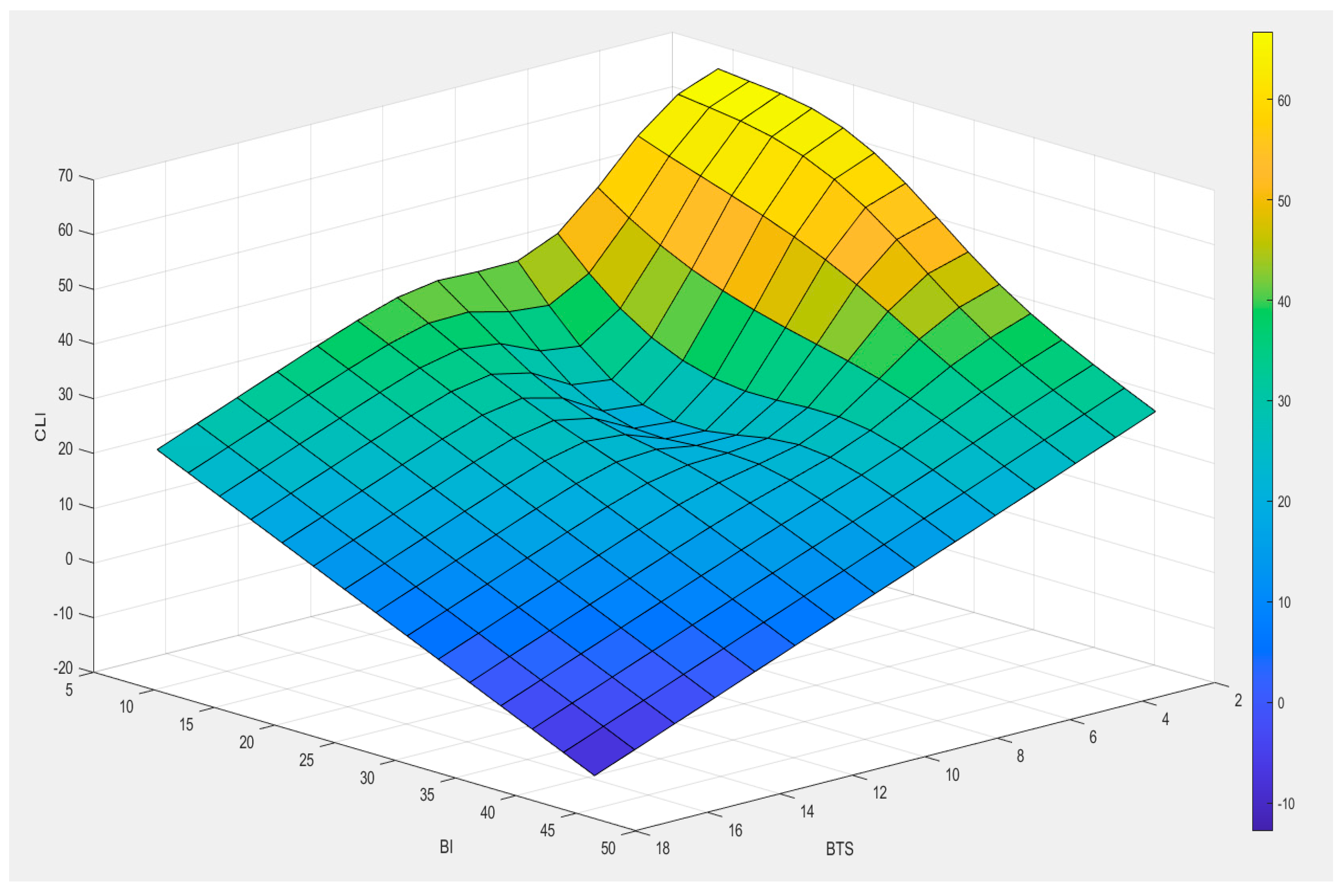
Brazilian tensile strength of rock is the significant input when it is used with BI (Model 6, non-linear model).

-

When comparing the variable for prediction of CLI on an individual basis, BTS shows a better correlation with CLI, perhaps since BTS is directly related to rock breakage and brittleness behavior of rock under the disc or indenter.

The dataset used in this study is based on real-world projects and proposed models could be valuable and applicable to practice; however, the output of the study should be improved by adding more rock data and inputs such as equivalent quartz content to the models.

References

1. Plinninger, R.J. Classification and Prediction of Tool Wear with Conventional, Mountain Solution Method in Solid Rock; Munich Geological Books, Series B, Applied Geology; IAEG: Munich, Germany, 2002. [Google Scholar]
2. Plinninger, R.J.; Kasling, H.; Thuro, K. Wear Prediction in Hardrock Excavation Using the CERCHAR Abrasiveness Index (CAI), EUROCK 2004 and 53rd Geomechanics Colloquium, ed.; Salzburg, Austria; pp. 599–604. Available online: http://www.plinninger.de/images/pdfs/2004_EUROCK_CAI.pdf (accessed on 1 December 2021).
3. Sun, Z.; Zhao, H.; Hong, K.; Chen, K.; Zhou, J.; Li, F.; Zhang, B.; Song, F.; Yang, Y.; He, R. A practical TBM cutter wear prediction model for disc cutter life and rock wear ability. Tunn. Undergr. Space Technol. 2019, 85, 92–99. [Google Scholar] [CrossRef]
4. Thuro, K.; Wilfing, L.; Wieser, C.; Ellecosta, P.; Käsling, H.; Schneider, E. Hard rock TBM Tunnelling—On the way to a better prognosis? Goeomechanics Tunn. 2015, 8, 191–199. [Google Scholar] [CrossRef]
5. Bruland, A. Hard Rock Tunnel Boring—Geology and Site Investigation. Project Report 1D-98; NTNU: Trondheim, Norway, 1998. [Google Scholar]
6. Schimazek, T.; Knatz, H. The influence of rock structures on the cutting speed and pick wear of heading machines. Glücckauf March 1970, 106, 275–278. (In German) [Google Scholar]
7. Cerchar. Centre d´ Etudes et Recherches de Charbonnages de France: The Cerchar Abrasiveness Index; Cerchar: Verneuil, France, 1986. [Google Scholar]
8. ASTM. Standard Test Method for Laboratory Determination of Abrasiveness of Rock Using the Cerchar Method; ASTM Designation 2010, D7625-10 Vol. 04.08; American Society for Testing and Materials: West Conshohocken, PA, USA.
9. Alber, M.; Yaralı, O.; Dahl, F.; Bruland, A.; Käsling, H.; Michalakopoulos, T.N.; Cardu, M.; Hagan, P.; Aydın, H.; Özarslan, A. ISRM Suggested Method for Determining the Abrasivity of Rock by the CERCHAR Abrasivity Test. Rock Mech. Rock Eng. 2014, 47, 261–266. [Google Scholar] [CrossRef]
10. Hucka, V.; Das, B. Brittleness determination of rocks by different methods. Int. J. Rock Mech. Min. Sci. Géoméch. Abstr. 1974, 11, 389–392. [Google Scholar] [CrossRef]
11. Altindag, R. Assessment of some brittleness indexes in rock-drilling efficiency. Rock Mech. Rock Eng. 2009, 43, 361–370. [Google Scholar] [CrossRef]
12. Andreev, G.E. Brittle Failure of Rock Materials: Test Results and Constitutive Models; A. A. Balkema: Rotterdam, The Netherlands, 1995; p. 446. [Google Scholar]
13. Yagiz, S. Assessment of brittleness using rock strength and density with punch penetration test. Tunn. Undergr. Space Technol. 2009, 24, 66–74. [Google Scholar] [CrossRef]
14. Rostami, J. Development of a Force Estimation Model for Rock Fragmentation with Disccutters through Theoretical Modeling and Physical Measurement of Crushed Zone Pressure. Ph.D. Thesis, Colorado School of Mines, Golden, CO, USA, 1997; p. 249. [Google Scholar]
15. Rostami, J.; Huckami, A.; Gharahbagh, E.A.; Dogruoz, C.; Dahl, F. Study of dominant factors affecting Cerchar abrasivity index. Rock Mech. Rock Eng. 2014, 47, 1905–1919. [Google Scholar] [CrossRef]
16. Yagiz, S. Development of Rock Fracture and Brittleness Indices to Quantify the Effects of Rock Mass Features and Toughness in the CSM Model Basic Penetration for Hard Rock Tunneling Machines. Ph.D. Thesis, Department of Mining Engineering, Colorado School of Mines, Golden, CO, USA, 2002; 289p. [Google Scholar]
17. Yagiz, S. Utilizing rock mass properties for predicting TBM performance in hard rock condition. Tunn. Undergr. Space Technol. 2008, 23, 326–339. [Google Scholar] [CrossRef]
18. Yagiz, S.; Rostami, J.; Ozdemir, L. Recommended rock testing methods for predicting TBM performance: Focus on the CSM and NTNU Models. In Proceedings of the ISRM International Symposium-5th Asian Rock Mechanics Symposium, Tehran, Iran, 24–26 November 2008; pp. 1523–1530. [Google Scholar]
19. Frenzel, C. Modeling Uncertainty in Cutter Wear Prediction for Tunnel Boring Machines. GeoCongress 2012, 2012, 3239–3247. [Google Scholar] [CrossRef]
20. Parsajoo, M.; Mohammed, A.S.; Yagiz, S.; Armaghani, D.J.; Khandelwal, M. An evolutionary adaptive neuro-fuzzy inference system for estimating field penetration index of tunnel boring machine in rock mass. J. Rock Mech. Geotech. Eng. 2021, 13, 1290–1299. [Google Scholar] [CrossRef]
21. Deketh, H. Wear of Rock Cutting Tools. In Wear of Rock Cutting Tools; CRC Press: Boca Raton, FL, USA, 2020. [Google Scholar]
22. Atkinson, T.; Cassapi, V.B.; Singh, R.N. Assessment of abrasive wear resistance potential in rock excavation machinery. Int. J. Min. Geol. Eng. 1986, 3, 151–163. [Google Scholar] [CrossRef]
23. Dahl, F. DRI, BWI, CLI Standards; NTNU: Trondheim, Norway, 2003. [Google Scholar]
24. Dahl, F.; Bruland, A.; Drevland Jakobsen, P.; Nilsen, B.; Grøv, E. Classifications of properties influencing the drillability of rocks, based on the NTNU/SINTEF test method. Tunnell. Undergr. Space Technol. 2012, 28, 150–158. [Google Scholar] [CrossRef]
25. Alber, M. Stress dependency of the Cerchar abrasivity index (CAI) and its effects on wear of selected rock cutting tools. Tunn. Undergr. Space Technol. 2008, 23, 351–359. [Google Scholar] [CrossRef]
26. Massalov, T.; Yagiz, S.; Rostami, J. Relationship between key rock properties and Cerchar abrasivity index for estimation of disc cutter wear life in rock tunneling applications. In Proceedings of the ISRM International Symposium, Eurock 2020—Hard Rock Engineering, Trondheim, Norway, 14–19 June 2020. 7p. [Google Scholar]
27. Yagiz, S.; Frough, O.; Rostami, J. Evaluation of rock brittleness indices to estimate Cerchar Abrasivity Index for disc cutter weariness. In Proceedings of the 54th US Rock Mechanics and Geomechanics Symposium, Golden, CO, USA, 28 June–1 July 2020. 5p. [Google Scholar]
28. West, G. Rock abrasiveness testing for tunnelling. Int. J. Rock Mech. Min. Sci. Géoméch. Abstr. 1989, 26, 151–160. [Google Scholar] [CrossRef]
29. Plinninger, R.J. Abrasiveness Assessment for Hard Rock Drilling. Géoméch. Tunn. 2008, 1, 38–46. [Google Scholar] [CrossRef]
30. Plinninger, R.J.; Spaun, G.; Thuro, K. Prediction and classification of tool wear in drill and blast tunnelling. Engineering Geology for Developing Countries. In Proceedings of the 9th Congress of the International Association for Engineering Geology and the Environment, Durban, South Africa, 16–20 September 2002. [Google Scholar]
31. Plinninger, R.; Käsling, H.; Thuro, K.; Spaun, G. Testing conditions and geomechanical properties influencing the CERCHAR abrasiveness index (CAI) value. Int. J. Rock Mech. Min. Sci. 2003, 40, 259–263. [Google Scholar] [CrossRef]
32. Yagiz, S.; Yazitova, A.; Karahan, H. Application of differential evolution algorithm and comparing its performance with literature to predict rock brittleness for excavatability. Int. J. Mining Reclam. Environ. 2020, 34, 672–685. [Google Scholar] [CrossRef]
33. Yaralı, O.; Yaşar, E.; Bacak, G.; Ranjith, P. A study of rock abrasivity and tool wear in Coal Measures Rocks. Int. J. Coal Geol. 2008, 74, 53–66. [Google Scholar] [CrossRef]
34. AFNOR. Roches Determination du Pouvoir Abrasive d’uneroche Partie 1: Essai de Rayure Avec Une Pointe. Project Report NF P 94-430-1, Paris. 2000. Available online: https://www.boutique.afnor.org/fr-fr/norme/nf-p944301/roches-determination-du-pouvoir-abrasif-dune-roche-partie-1-essai-de-rayure/fa107119/17746 (accessed on 1 December 2021).
35. Majeed, Y.; Abu Bakar, M.Z. Statistical evaluation of CERCHAR Abrasivity Index (CAI) measurement methods and dependence on petrographic and mechanical properties of selected rocks of Pakistan. Bull. Int. Assoc. Eng. Geol. 2016, 75, 1341–1360. [Google Scholar] [CrossRef]
36. Al-Ameen, S.I.; Waller, M.D. The influence of rock strength and abrasive mineral content on the Cerchar Abrasive Index. Eng. Geol. 1994, 36, 293–301, ISSN 0013-7952.. [Google Scholar] [CrossRef]
37. Jamal, R.; Özdemir, L.; Amund, B.; Filip, D. Review of issues related to Cerchar abrasivity testing and their implications on geotechnical investigations and cutter cost estimates. In Proceedings of the Rapid Excavation and Tunnelling Conference, Society for Mining, Metallurgy, and Exploration Incorporated, Seattle, WA, USA, 13–15 June 2005; pp. 15–29. [Google Scholar]
38. Fowell, R.; Bakar, A.; Zubair, M. A Review of the Cerchar and LCPC Rock Abrasivity Measurement Methods. In Proceedings of the 11th Congress of the International Society for Rock Mechanics, Lisbon, Portugal, 9–13 July 2007. [Google Scholar]
39. Hamzaban, M.-T.; Memarian, H.; Rostami, J. Continuous Monitoring of Pin Tip Wear and Penetration into Rock Surface Using a New Cerchar Abrasivity Testing Device. Rock Mech. Rock Eng. 2013, 47, 689–701. [Google Scholar] [CrossRef]
40. Ghasemi, A. Study of Cerchar Abrasivity Index and Potential Modifications for More Consistent Measurement of Rock Abrasion; The Pennsylvania State University, Department of Energy and Mineral Engineering: State College, PA, USA, 2010; 88p. [Google Scholar]
41. Hamzaban, M.; Memarian, H.; Rostami, J.; Ghasemi-Monfared, H. Study of rock-pin interaction in Cerchar abrasivity test. Int. J. Rock Mech. Min. Sci. 2007, 72, 100–108. [Google Scholar] [CrossRef]
42. Michalakopoulos, T.; Anagnostou, V.; Bassanou, M.; Panagiotou, G. The influence of steel styli hardness on the Cerchar abrasiveness index value. Int. J. Rock Mech. Min. Sci. 2006, 43, 321–327. [Google Scholar] [CrossRef]
43. Stanford, J.; Hagan, P. An Assessment of the Impact of Stylus Metallurgy on Cerchar Abrasiveness Index. In Proceedings of the Coal Operators’ Conference. Australia; 2009. Available online: https://ro.uow.edu.au/coal2009/ (accessed on 1 December 2021).
44. Kasling, H.; Thuro, K. Determining abrasivity of rock and soil in the laboratory. In Proceedings of the 11th IAEG Congress, Auckland, New Zealand, 5–10 September 2010; p. 235. [Google Scholar]
45. Gharahbagh, E.A.; Rostami, J.; Ghasemi, A.R.; Tonon, F. Review of rock abrasion testing. In Proceedings of the 45th US Rock Mechanics/Geomechanics Symposium, San Francisco, CA, USA, 26–29 October 2011; pp. 11–141. [Google Scholar]
46. Rosiwal, A. Neuere Ergebnisse der Härtebestimmung von Mineralien und Gesteinen.—Ein Absolutes Maß für die Härte spröder Körper.—Verhandlungen der k. k. Geologischen Reichsanstalt, 5+6: Pp. 117–147. (Recent Results of Hardness Determination of Minerals and Rocks. An Absolute Measure of the Hardness of Brittle Solids). Available online: https://www.zobodat.at/publikation_series.php?id=19695 (accessed on 1 December 2021).
47. Farrokh, E.; Kim, D.Y. A discussion on hard rock TBM cutter wear and cutterhead intervention interval length evaluation. Tunn. Undergr. Space Technol. 2018, 81, 336–357. [Google Scholar] [CrossRef]
48. Paez, C.V.G. Performance, Wear and Abrasion in Excavation Mechanized Tunneling in Heterogeneous Land. Ph.D. Thesis, Universitat Politècnica de Barcelona, Catalunya, Spain, 2014. [Google Scholar]
49. Johannessen, O. NTH Hard Rock Tunnel Boring. Project Report 1–94; NTH/NTNU: Trondheim, Norway, 1994. [Google Scholar]
50. West, G. A relation between abrasiveness and quartz content for some Coal Measures sediments. Int. J. Min. Geol. Eng. 1986, 4, 73–78. [Google Scholar] [CrossRef]
51. Yagiz, S. Unpublished Database Obtained from Different Mechanical Tunnel Cases; Earth Mechanics Institute of Colorado School of Mines: Golden, CO, USA, 2021. [Google Scholar]
52. Ulusay, R.; Hudson, J.A. (Eds.) ISRM Suggested Methods Published between 1974 and 2006 Are Compiled in The ISRM Blue Book: The Complete ISRM Suggested Methods for Rock Characterization, Testing and Monitoring: 2007–2014 Ankara, Turkey. Available online: https://link.springer.com/article/10.1007/s10064-009-0213-2 (accessed on 1 December 2021).
53. Statistical Software Package; SPSS 26.0; IBM: Armonk, NY, USA, 2020.
54. MATLab. 2021. Available online: https://www.mathworks.com/products/new_products/latest_features.html (accessed on 1 May 2021).
55. Yun, X.; Goodacre, R. On Splitting Training and Validation Set: A Comparative Study of Cross-Validation, Boot-strap and Systematic Sampling for Estimating the Generalization Performance of Supervised Learning. J. Anal. Test. 2018, 2–3, 249–262. [Google Scholar]
56. Mammadli, S. Financial time series prediction using artificial neural network based on Levenberg-Marquardt algorithm. Procedia Comput. Sci. 2017, 120, 602–607. [Google Scholar] [CrossRef]
57. Demuth, H.B.; Raele, M.H. Neural Network Toolbox User’s Guide for Use with Matlab; MathWorks: Natick, MA, USA, 2009. [Google Scholar]
58. Baheer, I. Selection of methodology for modeling hysteresis behavior of soils using neural networks. Comput. Aided Civ. Infrastruct. Eng. 2000, 5, 445–463. [Google Scholar] [CrossRef]
59. Hecht-Nielsen, R. Kolmogorov’s mapping neural network existence theorem. In Proceedings of the First IEEE International Conference on Neural Networks, San Diego, CA, USA, 16–18 October 1989; pp. 11–14. [Google Scholar]
60. Sonmez, H.; Gokceoglu, C.; Nefeslioglu, H.; Kayabasi, A. Estimation of rock modulus: For intact rocks with an artificial neural network and for rock masses with a new empirical equation. Int. J. Rock Mech. Min. Sci. 2006, 43, 224–235. [Google Scholar] [CrossRef]
61. Ke, J.; Liu, X. Empirical Analysis of Optimal Hidden Neurons in Neural Network Modeling for Stock Prediction. In Proceedings of the 2008 IEEE Pacific-Asia Workshop on Computational Intelligence and Industrial Application, Wuhan, China, 19–20 December 2008; Volume 2, pp. 828–832. [Google Scholar]
62. Sheela, K.G.; Deepa, S.N. Review on Methods to Fix Number of Hidden Neurons in Neural Networks. Math. Probl. Eng. 2013, 2013, 425740. [Google Scholar] [CrossRef] [Green Version]
63. Hush, D.R. Classification with neural networks: A performance analysis. In Proceedings of the IEEE International Conference on Systems Engineering, Dayton, OH, USA, 1–3 August 1989; pp. 277–280. [Google Scholar]
64. Ripley, B.D. Statistical aspects of neural networks. In Networks and Chaos-Statistical and Probabilistic Aspects; Barndoff Neilsen, O.E., Jensen, J.L., Kendall, W.S., Eds.; Chapman & Hall: London, UK, 1993; pp. 40–123. [Google Scholar]
65. Paola, J.D. Neural Network Classification of Multispectral Imagery. Master’s Thesis, The University of Arizona, Tucson, AZ, USA, 1994. [Google Scholar]
66. Wang, C. A Theory of Generalization in Learning Machines with Neural Application. Ph.D. Thesis, The University of Pennsylvania, Philadelphia, PA, USA, 1994. [Google Scholar]
67. Masters, T. Practical Neural Network Recipes in C++; Academic Press: Boston, MA, USA, 1994. [Google Scholar]
68. Kaastra, I.; Boyd, M. Designing a neural network for forecasting financial and economic time series. Neurocomputing 1996, 10, 215–236. [Google Scholar] [CrossRef]
69. Naderloo, L.; Alimardani, R.; Omid, M.; Sarmadian, F.; Javadikia, P.; Torabi, M.Y.; Alimardani, F. Application of ANFIS to predict crop yield based on different energy inputs. Measurement 2012, 45, 1406–1413. [Google Scholar] [CrossRef]
70. Cheng, C.B.; Cheng, C.J.; Lee, E.S. Neuro-fuzzy and genetic algorithm in multiple response optimization. Comput. Math. Appl. 2002, 44, 1503–1514. [Google Scholar] [CrossRef] [Green Version]
71. Arkhipov, M.; Krueger, E.; Kurtener, D. Evaluation of Ecological Conditions Using Bioindicators: Application of Fuzzy Modeling, Computational Science and Its Applications–ICCSA 2008; Springer: Belrin, Germany, 2008; pp. 491–500. [Google Scholar]
Figure 1. The Sievers’ miniature drill test [24].
Applsci 12 01446 g001
Figure 2. Outline of abrasion value (AV) and abrasion value cutter steel (AVS) [24].
Applsci 12 01446 g002
Figure 3. Setup of a first-generation Cerchar testing device [7]. (1) Weight, (2) pin chuck, (3) steel pin, (4) specimen, (5) vice, and (6) hand lever [1].
Applsci 12 01446 g003
Figure 4. Setup of a second-generation Cerchar testing device [28].
Applsci 12 01446 g004
Figure 5. Example of rock surface conditions with rough surface (left over from BTS test) used for CAI test.
Applsci 12 01446 g005
Figure 6. Relations between the density and CLI.
Applsci 12 01446 g006
Figure 7. Relations between the UCS and CLI.
Applsci 12 01446 g007
Figure 8. Relations between the BTS and CLI.
Applsci 12 01446 g008
Figure 9. Relations between the BI and CLI.
Applsci 12 01446 g009
Figure 10. Relations between the measured CLI and predicted CLI for training (model 1-MLRM).
Applsci 12 01446 g010
Figure 11. Relations between the measured CLI and predicted CLI for testing (model 1-MLRM).
Applsci 12 01446 g011
Figure 12. Relations between the measured CLI and predicted CLI for training (model 1-NLMRM).
Applsci 12 01446 g012
Figure 13. Relations between the measured CLI and predicted CLI for testing (model 1-NLMRM).
Applsci 12 01446 g013
Figure 14. Generalized structure of ANN used in this study.
Applsci 12 01446 g014
Figure 15. Relations between the actual and estimated CLI by ANN model 7 for training.
Applsci 12 01446 g015
Figure 16. Relations between the actual and estimated CLI by ANN model 7 for testing.
Applsci 12 01446 g016
Figure 17. Fuzzy logic rules for 2 inputs and 1 output.
Applsci 12 01446 g017
Figure 18. Fuzzy logic surface view for inputs (UCS and BTS) and CLI.
Applsci 12 01446 g018
Figure 19. Fuzzy logic surface view for inputs (D, UCS) and CLI.
Applsci 12 01446 g019
Figure 20. Fuzzy logic surface view for inputs (BI, UCS) and CLI.
Applsci 12 01446 g020
Figure 21. Fuzzy logic surface view for inputs (BTS, BI) and CLI.
Applsci 12 01446 g021
Figure 22. Relations between the actual CLI and estimated CLI by FL model 1 for training.
Applsci 12 01446 g022
Figure 23. Relations between the actual CLI and estimated CLI by FL model 1 for testing.
Applsci 12 01446 g023