1. Introduction
Flow is one of the most important variables in industrial environments, and its precise measurement is the foundation of process automation. It is an established method in the production, infrastructure and process industry [
1]. Electromagnetic flow metering (EMFM) is widely used for flow monitoring in research and industry [
1]. However, it requires a minimum conductivity of 5 µS/cm of the fluid of interest. For nonconductive and multiphase media, which include non-ionized gases, ceramics, fuels or oils, there is no equivalent volumetric flow-metering technique [
2].
NMR-based flow metering has proven to be a viable tool for multiphase flow detection in clinical applications and does not require a minimum conductivity [
3,
4]. Conventional high-field NMR measuring devices established on the market are rarely used in industry [
5]. The difficult system integration and the associated costs limit its applicability [
6]. In the high field NMR regime, strong alternating magnetic fields are a compromise between signal strength and field generation effort. For noninvasive flow metering through metal pipes, the reduced penetration depth of the radiofrequency (RF) signals is an additional obstacle [
7].
For field strengths similar to the Earth’s magnetic field or lower (<50 µT), these disadvantages are significantly attenuated. Low magnetic fields are easy to generate, can be varied rapidly, and the low frequency RF-signals penetrate deeper through metallic enclosures such as pipes [
7]. Initial research on low-field NMR techniques applied to flow metering is available [
8,
9]. This research has already demonstrated the feasibility of NMR-based flow measurement in the Earth’s magnetic field using induction coils [
10,
11]. However, for a precise flow-metering method at field strengths below 50 µT, magnetometers are the better choice. In this field regime, signal frequencies are expected to be in the lower kHz to Hz range. For these frequencies, magnetometers show a higher signal-to-noise ratio compared to induction coils [
7,
12].
While the most sensitive magnetometers were cryogenically cooled SQUID detectors for a long time, the first optically pumped magnetometers (OPM) are now commercially available. They allow measurements with comparable sensitivity at room temperature [
13]. The working principle of an OPM is based on alkali atoms in a vapor cell, which are spin-polarized by a laser. The spin polarization of the atoms couples to the magnetic field to be measured and generates a measurable frequency [
14].
Utilizing the high magnetic sensitivity of OPM also renders magnetic tracer particles obsolete. Magnetic tracer particles are ferromagnetic clusters of atoms or molecules. When mixed in a liquid, these particles differ from the solution in their magnetic properties. Thus, the determination of the fluid movement is facilitated by monitoring the positions of the magnetic particles [
15].
The present research demonstrates a noninvasive tracer-free flow metering procedure, which uses an OPM operating in the zero-to-ultra-low-field (ZULF) regime as the signal detector. In a first step, the medium to be analyzed (here: water) is pre-polarized. Then, a resonant RF-pulse applies a magnetic time stamp to the medium by changing the water polarization locally. This time stamp can be detected with magnetometers such as OPM downstream. The time difference between pulsing and detecting indicates the flow velocity of the medium. In essence, the apparatus performs a time-of-flight measurement, which also makes the procedure calibration-free.
2. Materials and Methods
2.1. Experimental Setup
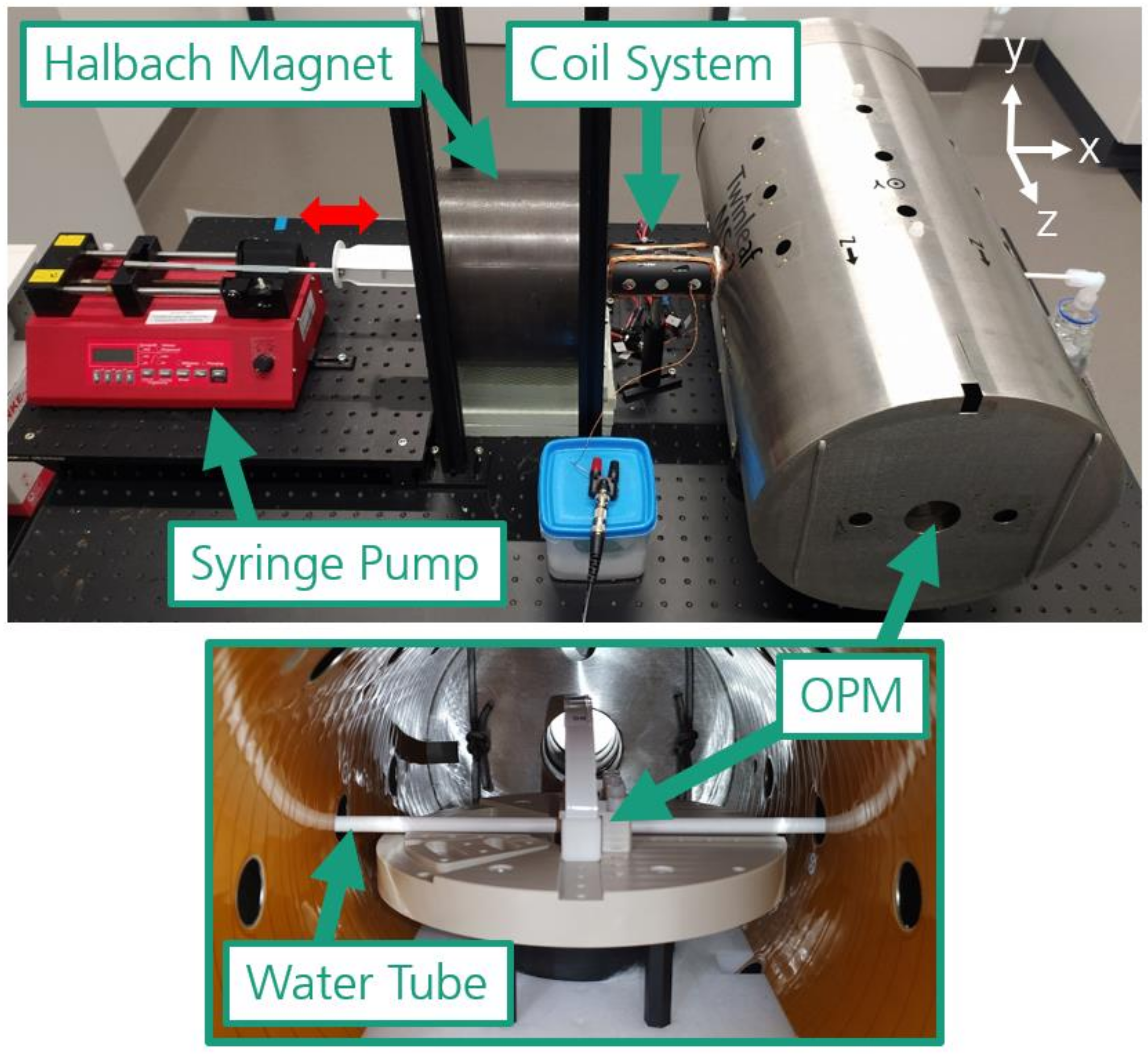
The experimental setup of the flow-metering apparatus and the orientation of the magnetic fields involved in the procedure is shown in
Figure 1 and
Figure 2. The water reservoir consisted of a plastic syringe of 200 mL capacity. The syringe was operated by a syringe pump (Syringe Pump LA-800, Landgraf, Langenhagen, Germany), which can log pump rates digitally. For pre-polarization of the water sample the syringe was placed inside a 1 T permanent magnet (RHR-1T-50 Halbach magnet, BFLUX TECHNOLOGY, Dublin, Ireland). This way the whole volume of the syringe could be polarized before being pushed into the system. Pre-polarization was used to increase the magnetic signal for the OPM detector to a measurable level [
7]. An interaction section and magnetic shielding (MS-2 Magnetic shield, Twinleaf LLC, Plainsboro Township, NJ, USA) containing magnetometers (Zero Field OPM, FieldLine Inc., Boulder, CO, USA.) were located downstream. The circuit ended in a water storage tank.
The interaction section consisted of a Helmholtz-coil (Ferronato®-BHC-2, Serviciencia, S.L.U., Toledo, Spain), which was used as an RF coil, and racetrack coils. The racetrack coils served a dual function of spin guiding between Halbach and shield, and providing a constant ambient magnetic field necessary for RF pulsing. The presence of a magnetic field is necessary for RF pulsing because a manipulation of the water polarization is not possible otherwise. In the presence of a magnetic field, the nuclear spin energy level of the hydrogen atom is split in two equidistant energy levels. This is called the Zeeman effect. To induce a transition between the energy levels, which define the macroscopic polarization of the water, an RF pulse with the transition frequency of the hydrogen can be applied. This transition frequency is called Larmor precession and is defined as . Here, is the gyromagnetic ratio of the proton, which is roughly 42.577 MHz/T, and is the strength of the ambient magnetic field. In the case of this experiment, the field generated by the racetrack coils was about 200 µT, which translates to an RF frequency of roughly 8 kHz.
The magnetic shield downstream contained zero field OPM for the detection of polarization changes induced by the RF coil. OPM are very sensitive sensors that can reach a sensitivity of 10
[
13] if they are operated in an environment where magnetic noise and the absolute magnetic field are strongly suppressed.
The distance between the center of the interaction section and the OPM was fixed at 212(1) mm throughout the experiment. A plastic tube with an inner diameter of 5 mm was used as a water guide. For validation, the data taken were compared to the pump rates indicated by the syringe pump in the end. Therefore, the flow velocity detected by the apparatus was converted to volumetric flow.
2.2. Procedure
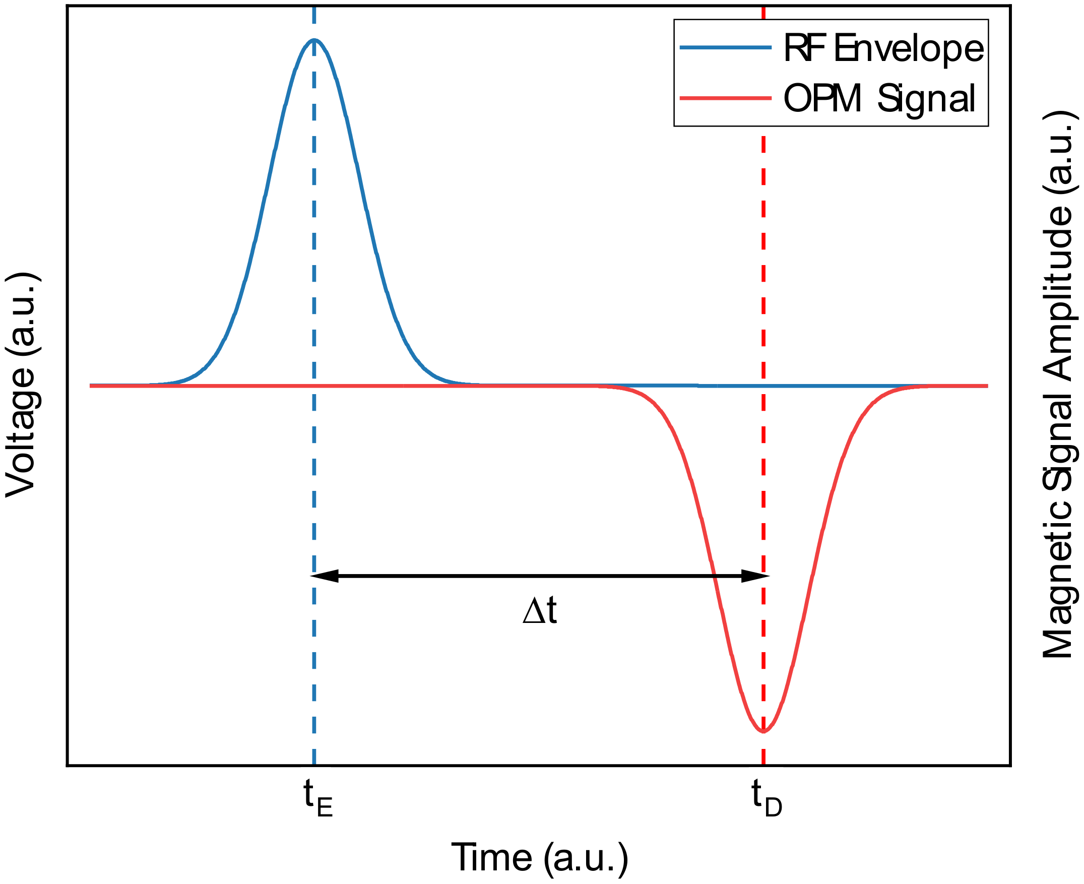
After starting the pump, the pre-polarized water flows through the apparatus. The water polarization interacts with the RF pulses of the RF coil in the interaction section (cf.
Figure 3). This coil is operated with amplitude modulation (AM). The 8 kHz RF signal has a sinusoidal envelope of 1 V at 100 mHz. The RF pulses manipulate the water polarization with an intensity proportional to the magnetic field generated by the AM RF coil. Thus, the RF coil periodically changes the polarization amplitude of the water passing the interaction section. Finally, the OPM detects an alternating magnetic amplitude of the water polarization analogue to the RF envelope. The time difference
between pulse application and detecting its effect on the water polarization yields the time information to calculate the flow velocity
v using the distance
:
To compare the measured flow rate to the pump rates indicated by the pump,
was converted to the average volumetric flow
Q inside the tube using the tube cross-section
A and its diameter
d.
2.3. Determination of ∆t
The voltage
U(
t) applied to the RF coil is a sinusoid
where
is the Larmor frequency and
is the modulated amplitude with a sinusoidal shape. To feed the RF coil, only the positive halfwave was used. Let the time of excitation
be defined as
. Then the detection time
is the corresponding point in time where the magnetic signal detected by the OPM is at its local minimum. An illustration of how the envelope RF voltage affects the magnetic signal recorded by the OPM is shown in
Figure 3. To determine
and
from the RF voltage and magnetic field data, parabolas were fitted to the raw data:
The horizontal shift of the function
and
were used to calculate ∆
t and determined as fit parameters. Thus,
is the time difference between
and
:
This method of data acquisition implies that we measure the average flow of water inside the tube. For demonstration purposes the AM frequency was set to 100 mHz.
3. Results
3.1. Volumetric Flow Measurement
Pump rates were varied from 150 mL/min to 275 mL/min in steps of 25 mL/min. According to Equation (2) these pump rates correspond to flow velocities from 12.7 cm/s to 23.3 cm/s. For this velocity range the maximum Reynolds Number
is
where
is the tube diameter,
is the density of water at 20 °C and
is the dynamic viscosity of water at 20 °C. Thus,
being smaller than
, we assume that we have laminar flow. Hence, the apparatus measures the laminar flow of water inside the tube.
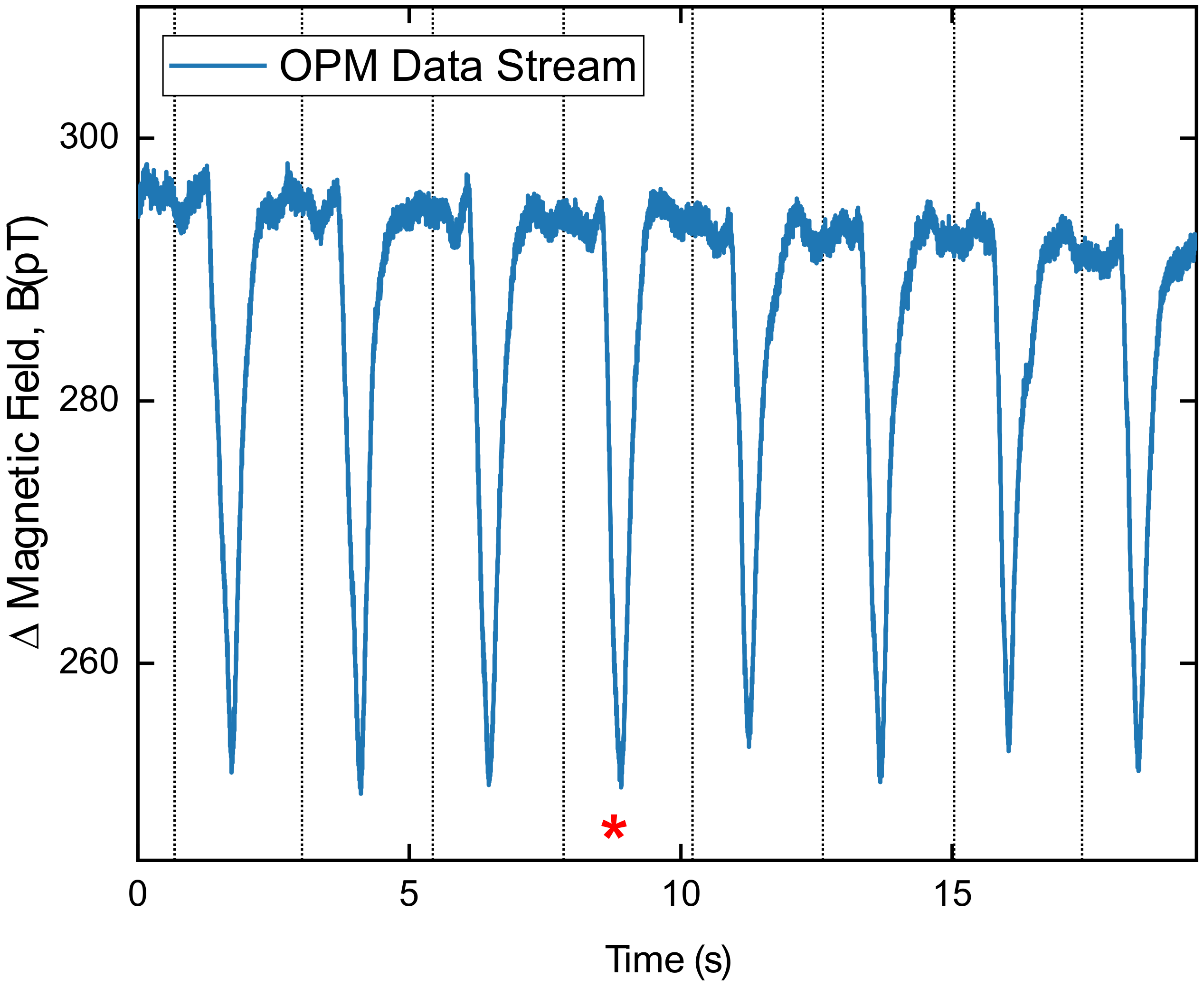
For each pump rate the syringe was emptied completely. The batch volume and the set pump rate determine the measuring time. In
Figure 4 streamed data from the 200 mL/min measurement are shown as an example. The OPM data were periodically modulated by the RF pulses and yielded a signal amplitude of about 60 pT. Please note that the Signal amplitude off-set was corrected in such a way that it was set to 0 before the start of the measurement.
The flow rate and volumetric flow calculation was done as explained in Equations (1) and (2). For each pump rate, data were recorded until the syringe was completely emptied. Depending on the flow rate, every measurement yielded 5 to 14 data points. The flow velocity for a given pump rate was determined by the average of the individual values
in one recording. The error on the average flow velocity was calculated from the scatter of the individual measured values for each pump rate. The results are listed in
Table 1 and shown in
Figure 5. On average, the relative error on the volumetric flow
and thus on the detected flow velocity
was 3%. In addition, the predicted pump rate of the syringe pump was mostly within one standard deviation of the detected volumetric flow. For 275 mL/min the predicted pump rate lays within two standard deviations.
For any practical application of the presented scheme, the dynamic range of the procedure was limited by two factors. The first limitation derived from the decay of the medium polarization. For too-small flow velocities, the signal would decay before it arrived in front of the sensor. The second limitation was caused by bandwidth of the OPM sensor (currently 100 Hz). This limited the accuracy of the determination of and, hence, of and the flow velocity.
3.2. Short RF Pulsing
In the experiments described above, the sinusoidal AM modulation of the RF pulses with 0.1 Hz limited both the data rate (one data point every 10 s) and the accuracy of the determination of . Shorter RF pulses are expected to produce narrower transients in the polarization signal, allowing one to determine more accurately and to increase the pulse rate.
In the following, an experiment was conducted as described in
Section 2.2 but rectangular RF pulses with a duration of 250 ms and a repetition rate of 0.4 Hz were applied. The flow velocity was set to of 12.7 cm/s. For comparison, the amplitude modulated RF pulse approach has a pulse length of 5 s. The RF amplitude in the experiment was 236 mV.
The experimental results are shown in
Figure 6. The mean full width at half-maximum (FWHM) of the observed transients of the magnetic field was 0.38(4) s. The specified error was calculated as the standard deviation (1 sigma) of the scattering data.
This width of the observed B field “pulses” was about 50% larger than the duration of the applied RF pulses (0.25 s). To get a first insight into the action of the RF pulses on the flowing water, a simple model was used: The change of macroscopic polarization for a pre-polarized water voxel was assumed to be proportional to the integral
experienced by the water voxel. Let
be the velocity of the water inside the tube. Then the magnetic field experienced by a water voxel
S starting to move at a point
inside the interaction section is given by
where
is the position of the water voxel and
is the magnetic field at this position. In a first approximation,
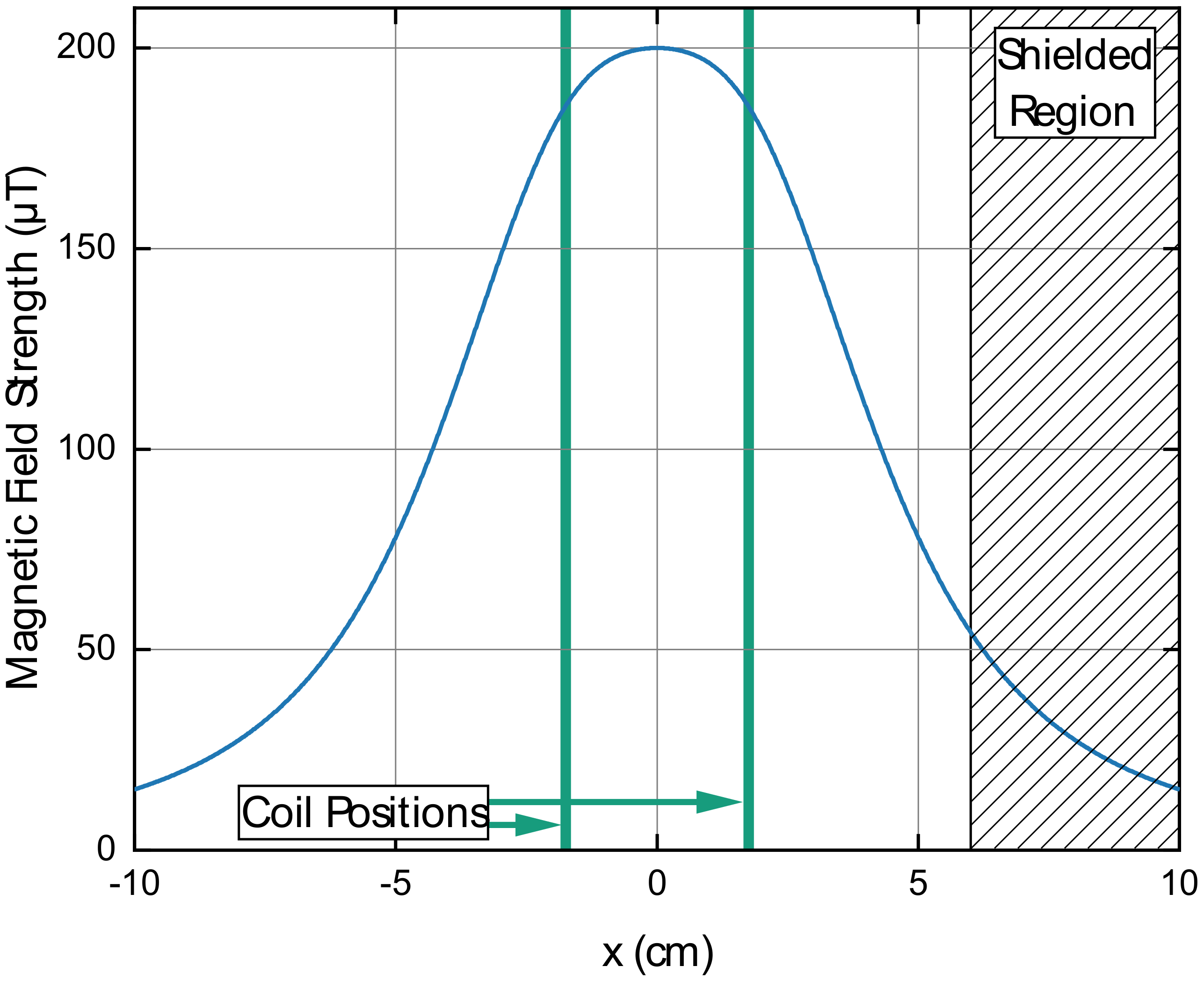
is calculated using the Biot–Savart approach for the magnetic field along the symmetric axis of the Helmholtz coils:
is the vacuum permeability,
the number of coil windings of each coil,
the electric current created by the RF voltage,
the coil radius and
the distance between the coils.
is shown in
Figure 7 for a range of ±10 cm from the coil center. Due to the geometric situation of the setup, the outer layer of the magnetic shield has approximately 6 cm from the center of the Helmholtz coil (see the shaded area in
Figure 7). For this reason, the
field distribution according to (8) shall only be considered a simple approximation.
To make the result of
comparable to experimental OPM data, the spatial distribution was converted to a temporal distribution
. This was done by converting the starting point argument
to the time
t it takes for the water to arrive in front of the OPM sensor:
.
is the distance between the RF coil and the OPM (cf.
Figure 1).
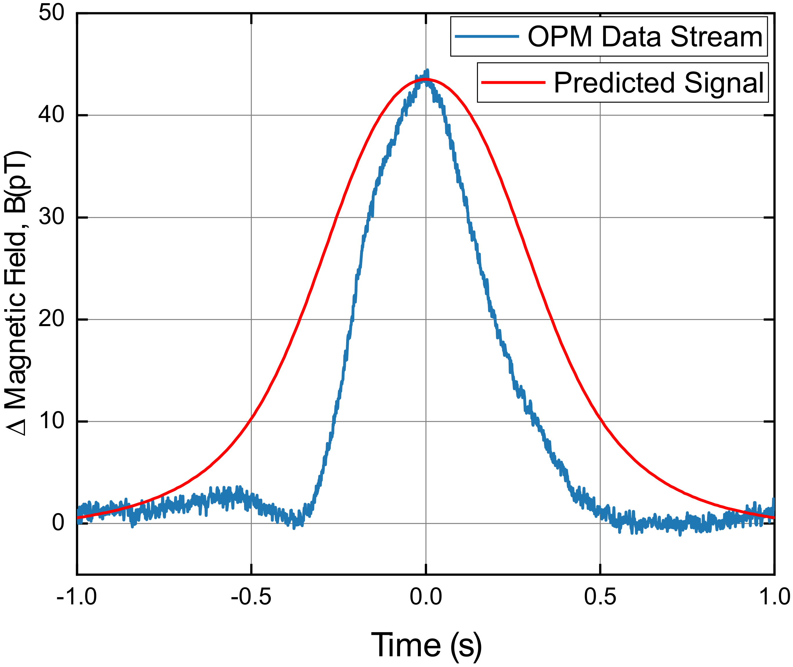
The resulting expected signal according to (7) and an extract from the experimental data are shown in
Figure 8 for comparison. For both curves the x axis was centered at t = 0. The y axis of the modeled signal was rescaled to match the peak height of the observed pulse. While the observed polarization “pulse width” (FWHM = 0.34 s) was longer than the duration of the applied RF pulse (0.25 s), it was clearly shorter than the width derived from our simple model (0.67 s). This, as well as the asymmetry of the observed “pulse” shape, indicates that the assumed B field distribution along the x axis may considerably differ from our simple model assumption.
4. Conclusions
We presented a noninvasive, magnetic-marking-based flow metering procedure, which uses an OPM operating in the ZULF regime at magnetic-field strengths lower than 100 nT as the signal detector. The detection method was based on a time-of-flight measurement, which makes the procedure calibration-free.
In the frame of the experiments, a macroscopic polarization of 300 pT was created in the water samples using a 1 T Halbach magnet. Applying short RF pulses as “markers” on the water flow resulted in polarization transients with amplitudes between 10 and 80 pT, which were detected with the OPM with good signal-to-noise ratio and used to derive the flow velocity of the medium.
In the current demonstration setup, the useful flow velocities ranged between 12.7 cm/s and 23.3 cm/s. Utilizing the procedure presented, we successfully demonstrated measuring the water flow with an average accuracy of 3% in the given velocity interval. Comparing the measured results to the pump rates of the syringe pump showed that the data were consistent with expected values.
The current experiments demonstrate the feasibility of a marker-free magnetometry-based flow metering, enabled by the outstanding performance of commercially available optically pumped magnetometers. A number of steps will be necessary to move from our “proof-of-concept” experiment to a metering system applicable in practical situations by answering the following questions:
What signals are still detectable in a certain background situation? How much shielding effort is required? Which level of pre-polarization and RF pulsing is required? What is the resulting time accuracy? What RF pulse form is best suited?
The mentioned aspects must not be considered isolated from each other. Addressing them is the topic of experiments currently under way.
Author Contributions
L.S., P.A.K. and A.L. conceptualized the research. L.S. conceived the initial idea of the procedure, performed the experiments, and wrote a draft version of the manuscript. P.A.K. and L.S. designed the experimental setup. All authors analyzed the data and revised the final version of the manuscript. All authors have read and agreed to the published version of the manuscript.
Funding
This work was supported as a Fraunhofer LIGHTHOUSE PROJECT (QMag). In equal parts, this work was funded by the Ministry of Economic Affairs, Labour and Housing of the State of Baden-Württemberg, Germany.
Data Availability Statement
The data is available from the corresponding author upon reasonable request.
Acknowledgments
We acknowledge Michael Bock of the Medical Centre of Freiburg, Germany for his helpful discussions on this research.
Conflicts of Interest
The authors declare no conflict of interest.
References
- Endress + Hauser. Flow Measuring Technology for Liquids, Gases and Steam. Available online: https://portal.endress.com/wa001/dla/5000192/0856/000/02/FA00005DEN_1918.pdf (accessed on 30 November 2021).
- Bilgic, A.M.; Kunze, J.W.; Stegemann, V.; Zoeteweij, M.; Hogendoorn, J. (Eds.) Multiphase Flow Metering with Nuclear Magnetic Resonance Spectroscopy; AMA Service GmbH: Wunstorf, Germany, 2015; p. 6. [Google Scholar]
- Thorn, R.; Johansen, G.A.; Hjertaker, B.T. Three-phase flow measurement in the petroleum industry. Meas. Sci. Technol. 2013, 24, 12003. [Google Scholar] [CrossRef]
- Halbach, R.E.; Salles-Cunha, S.; Battocletti, J.H.; Sances, A.; Bernhard, V.M. Noninvasive measurement of arterial blood flow by means of a nuclear magnetic resonance flowmeter. Surg. Forum 1978, 29, 220–222. [Google Scholar]
- Caprihan, A.; Fukushima, E. Flow Measurements by NMR. Phys. Rep. 1990, 198, 195–235. [Google Scholar]
- Falcone, G.; Hewitt, G.F.; Alimonti, C.; Harrison, B. Multiphase flow metering: Current trends and future developments. J. Pet. Technol. 2002, 54, 77–84. [Google Scholar]
- Kraus, R.H.; Espy, M.A.; Magnelind, P.E.; Volegov, P.L. Ultra-Low Field Nuclear Magnetic Resonance: A New MRI Regime; Oxford University Press: New York, NY, USA, 2014; ISBN 978-0-19-979643-4. [Google Scholar]
- Ganssle, P.J.; Shin, H.D.; Seltzer, S.J.; Bajaj, V.S.; Ledbetter, M.P.; Budker, D.; Knappe, S.; Kitching, J.; Pines, A. Ultra-Low-Field NMR Relaxation and Diffusion Measurements Using an Optical Magnetometer. Angew. Chem. Int. Ed Engl. 2014, 53, 9766–9770. [Google Scholar] [CrossRef]
- Fridjonsson, E.O.; Creber, S.A.; Vrouwenvelder, J.S.; Johns, M.L. Magnetic resonance signal moment determination using the Earth’s magnetic field. J. Magn. Reson. 2015, 252, 145–150. [Google Scholar] [CrossRef]
- O’Neill, K.T.; Klotz, A.; Stanwix, P.L.; Fridjonsson, E.O.; Johns, M.L. Quantitative multiphase flow characterisation using an Earth’s field NMR flow meter. Flow Meas. Instrum. 2017, 58, 104–111. [Google Scholar] [CrossRef]
- Fridjonsson, E.O.; Stanwix, P.L.; Johns, M.L. Earth’s field NMR flow meter: Preliminary quantitative measurements. J. Magn. Reson. 2014, 245, 110–115. [Google Scholar] [CrossRef]
- Greenberg, Y.S. Application of superconducting quantum interference devices to nuclear magnetic resonance. Rev. Mod. Phys. 1998, 70, 175–222. [Google Scholar] [CrossRef]
- Shah, V.K.; Wakai, R.T. A compact, high performance atomic magnetometer for biomedical applications. Phys. Med. Biol. 2013, 58, 8153–8161. [Google Scholar] [CrossRef] [Green Version]
- Budker, D.; Romalis, M. Optical magnetometry. Nat. Phys. 2007, 3, 227–234. [Google Scholar] [CrossRef] [Green Version]
- Guío-Pérez, D.C.; Dietrich, F.; Ferreira Cala, J.N.; Pröll, T.; Hofbauer, H. Estimation of solids circulation rate through magnetic tracer tests. Powder Technol. 2017, 316, 650–657. [Google Scholar] [CrossRef]
| Publisher’s Note: MDPI stays neutral with regard to jurisdictional claims in published maps and institutional affiliations. |
© 2022 by the authors. Licensee MDPI, Basel, Switzerland. This article is an open access article distributed under the terms and conditions of the Creative Commons Attribution (CC BY) license (https://creativecommons.org/licenses/by/4.0/).


