Utilization of Unsupervised Machine Learning for Detection of Duct Voids inside PSC Box Girder Bridges

Abstract

The PSC box girder bridge is a pre-stressed box girder bridge that accounts for a considerable part of large-scale bridges. However, when concrete is poured, even small mistakes might result in voids that appear during long-term maintenance. In this paper, we present a technique for detecting the void in the duct inside the PSC box girder bridge. Data are acquired utilizing the non-destructive impact-echo (IE) approach to detect these voids. IE creates time-series data as signal data initially; however, we want to use a CNN auto-encoder (AE). A scalogram, which is a kind of wavelet transformation, is used to convert time series data into an image. An AE is a type of unsupervised learning that aims to minimize the difference between the input and output. By comparing histograms, the difference is calculated. To begin, we create scalogram images from all IE signal data, which were randomly sampled as 98% normal and 2% void. The CNN AE is then trained and evaluated utilizing all the data. Finally, we examine the input and output histogram similarity distributions. As a consequence, only 4% of the normal data had a similarity of less than two standard deviations from the mean, whereas 34.7% of the void data did. As a result, the existence of voids inside the PSC duct could be demonstrated to be predictive in the absence of annotated data.

1. Introduction

Concrete has a high compressive strength but a low flexural strength. Pre-stressed concrete (PSC) is a type of concrete that was created to compensate for these shortcomings. PSC box girder bridges account for more than 90% of all high-speed railway bridges built to date, making them the most often used bridge type. As a result, if the PSC box girder bridge is appropriately constructed, the national SOC project cost may be reduced [1]. However, because the inner diameter of the duct is so tiny, when concrete is poured immediately on site, the construction precision may be reduced. A void inside the duct may also appear if the girder bridge is maintained for an extended period of time. Internal exploration work to verify the stability of the PSC box girder bridge is crucial in order to avoid this.

The impact-echo (IE) method, which is a non-destructive test, is used to detect voids in concrete. This method uses vibration induced by a short-term mechanical shock to determine if an object is defective. However, even if the signal is interpreted based on professional academic knowledge, it is difficult to find the signal rules; therefore, exact classification is limited. To address this issue, numerous signal classification methods have been developed. In [2], the statistical moments of the signal phase were used to automatically classify the kind of signal. The use of sparse signal representation for signal classification is also mentioned [3]. Deep learning methods have recently attracted much attention. Research was carried out using CNN, a deep learning approach for multi-signal classification [4]. They presented LSTM deep learning techniques in [5] to increase the electroglottograph (EGG) signal classification accuracy.

We propose a deep learning approach for detecting the normality and voids inside the PSC box girder bridge’s duct. We utilized an auto-encoder (AE), a type of unsupervised learning, because the signal pattern varies according on the environment in which the IE is measured. The method of existing papers is to detect data from the specimen, where the correct answer is determined. For practical application, unless checking directly into the object, the correct answer is never obtained. Therefore, unsupervised learning is applied for this purpose. Under the assumption that there is no correct answer, the goal of this paper is to determine how the data distribution between normal and void data is composed. This study differs from previous studies in that it takes a novel method.

In this study, we apply a CNN to an auto-encoder in order to transform IE signal data into images and to detect voids, which is unsupervised learning. The method of converting into an image utilizes a scalogram, which is a type of wavelet transformation. In addition, the difference between the input and output images of AE is estimated as the difference between each histogram. Finally, voids in the duct inside the PSC are detected by using the histogram similarity distribution of each image data. AE is trained using 98% randomly sampled normal data and 2% randomly collected void data. The results are assessed with the crucial assumption that the histogram similarity of normal data is greater than that of void data. As a consequence, it was determined that only 4% of the normal data differed by more than two standard deviations from the similarity mean, but 34.7% of the void data differed by more than two standard deviations. We offer a technique for detecting faults using solely unlabeled IE data in ths study.

The second section introduces previous research instances relevant to this subject. Section 3 includes a discussion of the box girder bridge, as well as an explanation of IE. The learning and prediction model proposed in this study is described in Section 4, and the experimental results of using this model are described in Section 5. Finally, the conclusion is delivered in Section 6, with a future plan.

2. Related Work

2.1. CNN AE Method for PSC Box Girder Bridges

The following study is related to recognizing the corrosion of PSC box girder bridges. In [6], a deep learning approach for determining whether damage exists is presented in order to ensure the stability of the tendon, which is the most crucial component of the PSC bridge. They predict the severity of damage using simulated data from nine accelerometers and a convolutional auto-encoder (CAE). However, this approach has a restriction of only employing an indirect signal because the damage is assessed by putting an acceleration sensor on the bridge and monitoring the difference in shaking when a vehicle passes. For this reason, it displays substantial outcomes only when the damage is very serious.

2.2. AE Methods for Anomaly Detection

Due to the fact that defects are rare, the auto-encoder, which is an unsupervised learning method, has lately been widely employed to identify them. Since it is difficult to identify the defect features in the vibration signal of a rotating machine in real time, a deep learning approach with a deep auto-encoder (DAE) is proposed in [7]. The approach is used to diagnose faults in electric locomotives. In addition, a technique for detecting wind turbine (WT) faults is presented in [8]. As a result of the uncertainty and temporal dependency of the measurement noise, the WT employs a denoising auto-encoder (DAE) to detect defects. Therefore, the auto-encoder is utilized to detect faults in a variety of areas.

Failure detection and diagnosis are critical components in ensuring the safety of industrial processes. In [9], they use an auto-encoder to detect rare faults and long short-term memory (LSTM) to identify various types of faults. The auto-encoder is trained with normal data before being used to detect anomalies, and the predicted defect data are utilized to determine the defect type using LSTM. In [10], a simulation using electrical impulses to determine normality and defects is used. In addition, in [11], a LSTM model is used to detect cavities in impact-echo time series data acquired by non-destructive testing.

2.3. Non-Destructive Testing

Many defects appear in electrical equipment, transportation systems, and other areas. Non-destructive testing methods could help in the investigation of various defects related to these issues. The impact-echo method was used for the nondestructive testing of concrete on laboratory specimens with artificial faults at known locations [12]. In addition, acoustic emission was also utilized to identify early corrosion in pre-stressed concrete girders. Acoustic emission can identify the start of corrosion in the same amount of time as traditional electrochemical approaches. It can also distinguish between different levels of corrosion [13]. These are only a few examples of non-destructive testing methods. Visual inspection, penetrant and chemical testing, nuclear radiation, acoustic and ultrasonic, thermal and microwave, and magnetic and electromagnetic procedures were all described in [14].

3. Materials

3.1. PSC Box Girder Bridge

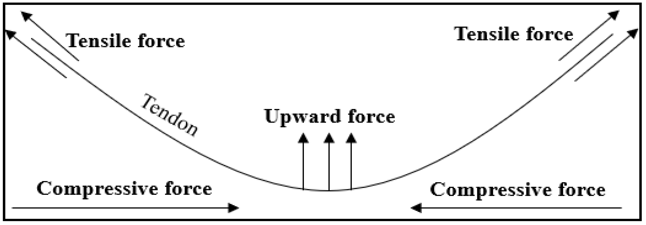
As shown in Figure 1, a compressive stress operates on the concrete when a tendon is inserted into it and strongly pulled to fix it. At this point, the tendon must be placed into the duct to avoid corrosion, and the upward force is created by the tendon’s tensile force. As a result, concrete with high bending stress is formed.

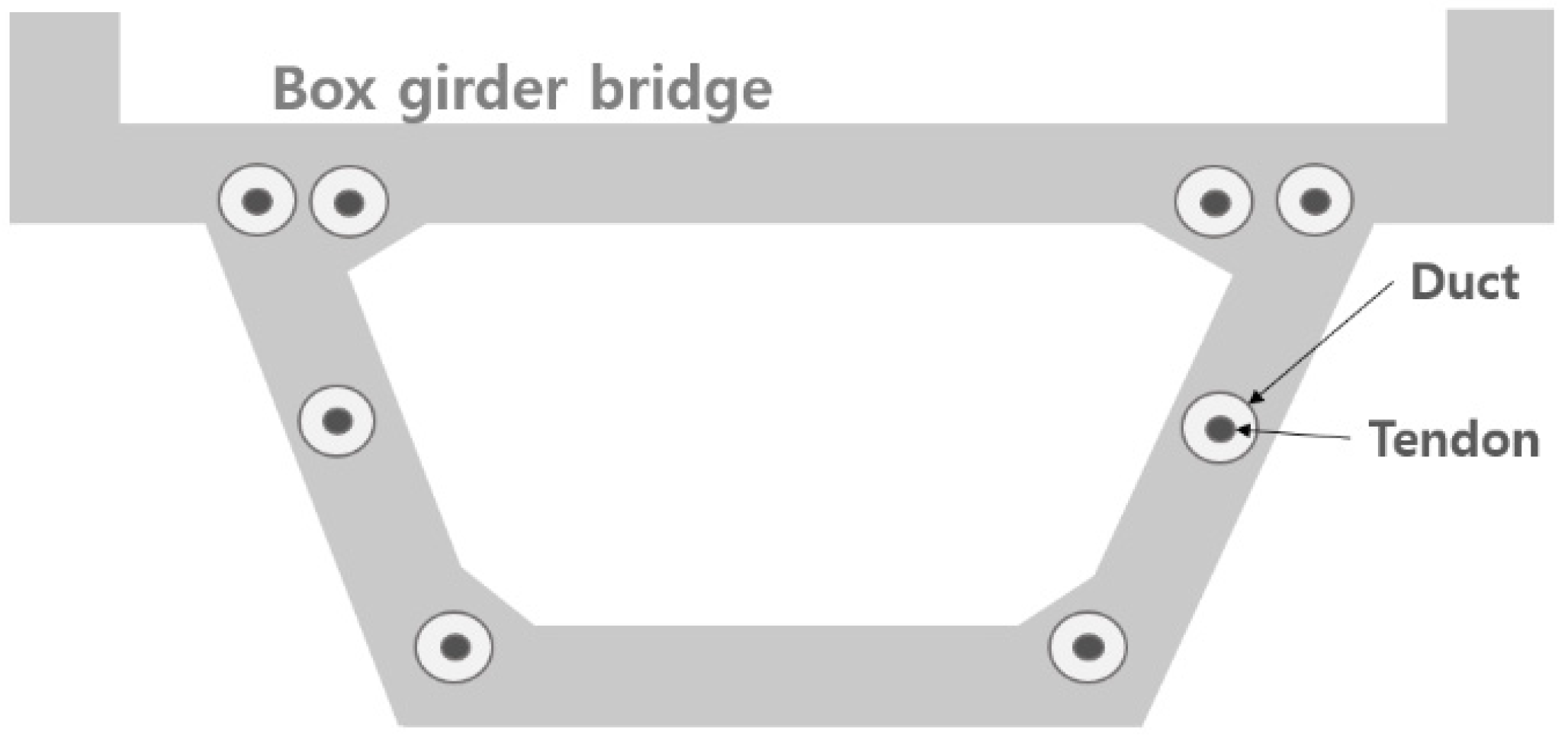
Figure 2 shows a cross-sectional view of a PSC box girder bridge. It represents an example of ducts and tendons placed into a box girder bridge. To build such a strong and safe bridge, ducts and tendons must be installed at the following areas. In addition, to prevent corrosion, the tendon must be inserted into the duct.

3.2. PSC Structure Specimen

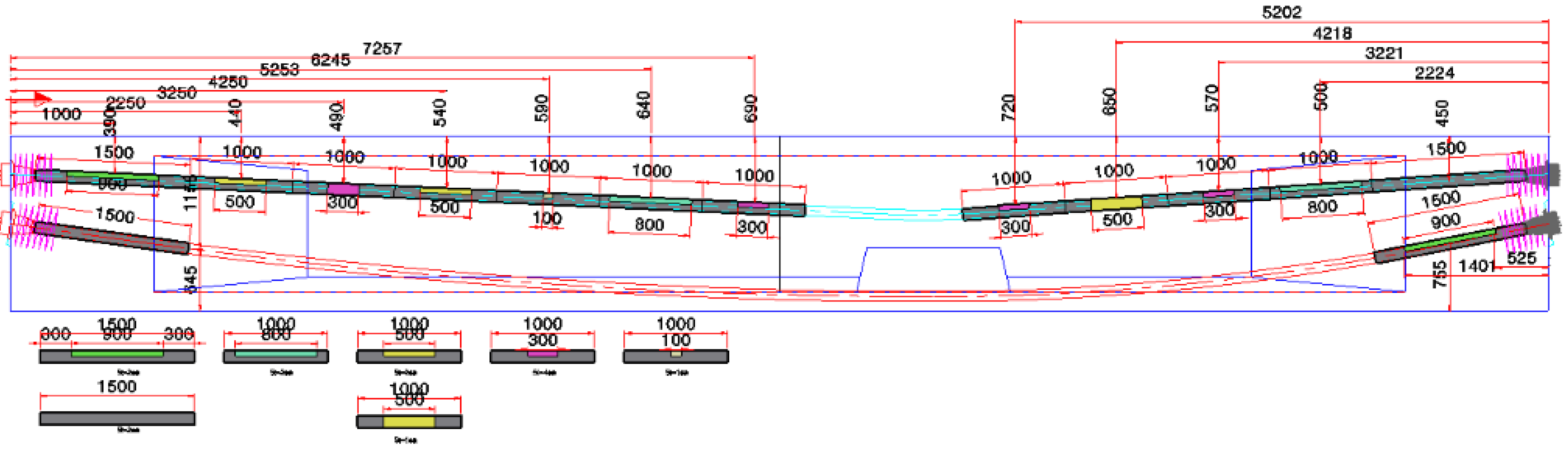
A test specimen was built with the same construction as the actual PSC box girder bridge. IE signals were collected from the test specimen for this study. As shown in Figure 3, this is the test specimen designed for multi-purpose application. The numbers represent millimeters and represent the thickness of each specimen. For each thickness, IE signals with normal and void structure are collected.

In the following specimen structure, the parts painted with different colors represent the parts with voids. As shown in the lower left figure, each part where the void was designed was built separately, and the entire pipe was connected. It is manufactured in various types based on the size of the void, and is distinguished by different colors. The number of produced duct tubes is indicated beneath each designed duct tube. The numbers on the red line above represent the distance from the start and end to the center of the void and the distance to the concrete surface. The thickness is defined as the distance between the void of the duct pipe and the concrete surface, and signal data measured at various thicknesses are employed.

The concrete surface in the center of the duct with the void serves as the void data measuring point. We measure in a position positioned vertically in the center of the colored specimen. Normal data are collected on concrete surfaces that do not match the void specimens created. The signal used in this study was measured at a thickness of 250 to 280 mm. They use 1253 random samples (98% of the normal data) and 23 random samples (2% of the void data). The goal is to use these relevant data for the detection of voids in actual PSC bridges.

3.3. Impact-Echo

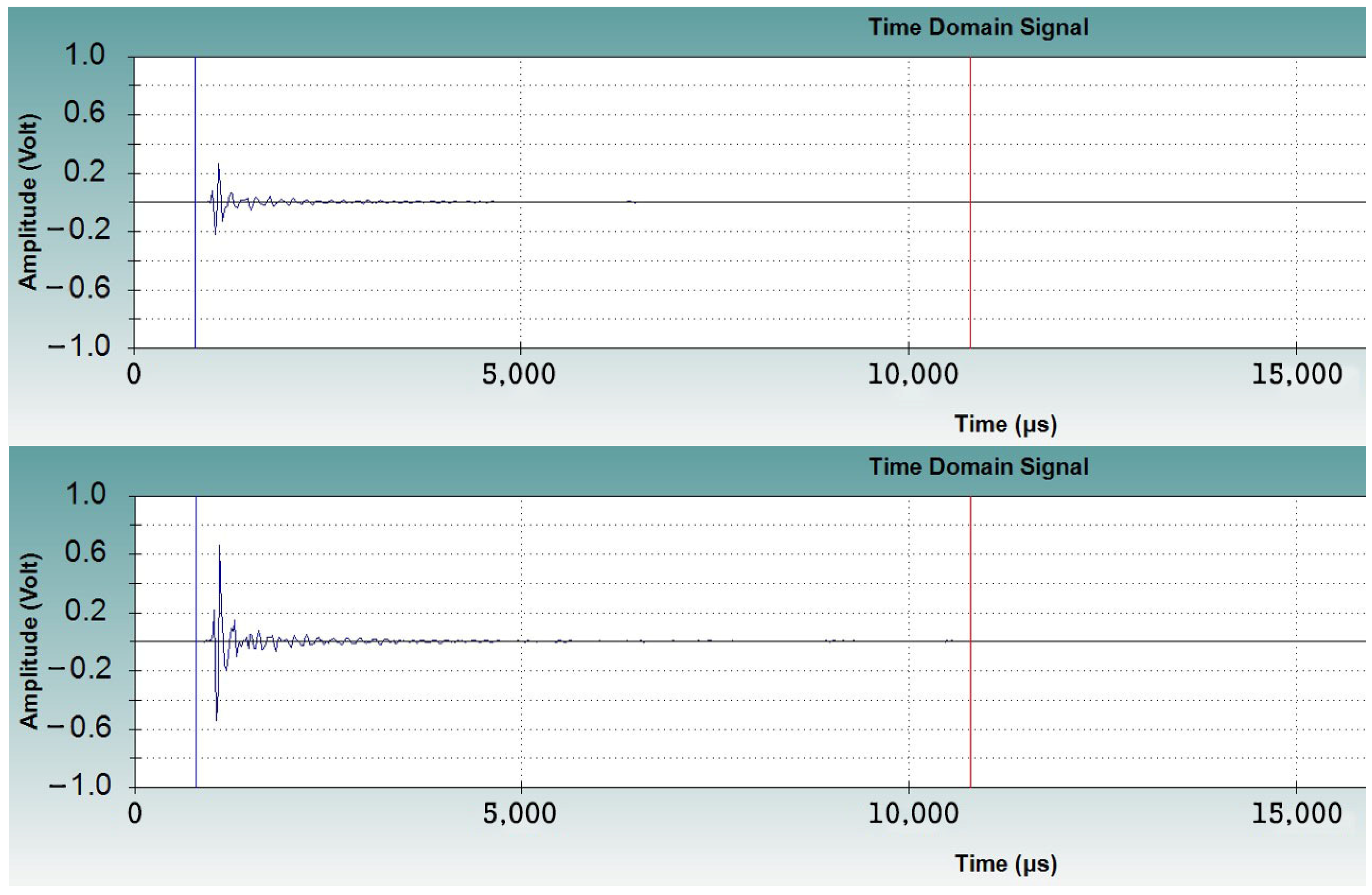
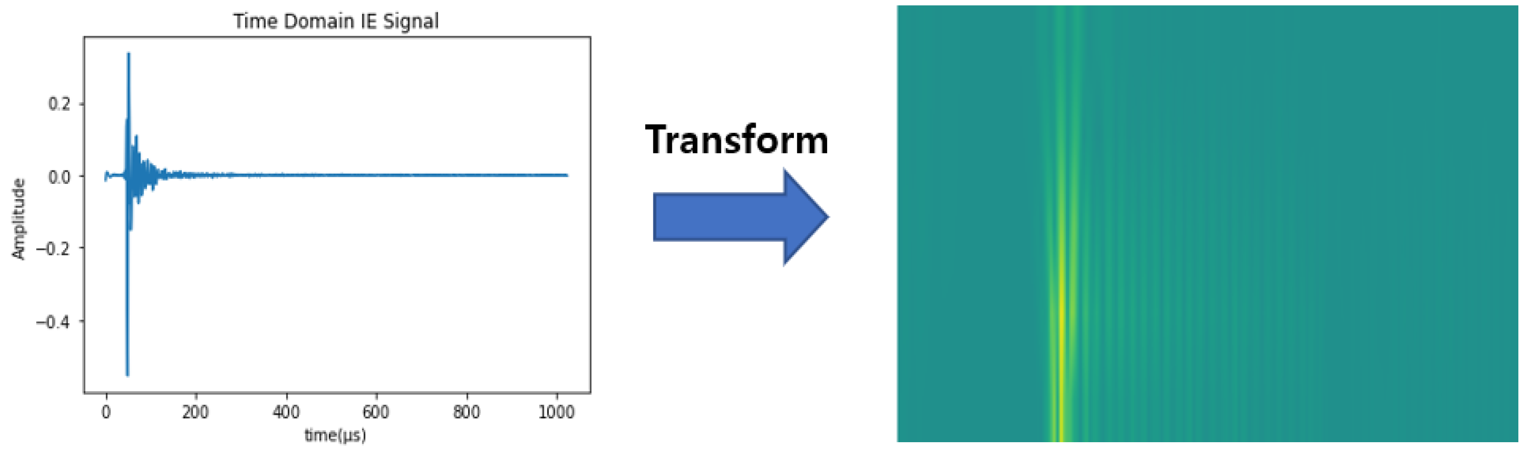
The impact-echo (IE), a non-destructive test method, is used to detect voids inside the specimen’s duct. Figure 4 is an example of an IE signal with a normal and void structure. This approach generates signal data based on surface motion caused by a short-term mechanical impact. It is related to the shape of the object to be identified and the presence of defects, since each void creates distinct vibrations [15]. As indicated in Figure 5, relevant signals with a length of 0–1024 $\mathsf{\mu }\mathrm{s}$ were used in this study, and, depending on the situation, the raw signals were pre-processed by filtering using low-pass and high-pass filters.

4. Methodology

In this study, IE signal data from test specimens were applied to CNN. Time series data were converted into a scalogram image for this purpose. After that, it was put into the CNN auto-encoder, and the input and output images were compared and analyzed. The histogram similarity was used to calculate the difference between the two. Training and test data accounted for 98 % of normal data and 2% of void data. The smaller the histogram similarity, the higher the probability of void data, and this paper evaluates its performance.

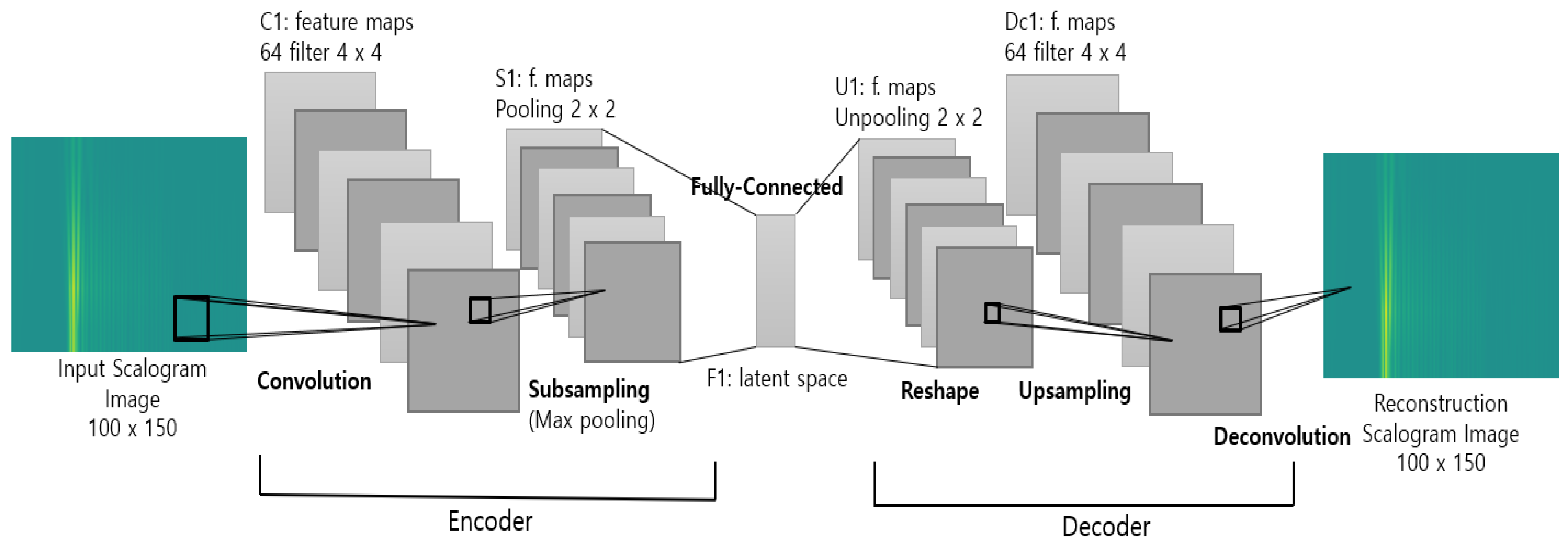
The converted scalogram image was inserted into the CNN auto-encoder model. Figure 5 shows the model structure, which is simple. The encoder consisted of a convolution layer and a sub-sampling (max pooling) layer, whereas the decoder consisted of an up-sampling layer and a de-convolution layer. The convolution layer was calculated using a filter and a convolution operation, and the max pooling layer extracted the maximum value of the filter values. Latent space is a latent feature that was flattened and fully connected. The decoder’s up-sampling and de-convolution converted this latent representation back into an image. The CNN AE reconstructed the input scalogram image into an output scalogram image throughout this process.

4.1. Scalogram Transform

To effectively apply time series data to CNN, the signal should be converted into an image. Wavelet theory has proven to be a useful tool for studying time series. The two parameters of the continuous wavelet transform (CWT) (time $u$ and scale $s$) allow for simultaneous signal analysis in two domains (time and frequency). The time–frequency decomposition was provided by the $f$ of the CWT in the time–frequency plane.

Through time $u$ and scale $s$, CWT provided decomposition in the time–frequency domain. Scale can be used to optimize scalograms in the time–frequency area if this method is used. We can examine the similar patterns that exist between each scalogram image by transforming each time series in this way, as shown in Figure 6.

$$S\left(s\right) :=\parallel Wf\left(s,u\right)\parallel ={\left({{\displaystyle \int }}_{-\infty }^{\infty }{\left|Wf\left(s,u\right)\right|}^{2}du\right)}^{\frac{1}{2}}$$

(1)

The function of the scalogram is defined as the $Wf$ function, which represents the energy at the scale $s$, as shown in Equation (1). It must be $S\left(s\right)$ ≥ 0 for all scales $s$, and if $S\left(s\right)$ > 0, the signal $f$ has details at scale $s$ [16]. Therefore, using a scalogram, most representative scale (or frequency) of the signal can be determined, i.e., the scale that contributes the most to the total energy of the signal. In this study, the image was transformed by setting the value of scale s to 1–5. Furthermore, useless sections of the original IE signal were eliminated, and only signals matching to 0–192 μs were translated into images.

4.2. Other Image Transform Methods

In addition to the scalogram transformation used in this paper, there were GAF (Gramian angular fields) and MTF (Markov transition fields) [17] imaging methods. There was also a method that used recurrence plots (RP), which is a plot imaged using the distance between points located on each spatial trajectory after drawing time series data on an m-dimensional spatial trajectory [18].

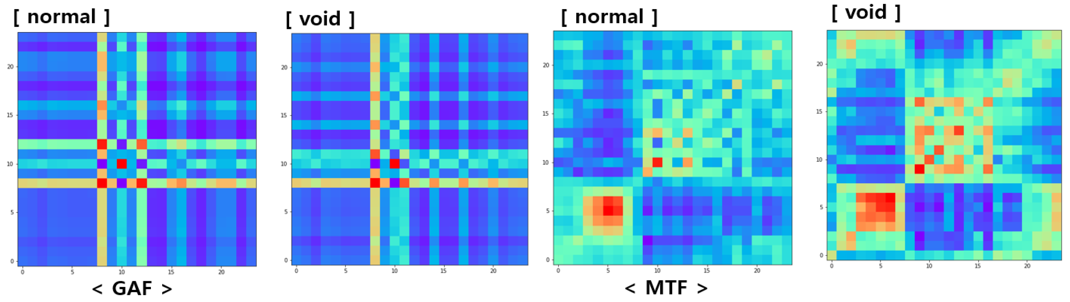
GAF is an algorithm that uses polar coordinates to represent the temporal correlation between time-steps. Time moves from top left to bottom right in this approach, maintaining time dependency. MTF is an algorithm that expresses the transition probability of discrete time series data. It divides a given time series dataset into multiple intervals and constructs a weighted adjacency matrix along the time axis using a linear Markov chain. To avoid information loss, it sorts each probability in chronological sequence. As shown in Figure 7, we tried to convert images using these methods and apply them to the CNN auto-encoder, but it was difficult to distinguish between normal and void data. In this study, the scalogram transformation was able to better distinguish the features of the signal. This will be mentioned in the Results.

4.3. CNN (Convolutional Neural Network)

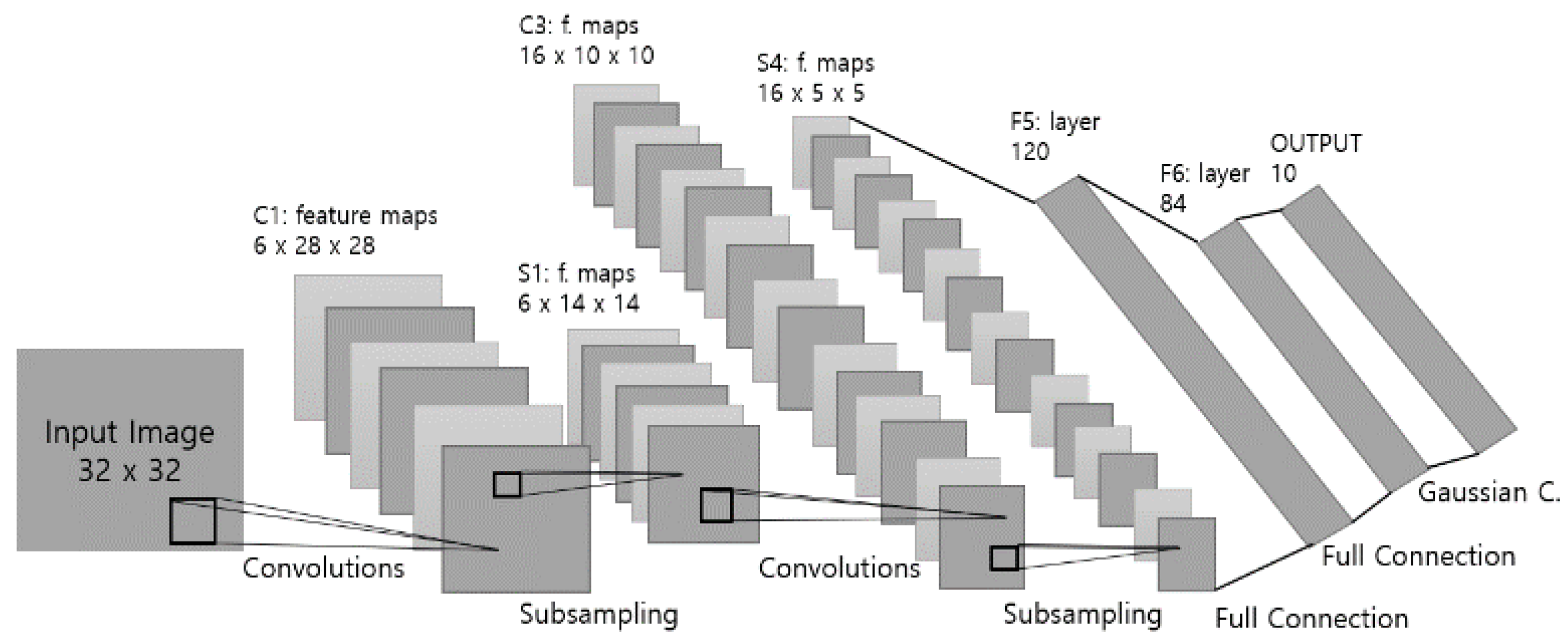
Convolutional neural network (CNN) is an essential component of deep learning in image processing and is used in computer vision. Convolution layers, pooling layers, and fully connected layers are examples of layer types. The convolution layer, which is composed of many feature maps, is trained to express the features of the input data. The convolutional results are then transferred to non-linear activation functions, such as Relu and sigmoid. By reducing the size of the feature map, the pooling layer extracts secondary features and promotes robustness. Average pooling and max pooling are some common techniques. The fully connected layer combines every neuron from the previous layer to every neuron in the current layer. The output layer is formed after the last fully connected layer. Figure 8 shows a visualization of the CNN model, and [19] is referenced.

$$\left(f\ast g\right)\left(t\right)={{\displaystyle \int }}_{-\infty }^{\infty }f\left(r\right)g\left(t-r\right)dr$$

(2)

The convolution operation is represented in Equation (2), and the shape of the function $f$ generates a function ($f\ast g$) whose shape is modified by the remaining function $g$. $f$ and $g$ refer to the image and the filter, respectively, and this expression is equivalent to the integral of the function $f\left(r\right)$ multiplied by $g\left(t-r\right)$. This means that one of the two functions is inverted for the convolution operation process, and the filter $g$ is shifted by $t$.

4.4. Auto-Encoder

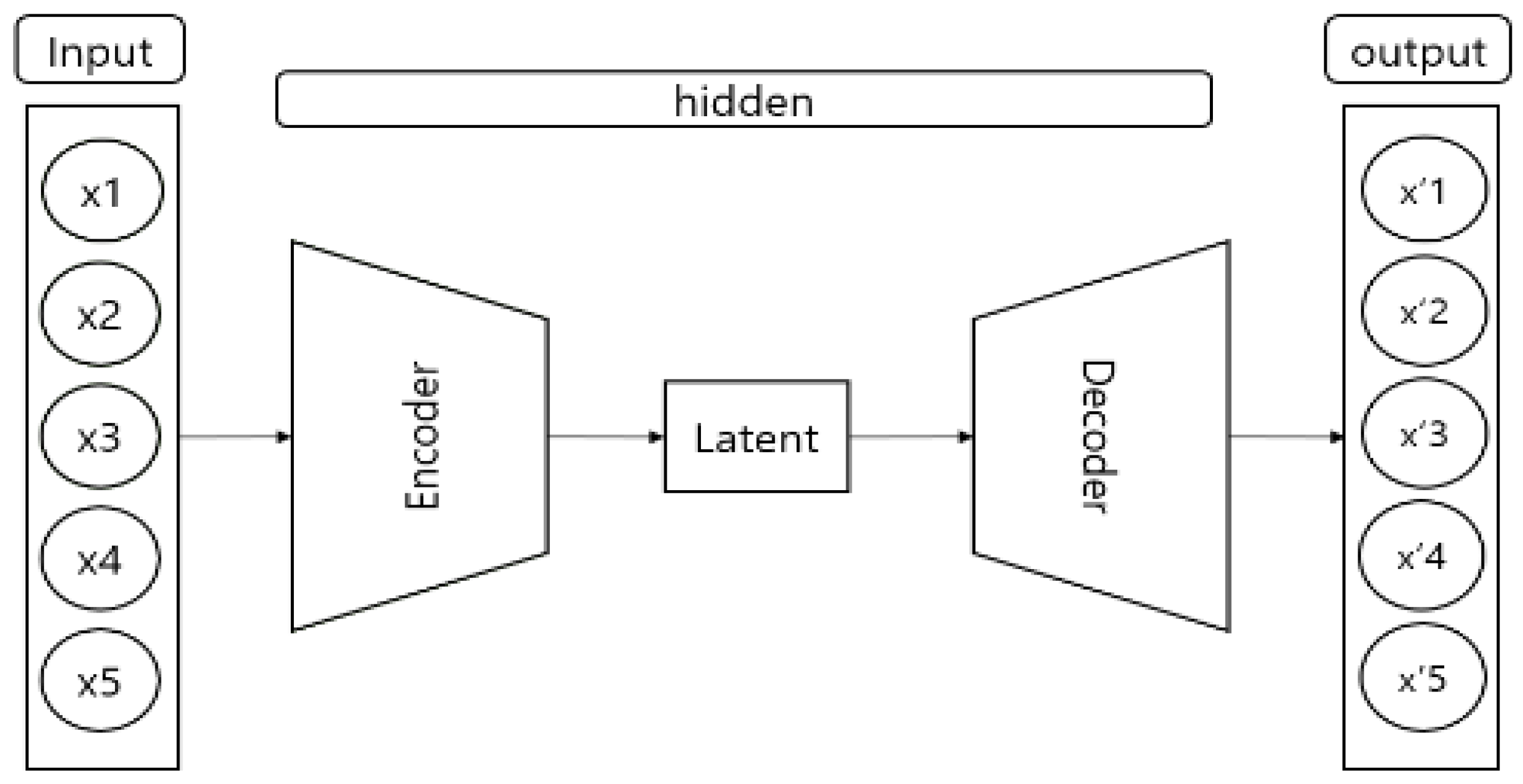
The auto-encoder is an artificial neural network (ANN) with three sequentially connected layers: input, hidden, and output layers. In addition, it is an unsupervised learning method [20], as shown in Figure 9. The training procedure consists of an encoder that maps the input data to the hidden layer and a decoder that reconstructs the input data. The difference between the input data and the reconstructed output data are referred to as a reconstruction error, and a model is trained to minimize this error. In this paper, the convolutional network was applied to the encoder and decoder of auto-encoder.

4.5. Histogram Similarity

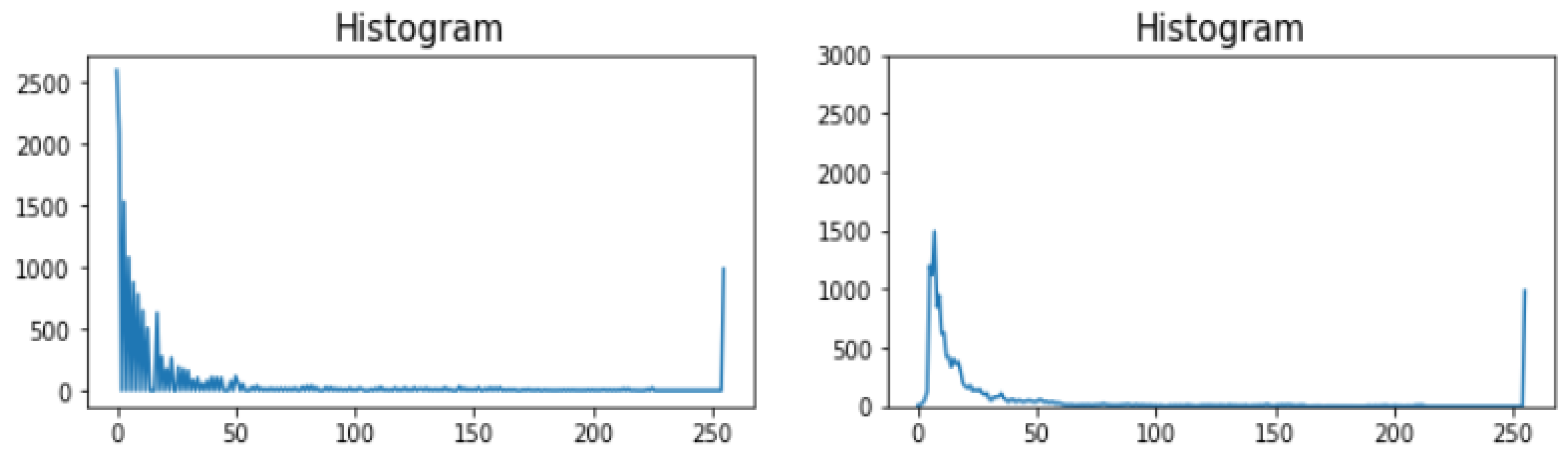
Finally, the histogram distribution of the original scalogram was compared with the histogram distribution of the reconstructed scalogram from CNN AE. At this point, the histogram similarity of the two was calculated using the Opencv library’s CompareHist() function.

$$d\left(H_1,H_2\right)=\frac{{\sum }_I\left(H_1\left(I\right)-{\overline{H}}_1\right)\left(H_2\left(I\right)-{\overline{H}}_2\right) }{\sqrt{{\sum }_I{\left(H_1\left(I\right)-{\overline{H}}_1\right)}^2{\sum }_I{\left(H_2\left(I\right)-{\overline{H}}_2\right)}^2}}$$

(3)

$${\overline{H}}_k=\frac{1}{N}{\displaystyle \sum }_J{H}_k\left(J\right)$$

(4)

It was performed using Opencv’s correlation theory, and the calculation formula is Equation (3). It is a number between 0 and 1, and the greater the number, the closer the pair are to each other. In Equation (4), N is the total number of histogram bins. As shown in Figure 10, the left graph represents the histogram distribution of the original image, whereas the right graph represents the histogram distribution of the reconstructed image. In the following example, the histogram similarity is 0.6412.

5. Results

The data are made of 98% randomly sampled data (1253) from a normal specimen and 2% randomly sampled data (23) from a specimen with voids in the duct. All of these data are converted into a scalogram image and used to train and test the CNN auto-encoder. When the image data of the PSC specimen’s internal duct are put into the CNN AE, the results show the normal and void distribution as the histogram similarity of the input and output, as shown in

Table 1. Distribution of normal and void data in the duct. In the histogram similarity distribution, the boundaries are set as mean, mean–standard deviation (−σ), and mean–2 × standard deviation (−2σ).

Boundary	Higher/Lower	Normal Num (Ratio)	Void Num (Ratio)
Mean	Higher	693/1253 (55.3%)	4/23 (17.3%)
	Lower	560/1253 (44.6%)	19/23 (82.6%)
Mean–Standard deviation	Higher	1089/1253 (86.9%)	12/23 (52.1%)
	Lower	164/1253 (13%)	11/23 (47.8%)
Mean–2×Standard deviation	Higher	1202/1253 (95.9%)	15/23 (65.2%)
	Lower	51/1253 (4%)	8/23 (34.7%)

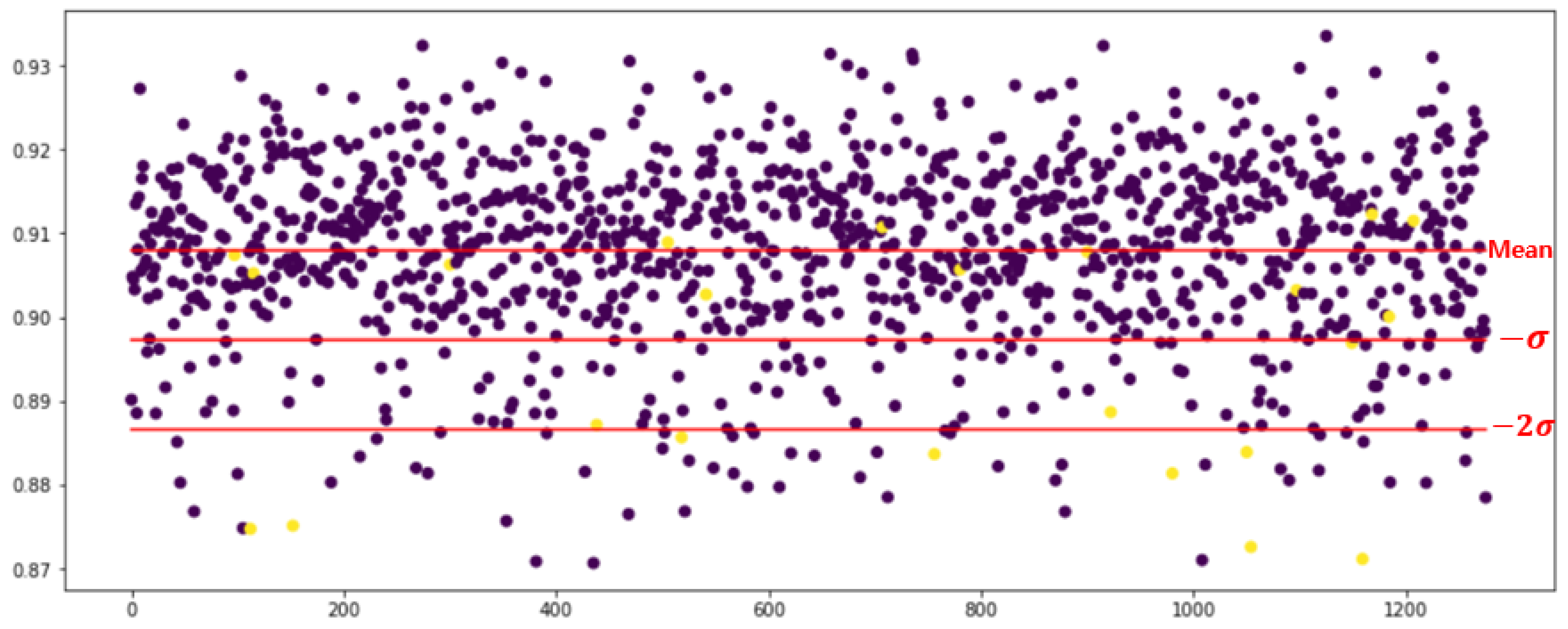
. Figure 11 shows the visual plot. The boundaries of the similarity distribution are Average, Avg-Std (−σ), and Avg-2*Std (−2σ). As a result, we compare the distribution of data with high similarity and low similarity to the boundary line.

First, we examine the distribution with the mean as the boundary. The proportion of data with a histogram similarity higher than the mean is 17.3% for void data and 55.3% for normal data. In comparison to the normal data, where the ratio of the data less than the mean is 44.6%, the void data occupies most, at 82.6%. When comparing data distributions based on mean–standard deviation—that is, −σ—data distributions higher than the boundary are 86.9% normal. In the case of data that have a lower similarity than the boundary, the normal data have a distribution with a ratio of 13%, but the void data have a distribution with a ratio of 47.8%.

Finally, when comparing data on the mean–2×standard deviation boundary—that is, −2σ—data over the boundary have a normal ratio of 95.9%. Furthermore, for data with a histogram similarity lower than the boundary, it is confirmed that the normal data have a ratio of 4% and the void data ratio is 34.7%. The normal ratio is much larger than the void ratio for data above the boundary, whereas the void ratio is much larger than the normal ratio for data below the boundary. As a conclusion, the overall distribution indicates that the histogram similarity of normal data is mainly high, whereas that of void data is mostly lower than that of the boundary.

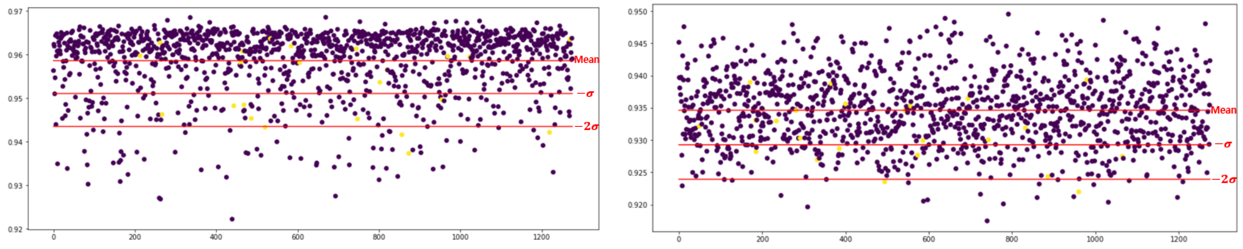
Additional experiments, on the other hand, were carried out using the GAF and MTF methods, which are the image transformation methods mentioned in Section 3.2. Other Image Transform Methods. The Compare_ssim() function of scikit-image was used to calculate the similarity between input and output images. Figure 12 shows the similarity distribution plot for the experimental results. The performance of anomaly detection was examined using the −2σ boundary. First, in the GAF experiment, the data with a lower similarity to the −2σ boundary have a distribution of normal 5% and void 17.3%. In the MTF experiment, the data with a lower similarity based on the same boundary are composed of normal 1.5% and void 8.6%. We found that this extra experiment produced no significant results when compared to the previous approach.

Meanwhile, existing methods predict the label measured through the specimen and evaluate the accuracy. However, it is difficult to predict the data measured in actual bridges with such methods. The approach of this study is to examine the data distribution by analyzing and visualizing the number of differences between the void and normal data. Although this shows a result that cannot be expressed with clear accuracy, it can be a useful metric for detecting the normal and void data of an actual bridge.

6. Conclusions

The most often used PSC box girder bridge can cause voids in the duct when concrete is poured or when it is maintained for an extended period. In this study, we propose an unsupervised CNN AE method for detecting such voids. For training, 98% of the normal data and 2% of the void data are randomly sampled. To effectively use the CNN model, the IE signal obtained from the manufactured specimen is converted into a wavelet transformed scalogram image. The purpose of AE is to reduce the difference between the input and output, and this difference is estimated utilizing histogram similarity. As a conclusion, because most of the training data are normal data, data with voids differ from normal data. When the histogram similarity distribution of each data set is compared using mean, −σ, and −2 × σ, the data above the boundary are generally normal data, whereas the data below the boundary are mostly void data. This helps in the detection of voids for actual PSC girder bridges where no correct label is given.

The difference between normal and void data was validated in this study. However, in the end, a model that can distinguish between normal or void data is required for the given data. The following study should be undertaken in the future to help with this. To begin, we want to design a pattern that can distinguish between normal and void data only when the similarity is less than a specific degree. Due to the nature of field data, a classification model based on unsupervised learning is required. Second, rather than the test specimen, actual bridge data must also be colloected. The location and severity of defects on actual bridges vary greatly. Therefore, data reflecting the diversity of real-world sectors are necessary for more precise learning.

However, this study is the first approach toward a non-teaching learning method that targets actual data rather than test specimens. It is uncertain whether the prediction will work for actual equipment and objects, even if the prediction is made with high accuracy by experimenting with simulations and test specimens, as in existing papers. As a result, the first approach in this study requires additional experiments, and is critical.

References

- Cho, K.S.; Ahn, G.E.; Lee, J.Y.; Kwak, J.W.; Kwak, I.J. Optimal Section of PSC Box Girder Railway Bridge. In Proceedings of the 11th International Symposium on STEEL STRUCTURES, Yeosu, Korea, 22–24 October 2015; pp. 172–176. (In Korean). [Google Scholar]
- Soliman, S.S.; Hsue, S.Z. Signal classification using statistical moments. IEEE Trans. Commun. 1992, 40, 908–916. [Google Scholar] [CrossRef]
- Huang, K.; Aviyente, S. Sparse representation for signal classification. Adv. Neural Inf. Process. Syst. 2006, 19, 609–616. [Google Scholar]
- Elbir, A.M. Deepmusic: Multiple signal classification via deep learning. IEEE Sens. Lett. 2020, 4, 7001004. [Google Scholar] [CrossRef] [Green Version]
- Nagabushanam, P.; Thomas George, S.; Radha, S. EEG signal classification using LSTM and improved neural network algorithms. Soft Comput. 2020, 24, 9981–10003. [Google Scholar] [CrossRef]
- Lee, K.; Jeong, S.; Sim, S.H.; Shin, D.H. A novelty detection approach for tendons of prestressed concrete bridges based on a convolutional autoencoder and acceleration data. Sensors 2019, 19, 1633. [Google Scholar] [CrossRef] [PubMed] [Green Version]
- Shao, H.; Jiang, H.; Zhao, H.; Wang, F. A novel deep autoencoder feature learning method for rotating machinery fault diagnosis. Mech. Syst. Signal Process. 2017, 95, 187–204. [Google Scholar] [CrossRef]
- Jiang, G.; Xie, P.; He, H.; Yan, J. Wind turbine fault detection using a denoising autoencoder with temporal information. IEEE/ASME Trans. Mechatron. 2017, 23, 89–100. [Google Scholar] [CrossRef]
- Park, P.; Marco, P.D.; Shin, H.; Bang, J. Fault detection and diagnosis using combined autoencoder and long short-term memory network. Sensors 2019, 19, 4612. [Google Scholar] [CrossRef] [PubMed] [Green Version]
- Lee, J.U.; Bang, S.S.; Yoon, S.H.; Shin, Y.J.; Lim, Y.J.Y.M. IOP Conference Series: Materials Science and Engineering. In Proceedings of the International Conference on Robotics and Mechantronics (ICRoM 2017), Hong Kong, China, 12–14 December 2017; Volume 12, p. 14. [Google Scholar]
- Oh, B.D.; Choi, H.; Song, H.J.; Kim, J.D.; Park, C.Y.; Kim, Y.S. Detection of Defect Inside Duct Using Recurrent Neural Networks. Sens. Mater. 2020, 32, 171–182. [Google Scholar] [CrossRef] [Green Version]
- Sansalone, M.; Carino, N.J. Impact-echo method. Concr. Int. 1988, 10, 38–46. [Google Scholar]
- ElBatanouny, M.K.; Mangual, J.; Ziehl, P.H.; Matta, F. Early corrosion detection in prestressed concrete girders using acoustic emission. J. Mater. Civ. Eng. 2014, 26, 504–511. [Google Scholar] [CrossRef]
- Bray, D.E.; McBride, D. Nondestructive testing techniques. NASA STI/Recon Tech. Rep. A 1992, 93, 17573. [Google Scholar]
- Carino, N.J. The impact-echo method: An overview. Structures 2001, 1–18. [Google Scholar] [CrossRef] [Green Version]
- Bolós, V.J.; Benítez, R. The wavelet scalogram in the study of time series. In Advances in Differential Equations and Applications; Springer: Cham, Switzerland, 2014; pp. 147–154. [Google Scholar]
- Wang, Z.; Oates, T. Imaging Time-Series to Improve Classification and Imputation. In Proceedings of the Twenty-Fourth International Joint Conference on Artificial Intelligence, Buenos Aires, Argentina, 25–31 July 2015. [Google Scholar]
- Hatami, N.; Gavet, Y.; Debayle, J. Classification of Time-Series Images Using Deep Convolutional Neural Networks. In Proceedings of the Tenth International Conference on Machine Vision (ICMV 2017), Vienna, Austria, 13–15 November 2017; International Society for Optics and Photonics: Bellingham, WA, USA, 2018; Volume 10696, p. 106960. [Google Scholar]
- LeCun, Y.; Bottou, L.; Bengio, Y.; Haffner, P. Gradient-based learning applied to document recognition. Proc. IEEE 1998, 86, 2278–2324. [Google Scholar] [CrossRef] [Green Version]
- Sagheer, A.; Kotb, M. Unsupervised pre-training of a deep LSTM-based stacked autoencoder for multivariate time series forecasting problems. Sci. Rep. 2019, 9, 19038. [Google Scholar] [CrossRef] [PubMed] [Green Version]