
The Spec-Radiation Method for Layered Fluid Media


Institute of Dynamic and Vibration Research, Leibniz University of Hannover, 30823 Garbsen, Germany
*
Author to whom correspondence should be addressed.
Appl. Sci. 2022, 12(3), 1098; https://doi.org/10.3390/app12031098
Submission received: 3 December 2021
/
Revised: 12 January 2022
/
Accepted: 17 January 2022
/
Published: 21 January 2022
(This article belongs to the Special Issue Ultrasonic Modelling for Non-destructive Testing)
Abstract
:The real-time evaluation for non-destructive air-coupled ultrasonic testing of panel materials is a big task for several industries. To make these tests more and more accurate, efficient and reliable calculation methods from ultrasonic holography are essential. In the past, we presented the spec-radiation method as a fast and accurate method for such tasks. The spec-radiation method calculates the sound field utilizing data from a measurement plane at another parallel or tilted plane, especially the sound field at the surface of a panel. This can be used to detect flaws. There is a limitation of the current method: using the data on the panel surface limits the accuracy of the detected flaws. A big step forward could be expected if the sound field in the material were known. As a first step, we developed the spec-radiation method forward to consider multiple material layers. For now, we made the major assumption that all layers have fluid-like properties. Hence, transversal waves were neglected. This extension of the spec-radiation method was validated utilizing an experiment. We present that flaws in the panel material can be detected with higher accuracy at a similar speed compared to our former approach.
1. Introduction
Today’s panel materials industry is dependent on fast, reliable, accurate, and non-destructive testing to guarantee the materials’ quality. This is because the demands on the panel material are increasing, while at the same time, material and thus costs must be saved. This affects a wide range of industries, such as wind turbine manufacturers (Jasiuniene et al. [1]), the construction industry (Conta et al. [2]), aeronautical applications (Fahr [3]), the wood-based panel industry (Fang et al. [4]), and many others. Sokolov [5] used ultrasound for the first time to test a material for defects. Shortly thereafter, Firestone developed the first echo material tester based on the reflection principle, and Trost developed an ultrasonic forceps based on ultrasonic transmission. After that, the further development of ultrasonic testing was inevitable (Deutsch et al. [6], Krautkrämer and Krautkrämer [7]).
Ultrasonic testing can be roughly divided into two groups: contact testing, in which the transmitter and receiver are in direct contact with the material to be tested, and non-contact testing, in which the ultrasonic waves are transmitted from a transmitter to the material via an ambient medium, and from there to the receiver. Ultrasonic testing with contact to the test object offers the advantage that sound energy can be transmitted easily with low losses. However, the applied contact force has an influence on the result (Gyekenyesi et al. [8]). Due to the high difference in impedance between the transmitter or receiver and the test object, a thin layer of a contact medium is often applied to further increase the sound energy. This contact medium consists in most cases of water-containing oils, gels, or fats (Willcox and Downes [9]). However, with some materials, this has the disadvantage that the contact oil leaves residues on the test object or is even absorbed by the test object (as is the case with wood-based materials, for example), thus changing the material properties of the test object (Schafer [10]). These disadvantages led to the development of non-contact ultrasonic testing (Fang et al. [4]). Non-contact ultrasonic testing is especially suitable for objects with higher temperatures in corrosive or other dangerous environments or areas that are difficult to access. It allows large distances from the structures to be tested (Green [11]), and due to the missing contact force, it cannot influence the results. Usually, water is used as the ambient medium for contactless ultrasonic testing. This is because water has good impedance properties with respect to most solid materials (Jasiuniene et al. [1], Zhang et al. [12], Mitri et al. [13]). For materials such as wood, however, testing under water is not possible because the material would absorb the water, change its properties, and/or even be destroyed. Air-coupled ultrasonic testing was developed for such materials. A major challenge is the large difference in the impedance of air compared to most solid materials. According to Stößel [14], in carbon-fiber-reinforced plastic (CFRP) plates, only 0.000004% of an incident wave is transmitted into the material; the rest is reflected, and only about 0.005% of the energy is transmitted by a piezoceramic to the air. To be able to use air-coupled ultrasonic testing successfully, the transmitters are provided with a matching layer. These are connected directly to the vibration generator (e.g., the piezoceramic) and usually have a characteristic length of a quarter of the wavelength () of the respective material of the matching layer (Chimenti [15], Álvarez Arenas [16]). The application of modern materials allows the successful use of air-coupled ultrasound (Hillger et al. [17]). Air-coupled ultrasound is currently used in a wide range of applications, e.g., for the examination of turbine blades made of glass-fiber-reinforced plastics (GFRPs) (Raisutis et al. [18]) or wood-based materials (Sanabria et al. [19]), to name a few.
During the production process of wooden particleboard, delamination, air inclusions, or insufficiently glued areas can occur (Dunky and Niemz [20]). The first who detected such flaws in wood by ultrasound were Niemz [21], Bucur and Böhnke [22]. They assessed whether delamination was present based on the change in the propagation time of the signal. If the particleboard is to be inspected during production, it usually still has a very high temperature (>100 °C) and vapors escaping, that can lead to receiver damage (Dunky and Niemz [20]). This means that the receivers must be placed at a large distance (>100 mm) from the particleboard. These large distances from the wooden particleboard make a direct detection of flaws very difficult, if not impossible, since the sound waves diffract and interfere all the way to the receiver (Laybed and Huang [23]).
According to Döring [24], the three best-known methods of presenting the information from a non-destructive test with air-coupled ultrasound are the A-, B-, and C-scans. An A-scan is the time-dependent measurement of a single point; a B-scan is a line of A-scans; a C-scan is a set of multiple B-scans. The C-scan in particular enables good detection of flaws or delaminations in shape and position, but is also the most time consuming because a large number of points must be measured.
However, as already mentioned, at greater distances from the test object, it becomes increasingly difficult to find a clear indicator for flaws due to the diffraction and interference of the sound waves. If the transmitter is stationary during the measurements and only the receiver is moved, tomographic measurements can be performed (Chimenti [15]). If, in this way, the information of a plane is measured and known, methods of acoustic holography can be applied to calculate from that plane to another plane directly above the object under test. The acoustic holography originates from the holography in optics invented by Gabor [25]. Acoustic holography enables the calculation of sound fields starting from a known plane in the sound field. Due to the coherent properties of ultrasonic waves, diffraction-induced inaccuracies can be eliminated in this way (Singh [26]). An important method of acoustic holography for the detection of flaws is the re-radiation method (Sanabria et al. [27], Marhenke et al. [28], Marhenke et al. [29], Marhenke et al. [30], Schmelt et al. [31], Schmelt et al. [32], Schmelt et al. [33]). With the re-radiation method, flaws in the sub-wavelength range can be identified (Marhenke et al. [28]). Under the assumption that the solid test object is similar to a fluid and only longitudinal waves can propagate, a well-interpretable result has already been obtained on the side facing away from the receiver (Marhenke et al. [28]), and objects in a sound field have also been determined (Schmelt et al. [31], Tsysar and Sapozhnikov [34]). The re-radiation method is based on the Rayleigh–Sommerfeld diffraction integral and thus offers a well-interpretable description in the spatial domain. Due to the description in the spatial domain, the computation effort is not low, since several two-dimensional Fourier transformations (FFTs) and inverse Fourier transformations (iFFTs) have to be performed for the evaluation. The spec-radiation method (Schmelt and Twiefel [35]) offers the possibility to perform faster computations, since the data are processed in the spatial frequency domain, so fewer FFTs and iFFTs have to be performed. The smallest detectable flaws that can be detected theoretically are, according to Wolf [36], in the size of with the re-radiation, as well as the spec-radiation method. The spec-radiation method is based on the angular spectrum method, which was first used by Booker and P.C. Clemmow [37] to describe light propagation. Ratcliffe [38], then it was possible to describe the diffraction of light in the ionosphere with this method. Boyer et al. [39] then showed that it is possible to apply this method to the propagation of sound waves, and he was able to identify holes in steel plates with a 5 MHz transmitter. To characterize the sound field of ultrasonic transmitters, Schafer and Lewin [40] and de Belleval and Messaoud-Nacer [41] proposed the use of the angular spectrum method. While Peng et al. [42] used it for object identification, Yan and Hamilton [43] used it for the analysis of tissue harmonic imaging. A finite-element model based on the angular spectrum method was built by Aanes et al. [44], and Liu and Waag [45] described the forward and backward propagation of sound waves using the method. Conta et al. [2] showed the influence of zero-padding. Matsushima [46] showed the application of the angular spectrum method in the field of computer holography. Schmelt and Twiefel [35] utilized it for the spec-radiation method to identify flaws in panel materials. In Schmelt and Twiefel [47], the spec-radiation method was extended to the calculation of tilted planes in sound fields, to identify flaws in tilted panels. However, all these applications assume that the sound waves propagate in one medium, so that there are no layered media considered.
In this publication, we present an extension to the spec-radiation method to calculate the sound field in layered fluid media. We show this in the first step including the determination of the particle deflection. The objective of the publication was to obtain an increased accuracy in the detection of flaws in thicker materials and on the side of the particleboard facing away from the receiver. For this purpose, it was necessary to calculate this in the material and thus take into account the occurring diffraction, as well as the reflections and transmissions. With the extension presented here and the assumptions we made, we then show, utilizing an experiment with a wooden particleboard, that a flaw on the side opposite the receiver can be detected with increased accuracy compared to calculation of the sound field on the top surface of the wooden particleboard.
2. Material and Methods
In this section, the material and methods are represented. In Section 2.1, the spec-radiation method based on the angular spectrum method is described. The spec-radiation method is extended to layered fluid media in Section 2.2. The practical implementation is described in Section 2.3. In Section 2.4, the experimental setup is introduced.
2.1. Spec-Radiation Method
The spec-radiation method is based on the angular spectrum method, and the derivation described here was mainly based on that of Goodman [48] and Matsushima [46]. Due to the nature of the spec-radiation method, only harmonic waves were used for the calculation.
Starting from a source wave field described by in a plane, the FFT of it can be written as follows:
Here, x, y, and z are spatial coordinates. is the Fourier transform operator for the coordinates x and y. is the sound pressure wave field at . is the time-dependent angular frequency; i is the imaginary unit, and , , and are the spatial frequencies with:
, , and are the wave numbers in the different spatial dimensions, and therefore, they are the components of the wave vector. The frequency is not independent of the other spatial frequencies and the wavelength. For the determination of , we have to take a deeper view into the wave vector. The components of the wave vector are dependent on the following condition:
with as the wave vector. This means that the spatial frequencies always satisfy:
By changing Equation (4), it becomes obvious that is dependent on the other two spatial frequencies:
This equation represents the so-called Ewald sphere, and each plane wave is represented by a point on the surface of the sphere. Another important connection of spatial frequencies in the description of the propagation of plane waves is the relationship with the directional cosine of the wave propagation:
which means that a point on the Ewald sphere can also be described by three directional cosines of the propagation angles of the plane wave. To calculate the sound wave field of another plane, Equation (1) can be multiplied by the propagation function . becomes:
While computing the equation, it has to be considered that the square root of Equation (5) can also become complex. Thus, two cases have to be discussed:
In the first case, when the square root of Equation (5) becomes complex, the information is outside the Ewald sphere and represents exponential decaying evanescent waves. For the through-transmission technique used in this publication to identify flaws, their contribution is rather small, and it was neglected in the further steps. The second case describes the information that is located directly on the surface of the Ewald sphere. With the propagation function , it is possible to calculate the sound propagation forward and backward in time. To transform the sound field back into the spatial domain and time domain, a 3D iFFT must be applied to Equation (7):
With this equation, starting from a starting plane, the complete sound field in a homogeneous fluid volume can now be described.
2.2. Extended Spec-Radiation Method for Layered Fluid Media
The extension is derived for a rather simple case first and is generalized later. There are two different fluid media layers, as depicted in Figure 1. According to Brekhovskikh and Godin [49], the layer interface interaction is described by the part of the wave that has an influence at the interface. Hence, a corresponding impedance has to be defined; we call it here the specific impedance. The specific impedance for one single plane wave is calculated by:
which leads to the well-known formulation:
with as the propagation direction angle, as the density, and c as the speed of sound. With this knowledge, the reflection factor:
and the transmission factor:
are determined. Indices 1 and 2 mark Medium 1 and Medium 2. With the reflection and transmission factor, the sound wave pressure in both media can be calculated.
If Equation (10) is set up for the spectrum, i.e., in the Fourier domain for a specific , it looks as follows:
Here, the index at the specific impedance indicates that this is the specific impedance for the Fourier domain In the Fourier domain, the velocity is described by the pressure with the following equation:
as can be found in Möser [50]. This turns Equation (14) into:
This is now an expression for the impedance that can be used in the spec-radiation method. When comparing Equations (11) and (16), the relation of Equation (6) is again recognizable. This means that if and are known, the cosine of the angle of propagation is also known. With Equation (16), the reflection factor can be written as:
and the transmission factor as:
The entire sound pressure in Fluid 1 according to Figure 1 is thus the sum of the incident and the reflected sound waves:
Here, indicates that the sound propagation is calculated in the positive z-direction, and indicates that the sound propagation is calculated in the negative z-direction. is the reflection factor in the Fourier domain for the interface of Fluids 1 and 2. The sound pressure in Fluid 2 is:
Here, is the transmission factor at the interface between Fluid 1 and Fluid 2. To determine the vectorial particle deflection from the scalar sound pressure, the sound pressure can be converted into the scalar deflection potential:
From the deflection potential, the vectorial particle deflection can be calculated in the Fourier domain through:
Here, V is a propagation sign. for waves that propagate in the direction of and for waves that propagate in the direction of . is the spatial frequency in the propagation direction for Fluid 1 () or 2 ().
In the next section, the practical implementation for the calculation of layered fluid media is discussed.
2.3. Practical Implementation
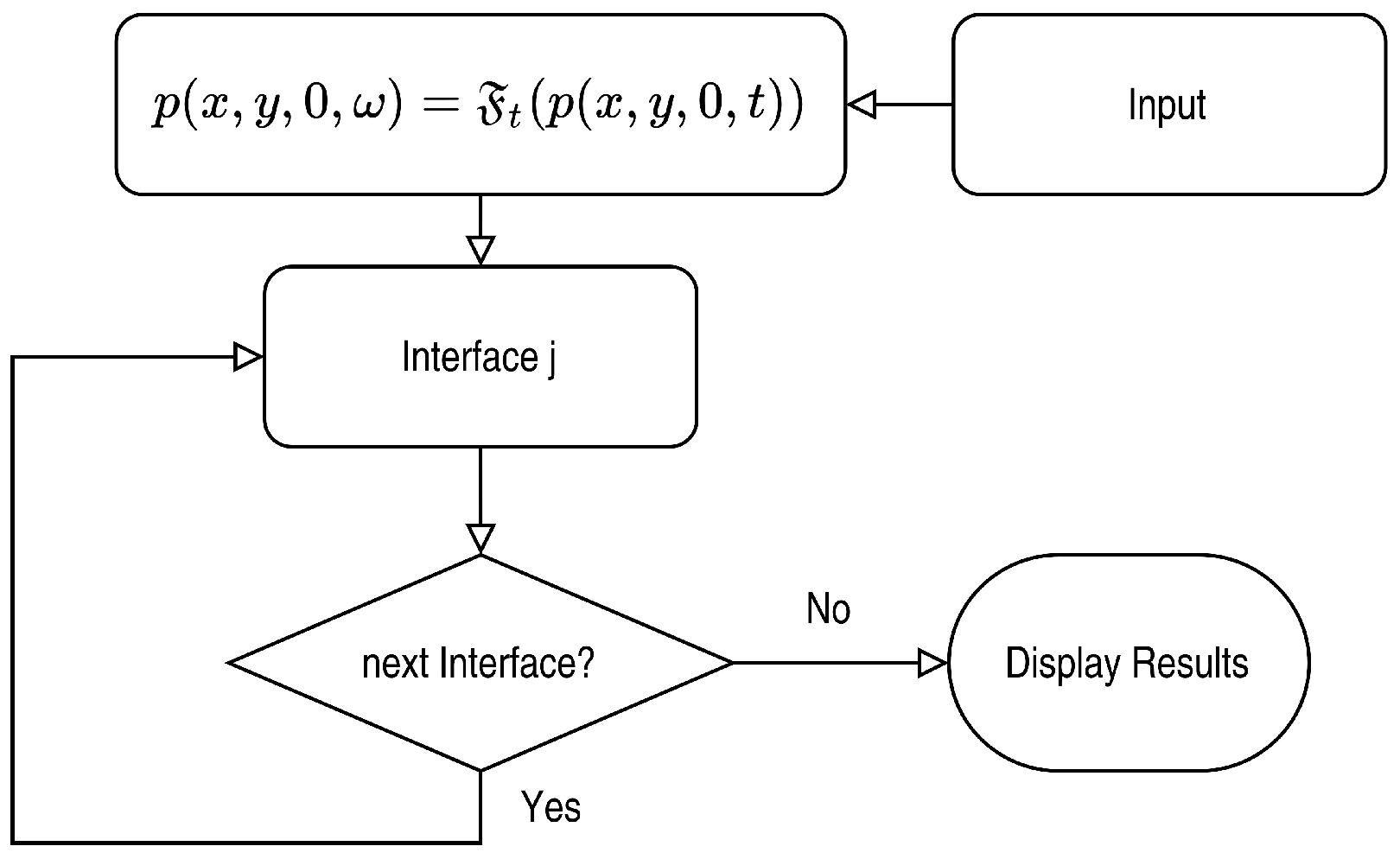
To describe the calculation from one interface to the next, the flowchart in Figure 2 is used. In the first step, the constant known parameters such as the speed of sound, density, the z-position of the interfaces, and the measured sound pressure must be set.
Then, the sound pressure is transformed in the frequency domain. The sound field generated by the incident wave at the first interface layer is determined by Equation (9) (spec-radiation method). In the block “Interface j” (with the interface number j = 1, 2, 3,...), the reflected and transmitted part is calculated. A flowchart of the block “Interface j” is depicted in Figure 3.
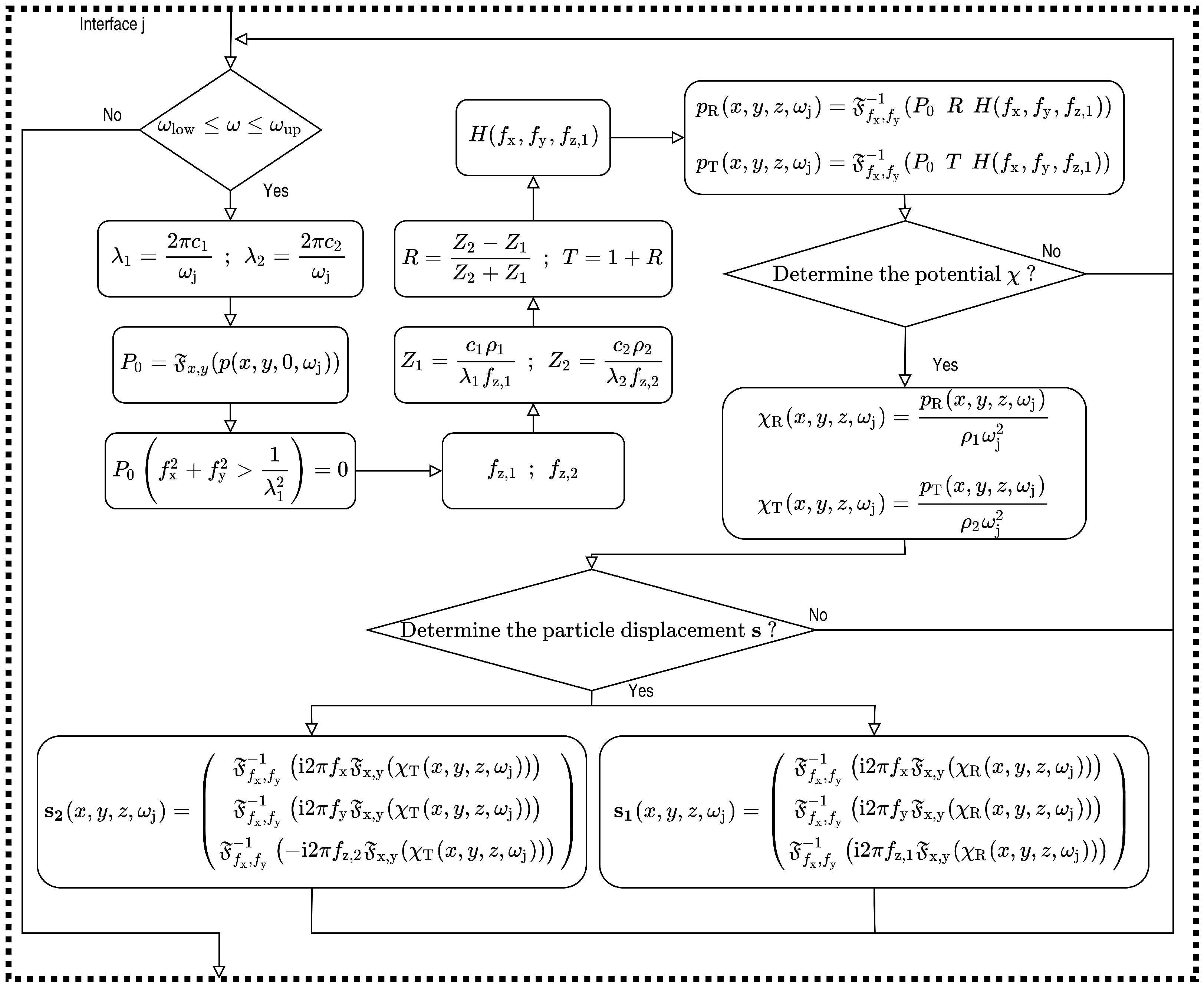
In the block “Interface j”, the first decision is among which frequencies the calculation has to be performed. For the representation of a harmonic signal, the calculation of a single frequency can be sufficient, while for the calculation of a single sinusoidal wave, several frequencies are needed. Here, all frequencies from 1.2 kHz up to 120 kHz were used. This means that 164 frequency step points were taken into account with the conjugate complex parts as well. All other frequencies were set to 0. This procedure saves much computing time. Then, the different wavelengths have to be calculated. Next, the sound pressure was transformed with a 2D FFT over the spatial coordinates. Any value that was not on the Ewald sphere was set to 0. Then, the two different spatial frequencies for the two media at the interface in the propagation direction had to be calculated. In the next step, the specific impedances and, with the specific impedances, the reflection and transmission coefficient were determined in the Fourier domain. The propagation function H was then calculated with the spatial frequency for the medium from the incident wave. In the following step, the sound pressure of the reflected and transmitted part at the interface can be calculated. If one is only interested in the sound pressure values, then the block “Interface j” could be left out. Here also, the deflection potential can be calculated, if needed, for the reflected and transmitted part. At last, in the block, the question is: Is one interested in the particle deflection? If so, then the particle deflection could be calculated from the deflection potentials in the Fourier domain as in Equation (22). Now, the block can be left alone. It has to be decided whether another interface should be determined or not. If not, then the generated results can be displayed. If so, then the block “Interface j” must be executed again. The transmitted wave up to the second interface results from the transmitted part at the first interface at . The calculation has to be considered, now that the transmitted and reflected part starts again at a local . The incident wave at Interface 2 is the transmitted part of Interface 1. As at Interface 1, the incident wave is the start for the transmitted and reflected part, and they start again at a local . After the calculation, it must be decided again whether there is another interface layer or not. It must also be decided whether the reflected sound field should be calculated back to the first interface. If this is the case, then the procedure from Figure 3 is carried out again, whereby the incident sound wave is now the reflected part of Interface 2. It was again assumed that the calculation starts at a local . For the calculation, the indices at the impedances were now simply exchanged. Similarly, for the transmission factor H, the spatial frequency of the second medium was now used, due to the fact that the incident sound wave comes from the second medium. Depending on how many reflections and transmissions through different boundary layers are to be performed, this procedure must be repeated.
2.4. Experimental Setup
This experimental setup (see Figure 4) allows the measurement of a sound field emitted by an ultrasonic transducer. The original purpose is the detection of flaws in a particleboard; hence, such a board can be placed in between the sound source and the sensor. Air was used as the coupling medium between the particleboard and the receiver/transmitter. An ultrasonic transducer called AT50 from the company Airmar was used as a transmitter. It has an active diameter of 45 mm and operates at 50 kHz. The small frequency allows large distances between the particleboard and the receiver /transmitter. However, the accuracy is lower than with higher frequencies. In air the wavelength was at 50 kHz approximately mm. Thus, due to the theory for the spec-radiation method, the smallest detectable size in air was mm. An amplitude of 100 V operates the transmitter to send out a burst of 10 sinusoidal periods with a repeating frequency of 1 Hz. With a distance of 280 mm from the transmitter to the particleboard, the distance was always larger than the near-field length (approximately 72 mm according to Krautkrämer and Krautkrämer [7]) of the transmitter in air at this frequency. The transmitter was stationary during the whole measurement. As a sample, a commercially available wooden medium-density fiberboard (MDF) was used.
The particleboard had a thickness of 25 mm. To determine the longitudinal speed of sound in the particleboard, a contact through transmission test was carried out with 50 kHz and was determined to be 450 m/s. The density of the particleboard was 730 kg/m3. As flaw imitations, pieces of paper were used (Schmelt et al. [32], Schmelt et al. [33], Schmelt and Twiefel [35], Schmelt and Twiefel [47], Marhenke et al. [30], Marhenke et al. [28]) due to the similar material properties compared to wooden particleboard. Other studies often use Teflon tape for studying CFRP or GFRP material for the same reason (Fahr [3]). When the piece of paper was placed with tape underneath the particleboard, a thin air film was always present, and this film served as the flaw imitation. It caused a similar impedance change as real air inclusion in the material. The two pieces of paper used as the flaw imitation were circular with a diameter of ø10 mm and ø6 mm, which is larger and smaller than the wavelength of 9 mm in the particleboard, but larger than the half-wavelength. The particleboard was also stationary. As a receiver, a MEMS microphone (SPU0410LR5H-QB Knowles) was used. Its upper frequency limit is 80 kHz. The receiver had a constant distance of 177 mm from the particleboard. The receiver could be moved to obtain the information for C-scans. Therefore, the XYZ-traversing stage from RoboCylinder with the traverse path of x = 0–400 mm, y = 0–200 mm, and z = 0–200 mm was used. To control the entire system, a standard computer was used. Via USB, the XYZ stage was connected to the computer and controlled by a LabView program. With a National Instruments (NI) system, the transmitter was controlled and the signal of the microphone recorded. The NI system consisted of a chassis PXIe-1085, with an inserted card for the communication with the computer (PXIe-8398), a card to record the measurement data (PXIe-5171R with a maximum sampling frequency of 250 MHz and 8 channels), and a card (PXIe-5423) as a frequency generator to control the transmitter. For the amplification of the control signal of the transmitter, the power amplifier HSA 4052 from the company NF was used to generate the required amplitude of 100 V. The measured area had a size of 152 mm × 152 mm with a measurement point distance of 2 mm in x and y. Hence, 76 × 76 points were measured, and the time step was s with a time length of s.
3. Results
3.1. Example with a Three-Layer Model
A three-layer model was selected as an example in this section. This three-layer model is shown schematically in Figure 5. The excitation was an academic piston transducer with a diameter of ø40 mm and an amplitude of one. The tilted orientation of 5 to the normal axis was computed with the procedure of Schmelt and Twiefel [47]. It emits pulse-like sinusoidal waves with a frequency of 50 kHz. The amplitude in the source plane and the time signal is displayed in Figure 6. The time step of the signal was s, and the signal was 0.000819 s long.
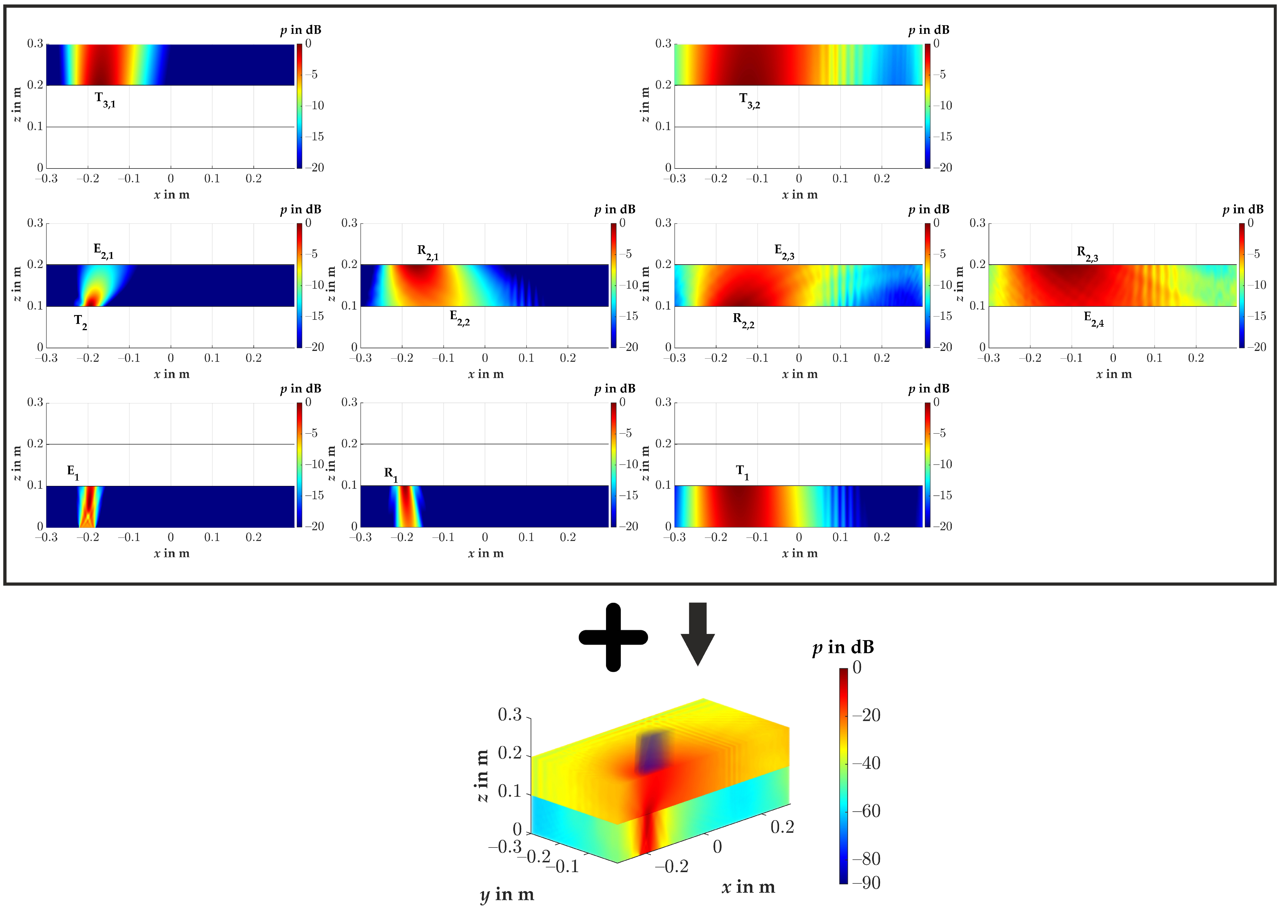
Fluids 1 and 3 were air with a speed of sound of 343 m/s and a density of 1.2041 kg/m3 Fluid 2 was water with a speed of sound of 1484 m/s and a density of 997 kg/m3. = 2 mm; ; . The simulation space had a size of 0.6 m × 0.6 m × 0.3 m (length × width × height). A step size in the z-direction of = 1 mm was used in this example. The first interface was at = 0.1 m, and the second interface was at = 0.2 m. To calculate the sound pressure between the interfaces, the spec-radiation method without the extension as in Section 2.1 can be used. Here, only the reflected and transmitted parts, as depicted in Figure 5, were calculated. More reflections and transmission can be calculated, but to demonstrate how the procedure works, only these parts were determined. The individual layers between the interfaces are shown as cross-sections in Figure 7, as well as the superpositioned result of the half-3D volume.
Here, each image was scaled in color to the maximum in the respective image to make the representation easier to understand. It can be seen that when all the results are superimposed, only with a color scaling down to −90 dB related to the maximum of the total volume, after the second interface, the transmittance becomes visible. The influences of reflection and refraction are also clearly visible. In Medium 2, it can be seen from the much wider sound field that there was a much larger wavelength present. It can be seen that from the angle of incidence of 5, an angle of approximately 22 arose in Medium 2, as defined by Snell’s law of refraction. Due to Snell’s law, the refraction angle is here:
Figure 8 depicts the particle deflection at time ms in a cross-section of the calculated volume. In Figure 8, a region between the plane m and the second interface at m is presented. It can be seen that at this time, the sound waves already reflected at the first interface. In Medium 2, the much longer wavelength, due to the higher speed of sound, was also evident. In Figure 8 is an enlarged section of the area depicted. The oscillation direction of the particles is displayed with vectors. The representation of the vectors was generated with the MATLAB function “quiver”. The vectors clearly show that the waves were longitudinal, since the direction of oscillation was in the direction of propagation.
We demonstrated with this example how the method works, that it is possible to evaluate the individual components of reflection and transmission, and that by superposition of all components, a complete sound field can be obtained. We also showed that it is possible to determine the particle deflection. We also created a video of another example of transient sound pressure propagation and included it in the Supplementary Files (Video S1). Here, using a three-layer model, as shown in Figure 3, the sound propagation can be observed. The transmitter is in the center of the volume, and only half of the volume is shown. Medium 1 is only a quarter and Medium 3 is only half as high as Medium 2. The sound pressure above in the third medium was increased by a factor of 100 because, otherwise, it would not be visible in this example. Such videos require much memory and time (some days for this example), because the time history of every point in space has to be stored and displayed.
3.2. Example with a Three-Layer Model: Perfect Impedance Match
Another academic example is the perfect impedance matching of the individual layers to each other. With a perfect impedance match, no reflections occur at an interface layer. However, this requires that the condition:
be fulfilled.
We present here the three-layer model (see Figure 5) again to demonstrate that the method presented here also included this special case. The simulation space had the same geometric dimensions as in the previous Section 3.1. The step sizes in the x-, y-, and z-directions remained as in the previous Section 3.1, and the same number of reflections and transmissions were calculated as depicted in Figure 5. The medium up to the first interface was air with a speed of sound of = 343 m/s and a density of = 1.2041 kg/m3. The second medium had a speed of sound and a density of . The third medium had a speed of sound and a density of . Thus, the conditions for the three media for perfect impedance matching were fulfilled. The same excitation signal as in Figure 6b was used, and the transmitter also had the same size and position as in Figure 6a, with the difference that the transmitter was now tilted by 10. As a result of the calculation and the superposition of all components, Figure 9 was obtained as a cross-section of the volume for the maximum sound pressure in dB related to the maximum in the entire volume.
Up to the first interface at z = 0.1 m, the tilted transmitter could be detected well. Likewise, the near-field could be identified well. A reflection from the interface was, as expected, not recognizable. After the first interface, the speed of sound in the medium was twice as high as in the first medium, which can also be recognized very well by the propagation angle. Here, as it was to be expected according to Snell’s law of refraction, it was approximately twice as large as the angle of incidence. However, no reflection can be seen even up to the second interface at z = 0.2 m, from any interface. The sound passed from Medium 2 to Medium 3 without reflection. Here, due to the fact that the speed of sound was only a quarter compared to Medium 2, the angle of propagation was also only about a quarter of what is present in Medium 2.
With this special case, we once again proved the functionality of the spec-radiation method.
3.3. Experimental Application
For the evaluation, the measured area was increased symmetrically by zero-padding to a size of 256 × 256 points with the measured area inside. With the spec-radiation method, the sound field on the board surface can be computed. The important frequency is the exciting frequency. Therefore, the evaluation was performed for a frequency of 50 kHz.
The result of this evaluation is depicted in Figure 10. In both results, the flaw may be detected, but not accurate in shape and size. This was due to the fact that the sound field behind the flaw had diffraction and interference patterns that affected the sound field on the board surface. In (a) is the result of the 10 mm flaw and in (b) the result of the 6 mm flaw. In the next step, we evaluated the result with the proposed extension, so that the result was evaluated at the z-position of the flaw in the particleboard.
We therefore calculated this through the particleboard. In contrast to the calculation of the forward propagation, it has to be considered that the start plane was the measuring plane. This means that the start sound pressure was the transmitted sound pressure . To obtain the incidence sound pressure at the interface, the transmitted sound pressure has to be divided by , so that:
The result is depicted in Figure 11. In (a), the 10 mm flaw is clearly visible as a circle with a diameter of 10 mm and the pressure drops stronger than −20 dB. In (b), the flaw with a diameter of 6 mm is visible more clearly, but is still not perfect. The area is larger than a circle of 6 mm. This was due to the fact that the 6 mm circle was close to the detection limit of /2 which was, in the wooden particleboard, approximately 4.5 mm. The pressure drop was not as strong, so that some air between the tape and the particleboard around the flaw could have raised the area here. The flaw was easier to detect in comparison with the result at the top surface of the particleboard. The evaluation time took approximately 14 s per interface layer with the corresponding dataset.
By calculating many planes from the microphone plane to the flaw plane, the sound field can also be represented as a cross-section at x = 0 m. This is depicted in Figure 12 for the ø10 mm flaw. Here, two different scalings of the results were chosen. Everything above the particleboard (z = 0 m to −0.177 m) was scaled in dB related to the maximum in the air volume above the particleboard. Everything inside the particleboard (z = −0.178 m to −0.202 m) was scaled in dB with respect to the maximum inside the particleboard. This resulted in a matching color scaling of the two areas. If everything would be scaled to the maximum inside the particleboard, it would no longer be possible to display the entire sound field in a well-recognizable color, because the sound field above the board would then be at approximately −55 dB.
From this cross-sectional view, it is clear that on the surface of the particleboard (z = −0.177 m), the flaw could not be clearly detected. What could only be detected there was a minimum of the sound pressure due to the diffraction of the sound around the flaw, as can also be seen in Figure 10a. The flaw itself, however, was completely masked by the diffraction. Only by calculating into the particleboard, the flaw became recognizable by a sound pressure drop (sound shadow) at y = 0 m. Here, the shadow extended to about half the thickness of the particleboard and had its largest diameter and strongest sound pressure drop in the plane of the flaw.
In Figure 13, the cross-sectional plane at x = 0 m is shown for the measurement with the ø6 mm flaw. There, at the position of approximately y = 0.01 m and z = −0.202 m to −0.187 m, the sound shadow of the ø6 mm flaw can be seen. Here, it is noticeable that the sound pressure drop was lower than for the ø10 mm flaw. In this figure, however, it is also clear that the supposed flaw on the surface of the particleboard in Figure 10b is deceptive. This is because the position of the flaw in the -plane could not be correctly determined with the evaluation only up to the upper surface of the particleboard, which means that an evaluation through the particleboard was necessary here.
In Figure 12 and Figure 13, there are lines to be seen, which one might think do not actually belong there. We highlighted these by way of example in Figure 13 with three arrows. These were artifacts caused by the calculation due to reflections in the measurement. Because of the narrow space and the long recording time of the measurement data, sound waves could reach the XYZ-traversing unit and were reflected from there, thus reaching the measurement area of the microphone again. In this example shown here, however, the influence on the identification of the flaws was negligible. However, such phenomena must always be taken into account in experiments of this kind.
4. Discussion
A new innovative extension for the spec-radiation method was introduced in this publication. With the spec-radiation method, we showed in the past that the detection of flaws in wooden particleboard could be performed very fast and reliably. We showed that the spec-radiation method is faster than comparable methods to detect flaws by calculating back to the top surface of a panel material (Schmelt and Twiefel [35]). We also showed that it is possible to calculate directly to the top of a tilted panel material (Schmelt and Twiefel [47]). Nevertheless, in thicker material, it is not enough to calculate the sound distribution on the top of the panel material; due to interferences and diffraction, flaws may be masked. Therefore, the next logical step was to calculate through the material. With this extension, it was now possible to calculate through different layered fluid media with the spec-radiation method. A computer with the operating system Windows 10 Pro for Workstations and 128 GB RAM and 24 cores of the type Intel(R) Xeon(R) Silver 4116 CPU @ 2.1 GHz was used for the evaluations made here. We showed on different examples how the spec-radiation method can be used to simulate and visualize sound propagation. While the representation of the maximum sound pressure in a three-dimensional volume is no longer a big challenge, the creation of three-dimensional videos is a challenge for today’s systems. For the creation of such videos, the transient information of each calculated point in space must be stored. Subsequently, all information must be called up and displayed at one point in time in order to save a frame of the video. For the three-layer model shown in Figure 7, this would be with (time × length × width × height) 4096 × 300 × 300 = 110,592,000,000 data points. With that said, there are still many possibilities for optimization since not every data point is needed for the visualization. For the detection of flaws, we showed that we can identify flaws smaller than the wavelength also in the particleboard. Here, however, it becomes clear once again that reflections from the environment must always be taken into account, as they can possibly have a negative influence on the detection of flaws.
5. Conclusions
In conclusion, with this publication, we developed a new innovative extension to the spec-radiation method. In Section 2, we described in detail both the analytical description and the practical implementation and presented an experimental setup. We showed how to calculate the particle deflection potential and the particle deflection with the spec-radiation method in the Fourier domain. We presented a flowchart model that was used to explain the practical implementation. In Section 3.1, we first showed on a three-layer model how the extension of the spec-radiation method presented here can be applied to simulate the sound propagation from a transmitter. We showed that the particle deflection can also be represented by vectors and that each reflection or transmission can be considered individually. By superposing the reflections and transmissions, we showed how the complete sound field of a 3D volume can be obtained. With a video, we showed that with this extension, it is also possible to represent the transient three-dimensional sound pressure field. With the special case of perfect impedance matching, we proved the results of the method in Section 3.2. In Section 3.3, we showed with an experiment a wooden particleboard and flaw imitations at the transmitter side that the procedure to detect flaws with the extended version of the spec-radiation method is possible. We showed that the flaws were better detectable and characterized in geometry and location by calculating the sound field through the particleboard in comparison with the result at the top surface of the particleboard. Therefore, we made the assumption that the particleboard behaves as a fluid and that only longitudinal waves propagate. We presented the result and explained the backward propagation through an interface layer. We are confident that this type of evaluation will help optimize production and quality assurance processes due to the accurate knowledge that can be gained from the flaws. Due to the very fast evaluation time, the method has great potential.
Supplementary Materials
The following are available online at https://www.mdpi.com/article/10.3390/app12031098/s1, Video S1: Transient sound propagation evaluated with the spec-radiation method.
Author Contributions
Conceptualization, A.S.S. and J.T.; methodology, A.S.S.; software, A.S.S.; validation, A.S.S. and J.T.; formal analysis, A.S.S.; investigation, A.S.S.; resources, A.S.S.; data curation, A.S.S.; writing—original draft preparation, A.S.S.; writing—review and editing, A.S.S. and J.T.; visualization, A.S.S.; supervision, J.T.; project administration, J.T.; funding acquisition, J.T. All authors have read and agreed to the published version of the manuscript.
Funding
The publication of this article was funded by the Open Access Fund of Leibniz Universität Hannover.
Institutional Review Board Statement
Not applicable.
Informed Consent Statement
Not applicable.
Acknowledgments
This research was supported by J. Wallaschek.
Conflicts of Interest
The authors declare no conflict of interest.
Abbreviations
The following abbreviations are used in this manuscript:
| CFRP | carbon-fiber-reinforced plastic |
| GFRP | glass-fiber-reinforced plastic |
| FFT | Fourier transformation |
| iFFT | inverse Fourier transformation |
| MDF | medium-density fiberboard |
| MEMS | micro-electro-mechanical systems |
References
- Jasiuniene, E.; Raisutis, R.; Sliteris, R.; Voleiis, A.; Jakas, M. Ultrasonic NDT of wind turbine blades using contact pulse-echo immersion testing with moving water container. Ultragarsas J. 2008, 63, 28–32. [Google Scholar]
- Conta, S.; Santoni, A.; Homb, A. Benchmarking the vibration velocity-based measurement methods to determine the radiated sound power from floor elements under impact excitation. Appl. Acoust. 2020, 169, 107457. [Google Scholar] [CrossRef]
- Fahr, A. Aeronautical Applications of Non-Destructive Testing; DEStech Publications, Inc.: Lancaster, PA, USA, 2014. [Google Scholar]
- Fang, Y.; Lin, L.; Feng, H.; Lu, Z.; Emms, G.W. Review of the use of air-coupled ultrasonic technologies for nondestructive testing of wood and wood products. Comput. Electron. Agric. 2017, 137, 79–87. [Google Scholar] [CrossRef]
- Sokolov, S.Y. On the problem of the propagation of ultrasonic oscillations in various bodies. Elek. Nachr. Tech. 1929, 6, 454–460. [Google Scholar]
- Deutsch, V.; Platte, M.; Vogt, M. Ultraschallprüfungen; Springer: Berlin/Heidelberg, Germany, 1997. [Google Scholar] [CrossRef]
- Krautkrämer, J.; Krautkrämer, H. Werkstoffprüfung mit Ultraschall; Springer: Berlin/Heidelberg, Germany, 1980. [Google Scholar] [CrossRef]
- Gyekenyesi, A.L.; Harmon, L.M.; Kautz, H.E. The Effect of Experimental Conditions on Acousto-Ultrasonic Reproducibility. Proc. SPIE 2002, 4704, 177–186. [Google Scholar] [CrossRef]
- Willcox, M.; Downes, G. A Brief Description of NDT Techniques; NDT Equipment Limited: Toronto, ON, Canada, 2003. [Google Scholar]
- Schafer, M. The Effect of Experimental Conditions on Acousto-Ultrasonic Reproducibility. In Proceedings of the IEEE Ultrasonics Symposium—An International Symposium (Cat. No.00CH37121), San Juan, PR, USA, 22–25 October 2000; pp. 771–778. [Google Scholar] [CrossRef]
- Green, R.E. Non-contact ultrasonic techniques. Ultrasonics 2004, 42, 9–16. [Google Scholar] [CrossRef] [PubMed]
- Zhang, Y.; Sidibé, Y.; Maze, G.; Leon, F.; Druaux, F.; Lefebvre, D. Detection of damages in underwater metal plate using acoustic inverse scattering and image processing methods. Appl. Acoust. 2016, 103, 110–121. [Google Scholar] [CrossRef]
- Mitri, F.G.; Greenleaf, J.F.; Fatemi, M. Comparison of continuous-wave (CW) and tone-burst (TB) excitation modes in vibro-acoustography: Application for the non-destructive imaging of flaws. Appl. Acoust. 2009, 70, 333–336. [Google Scholar] [CrossRef]
- Stößel, R. Air-Coupled Ultrasound Inspection as a New Non-Destructive Testing Tool for Quality Assurance. Ph.D. Thesis, Fakultät für Maschinenbau, Universität Stuttgart, Stuttgart, Germany, 2004. [Google Scholar] [CrossRef]
- Chimenti, D.E. Review of air-coupled ultrasonic materials characterization. Ultrasonics 2014, 54, 1804–1816. [Google Scholar] [CrossRef]
- Álvarez Arenas, T.E.G. Acoustic Impedance Matching of Piezoelectric Transducers to the Air. IEEE Trans. Ultrason. Ferroelectr. Freq. Control 2014, 51, 624–633. [Google Scholar] [CrossRef]
- Hillger, W.; Bühling, L.; Ilse, D. Review of 30 years ultrasonic systems and developments for the future. In Proceedings of the 11th European Conference on Non-Destructive Testing (ECNDT2014), Prague, Czech Republic, 6–10 October 2014. [Google Scholar]
- Raisutis, R.; Jasiuniene, E.; Sliteris, R.; Vladisauskas, A. The review of non-destructive testing techniques suitable for inspection of the wind turbine blades. Ultragarsas 2008, 63, 26–30. [Google Scholar]
- Sanabria, S.; Mueller, C.; Neuenschwander, J.; Niemz, P.; Sennhauser, U. Air-coupled ultrasound as an accurate and reproducible method for bonding assessment of glued timber. Wood Sci. Technol. 2011, 45, 645–659. [Google Scholar] [CrossRef] [Green Version]
- Dunky, D.; Niemz, P. Holzwerkstoffe und Leime; Springer: Berlin/Heidelberg, Germany, 2002. [Google Scholar] [CrossRef]
- Niemz, P. Bestimmung von Fehlverklebungen mittels Schallaufzeitmessung. Holz als Roh-und Werkst. 1995, 53, 236. [Google Scholar] [CrossRef]
- Bucur, V.; Böhnke, I. Factors affecting ultrasonic measurements in solid wood. Ultrasonics 1994, 32, 385–390. [Google Scholar] [CrossRef]
- Laybed, Y.; Huang, L. Ultrasound time-reversal MUSIC imaging with diffraction and attenuation compensation. IEEE Trans. Ultrason. Ferroelectr. Freq. Control 2012, 59, 2186–2200. [Google Scholar] [CrossRef]
- Döring, D. Air-Coupled Ultrasound and Guided Acoustic Waves for Application in Non-Destructive Material Testing. Ph.D. Thesis, Fakultät Luft-und Raumfahrttechnik der Universität Stuttgart, Stuttgart, Germany, 2011. [Google Scholar] [CrossRef]
- Gabor, D. Holography. Science 1972, 177, 299–313. [Google Scholar] [CrossRef]
- Singh, V. Acoustical imaging techniques for bone studies. Appl. Acoust. 1989, 27, 119–128. [Google Scholar] [CrossRef]
- Sanabria, S.; Marhenke, T.; Furrer, R.; Neuenschwander, J. Calculation of volumetric sound field of pulsed air-coupled ultrasound transducers based on single-plane measurements. IEEE Trans. Ultrason. Ferroelectr. Freq. Control 2018, 65, 72–84. [Google Scholar] [CrossRef] [PubMed]
- Marhenke, T.; Neuenschwander, J.; Furrer, R.; Zolliker, P.; Twiefel, J.; Hasener, J.; Wallaschek, J.; Sanabria, S. Air-coupled ultrasound time reversal (ACU-TR) for subwavelength non-destructive imaging. IEEE Trans. Ultrason. Ferroelectr. Freq. Control 2020, 67, 651–663. [Google Scholar] [CrossRef] [PubMed]
- Marhenke, T.; Sanabria, S.; Chintada, B.; Furrer, R.; Neuenschwander, J.; Goksel, O. Acoustic field characterization of medical array transducers based on unfocused transmits and single-plane hydrophone measurements. Sensors 2019, 19, 863. [Google Scholar] [CrossRef] [PubMed] [Green Version]
- Marhenke, T.; Sanabria, S.; Twiefel, J.; Furrer, R.; Neuenschwander, J.; Wallaschek, J. Three dimensional sound field computation and optimization of the delamination detection based on the re-radiation. In Proceedings of the 12th European Conference on Non-Destructive Testing (ECNDT 2018), Gothenburg, Sweden, 11–15 June 2018. [Google Scholar]
- Schmelt, A.; Marhenke, T.; Twiefel, J. Identifying objects in a 2D-space utilizing a novel combination of a re-radiation based method and of a difference-image-method. In Proceedings of the 23rd International Congress on Acoustics, Aachen, Germany, 9–13 September 2019. [Google Scholar]
- Schmelt, A.; Marhenke, T.; Hasener, J.; Twiefel, J. Investigation and Enhancement of the Detectability of Flaws with a Coarse Measuring Grid and Air Coupled Ultrasound for NDT of Panel Materials Using the Re-Radiation Method. Appl. Sci. 2020, 10, 1155. [Google Scholar] [CrossRef] [Green Version]
- Schmelt, A.; Li, Z.; Marhenke, T.; Twiefel, J. Aussagefähigkeit von Fehlstellenimitaten in der ZfP. In Proceedings of the DAGA 2020—46. Jahrestagung für Akustik, Hannover, Germany, 16–19 March 2020; pp. 1133–1136. [Google Scholar]
- Tsysar, S.; Sapozhnikov, O. Ultrasonic holography of 3D objects. In Proceedings of the IEEE International Ultrasonics Symposium, Rome, Italy, 20–23 September 2009; pp. 737–740. [Google Scholar] [CrossRef]
- Schmelt, A.; Twiefel, J. The Spec-Radiation Method as a Fast Alternative to the Re-Radiation Method for the Detection of Flaws in Wooden Particleboards. Appl. Sci. 2020, 10, 6663. [Google Scholar] [CrossRef]
- Wolf, E. Three-dimensional structure determination of semi-transparent objects from holographic data. Opt. Commun. 1969, 1, 153–156. [Google Scholar] [CrossRef]
- Booker, H.G.; Clemmow, P.C. The concept of an angular spectrum of plane waves, and its relation to that of polar diagram and aperture distribution. IEEE-Part III Radio Commun. Eng. 1950, 97, 11–17. [Google Scholar] [CrossRef] [Green Version]
- Ratcliffe, J.A. Some Aspects of Diffraction Theory and their Application to the Ionosphere. Rep. Prog. Phys. 1956, 19, 188–267. [Google Scholar] [CrossRef]
- Boyer, A.L.; Hirsch, P.M.; Jordan, J.A.; Lesem, L.B.; Van Rooy, D.L. Reconstruction of tultrasonic images by backward propagation. Proc. Acoust. Hologr. 1970, 3, 333–348. [Google Scholar] [CrossRef]
- Schafer, M.E.; Lewin, P.A. Transducer characterization using the angular spectrum method. J. Acoust. Soc. Am. 1989, 85, 2202–2214. [Google Scholar] [CrossRef]
- de Belleval, J.F.; Messaoud-Nacer, N. Ultrasonic transducer beams model, using transient angular spectrum. Rev. Prog. Quant. Nondestruct. Eval. 1999, 18, 1101–1106. [Google Scholar] [CrossRef]
- Peng, H.; Lu, J.; Han, X. High frame rate ultrasonic imaging system based on the angular spectrum principle. Ultrasonics 2006, 44, e97–e99. [Google Scholar] [CrossRef]
- Yan, X.; Hamilton, M.F. Angular spectrum decomposition analysis of second harmonic ultrasound propagation and its relation to tissue harmonic imaging. In Ultrasonic and Advanced Methods for Nondestructive Testing and Material Characterization; e-Journal of Nondestructive Testing (NDT); World Scientific Publishing: Singapore, 2007; pp. 155–168. ISSN 1435-4934. [Google Scholar] [CrossRef] [Green Version]
- Aanes, M.; Lohne, K.D.; Lunde, P.; Vestrheim, M. Ultrasonic beam transmission through a water-immersed plate at oblique incidence using a piezoelectric source transducer Finite element-angular spectrum modeling and measurements. In Proceedings of the 2012 IEEE International Ultrasonics Symposium, Dresden, Germany, 7–10 October 2012; pp. 1972–1977. [Google Scholar] [CrossRef]
- Liu, D.L.; Waag, R.C. Propagation and backpropagation for ultrasonic wavefront design. IEEE Trans. Ultrason. Ferroelectr. Freq. Control 1997, 44, 1–13. [Google Scholar] [CrossRef]
- Matsushima, K. Introduction to Computer Holography; Springer: Cham, Switzerland, 2020. [Google Scholar] [CrossRef]
- Schmelt, A.; Twiefel, J. Flaw Detection on a Tilted Particleboard by Use of the Spec-Radiation Method. Appl. Sci. 2020, 10, 8513. [Google Scholar] [CrossRef]
- Goodman, J.W. Introduction to Fourier Optics; W. H. Freeman and Company: New York, NY, USA, 2017. [Google Scholar]
- Brekhovskikh, L.M.; Godin, O.A. Acoustics of Layered Media I; Springer: Heidelberg, Germany, 2020. [Google Scholar] [CrossRef]
- Möser, M. Analyse und Synthese Akustischer Spektren; Springer: Berlin/Heidelberg, Germany, 1988. [Google Scholar]
Figure 1.
Schematic representation of the incident, reflected, and transmitted waves at a fluid–fluid interface in a semi-infinite volume. Included are the speed of sound and , the densities and , and the wavelengths and of the two fluid media.
Figure 1.
Schematic representation of the incident, reflected, and transmitted waves at a fluid–fluid interface in a semi-infinite volume. Included are the speed of sound and , the densities and , and the wavelengths and of the two fluid media.

Figure 2.
Flowchart for the practical realization of the spec-radiation method for layered fluid media.
Figure 2.
Flowchart for the practical realization of the spec-radiation method for layered fluid media.

Figure 3.
Flowchart of the block ”Interface j” for the practical realization of the spec-radiation method for layered fluid media.
Figure 3.
Flowchart of the block ”Interface j” for the practical realization of the spec-radiation method for layered fluid media.

Figure 4.
Experimental setup.

Figure 5.
Schematic representation of the 3-layer fluid model. Depicted are the incident , reflected , and transmitted waves at fluid–fluid interfaces. n is the number of interfaces, and m is the number of interactions (example: is the third reflection in the fluid at Interface 2). is the height of the fluid layer; is the density; is the wavelength.

Figure 6.
(a) Sound pressure amplitude of the tilted academic piston transducer in the plane m; (b) transient pressure signal of the academic piston transducer.
Figure 6.
(a) Sound pressure amplitude of the tilted academic piston transducer in the plane m; (b) transient pressure signal of the academic piston transducer.

Figure 7.
Calculated sound fields in the layered fluids and the superposition of the sound fields.

Figure 8.
Particle deflection in a cross-section of the calculated volume of Figure 7 at time 0.4 ms with an enlarged section to show with vectors that here, there are longitudinal waves propagating.
Figure 8.
Particle deflection in a cross-section of the calculated volume of Figure 7 at time 0.4 ms with an enlarged section to show with vectors that here, there are longitudinal waves propagating.

Figure 9.
Maximum sound pressure in dB related to the maximum in the entire volume. Perfect impedance matching of a 3-layer model. The results were evaluated for frequencies up to 250 MHz.
Figure 9.
Maximum sound pressure in dB related to the maximum in the entire volume. Perfect impedance matching of a 3-layer model. The results were evaluated for frequencies up to 250 MHz.

Figure 10.
Evaluation result on the top surface of the wooden particleboard, with (a) 10 mm and (b) 6 mm under the particleboard. The results were evaluated at a frequency of 50 kHz.
Figure 10.
Evaluation result on the top surface of the wooden particleboard, with (a) 10 mm and (b) 6 mm under the particleboard. The results were evaluated at a frequency of 50 kHz.

Figure 11.
Evaluation result on the lower surface of the wooden particleboard, with (a) 10 mm and (b) 6 mm under the particleboard. The results were evaluated at a frequency of 50 kHz.
Figure 11.
Evaluation result on the lower surface of the wooden particleboard, with (a) 10 mm and (b) 6 mm under the particleboard. The results were evaluated at a frequency of 50 kHz.

Figure 12.
Cross-section plane at x = 0 m of the calculated volume with the ø10 mm flaw. The sound pressure is shown in dB. For the color scaling in the air, the maximum of the sound pressure in the air volume is taken up to the surface of the particleboard (z = 0 m to −0.177 m). For the color scaling in the particleboard, the maximum sound pressure in the particleboard (z = −0.178 m to −0.202 m) is used. If both are now displayed up to −20 dB, the result is a matching color scale. The results were evaluated at a frequency of 50 kHz.

Figure 13.
Cross-section plane at x = 0 m of the calculated volume with the ø6 mm flaw. The sound pressure is shown in dB. For the color scaling in the air, the maximum of the sound pressure in the air volume is taken up to the surface of the particleboard (z = 0 m to −0.177 m). For the color scaling in the particleboard, the maximum sound pressure in the particleboard (z = −0.178 m to −0.202 m) is used. If both are now displayed up to −20 dB, the result is a matching color scale. The results were evaluated at a frequency of 50 kHz.

Publisher’s Note: MDPI stays neutral with regard to jurisdictional claims in published maps and institutional affiliations. |
© 2022 by the authors. Licensee MDPI, Basel, Switzerland. This article is an open access article distributed under the terms and conditions of the Creative Commons Attribution (CC BY) license (https://creativecommons.org/licenses/by/4.0/).
Share and Cite
MDPI and ACS Style
Schmelt, A.S.; Twiefel, J. The Spec-Radiation Method for Layered Fluid Media. Appl. Sci. 2022, 12, 1098. https://doi.org/10.3390/app12031098
AMA Style
Schmelt AS, Twiefel J. The Spec-Radiation Method for Layered Fluid Media. Applied Sciences. 2022; 12(3):1098. https://doi.org/10.3390/app12031098
Chicago/Turabian StyleSchmelt, Andreas Sebastian, and Jens Twiefel. 2022. "The Spec-Radiation Method for Layered Fluid Media" Applied Sciences 12, no. 3: 1098. https://doi.org/10.3390/app12031098
Note that from the first issue of 2016, this journal uses article numbers instead of page numbers. See further details here.