
Research and Verification of Trajectory Tracking Control of a Quadrotor Carrying a Load


Abstract
:1. Introduction
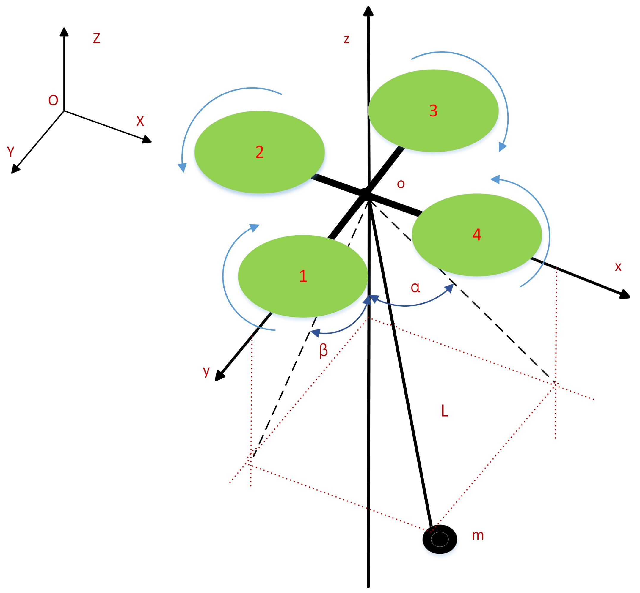
2. Establishment of a Quadrotor Carrying a Load
- The weight and moment of inertia of the quadrotor remain constant.
- The hanging rope is rigid and independent of the mass.
- The load always hangs from the center of the mass of the quadrotor.
- The payload is considered as a point-mass.
- The hanging load always hangs below the quadrotor, i.e., the swing angle of a quadrotor carrying a load is always between .
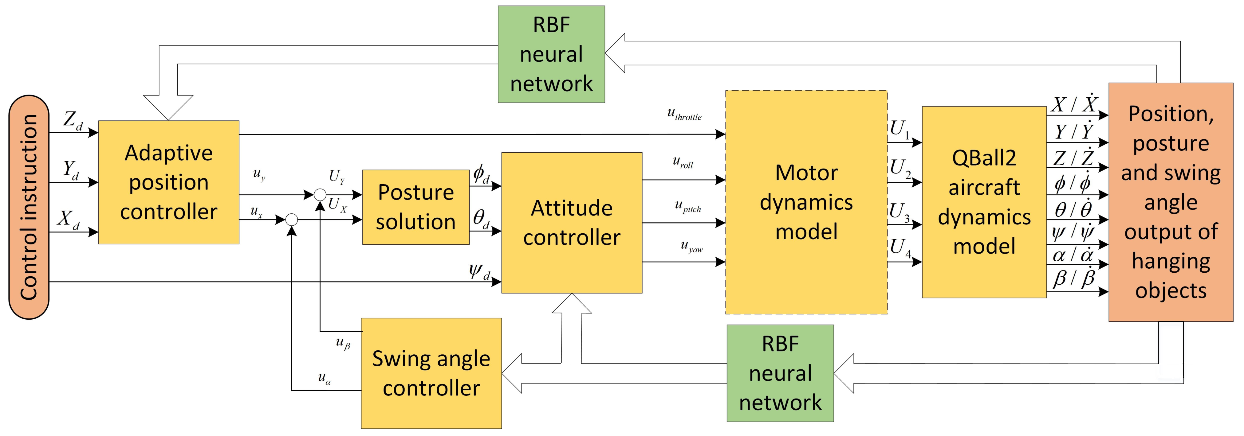
3. Controller Design
3.1. Attitude Controller Design
3.2. Stability Analysis
3.3. Position Controller Design
3.4. Swing Angle Controller Design
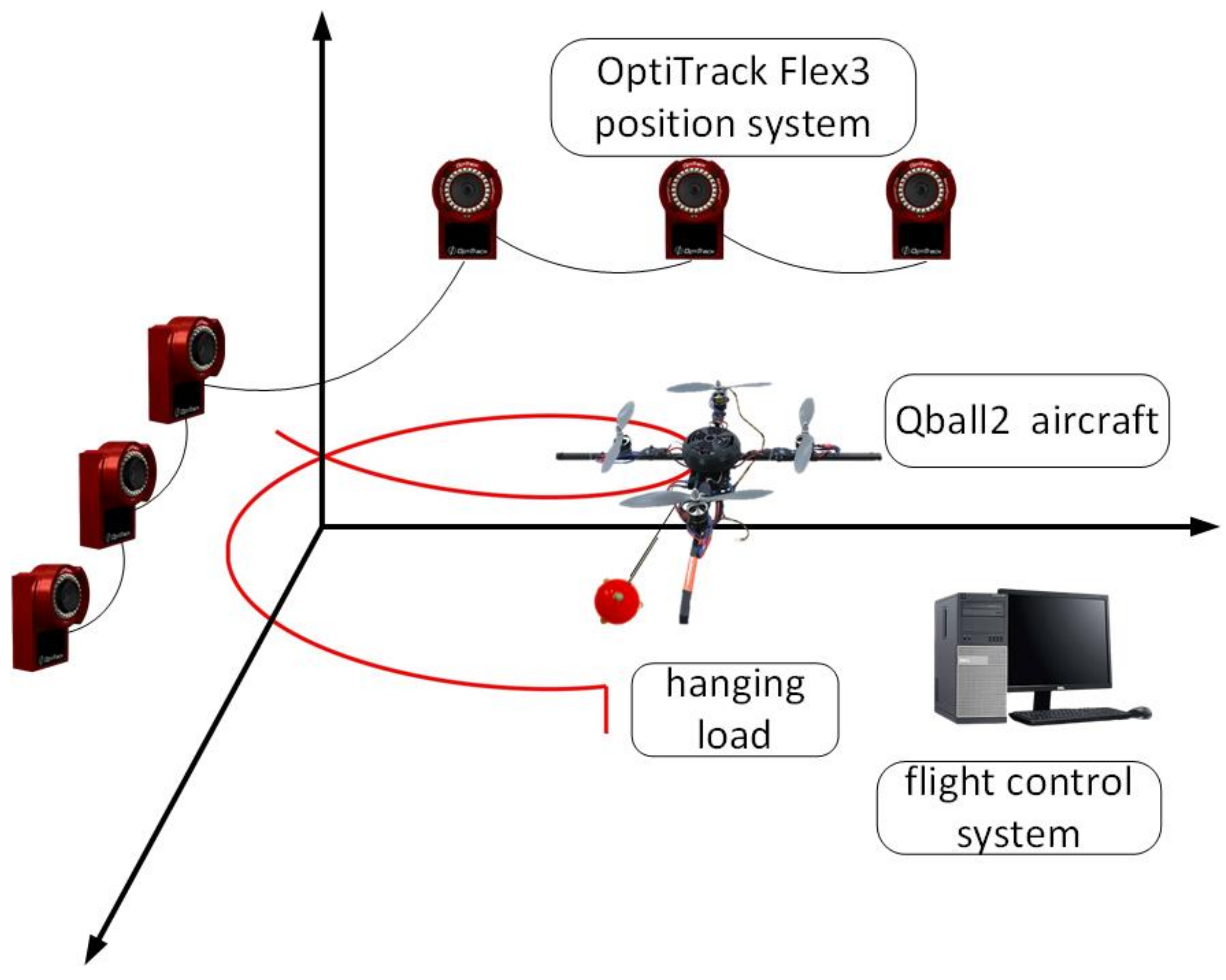
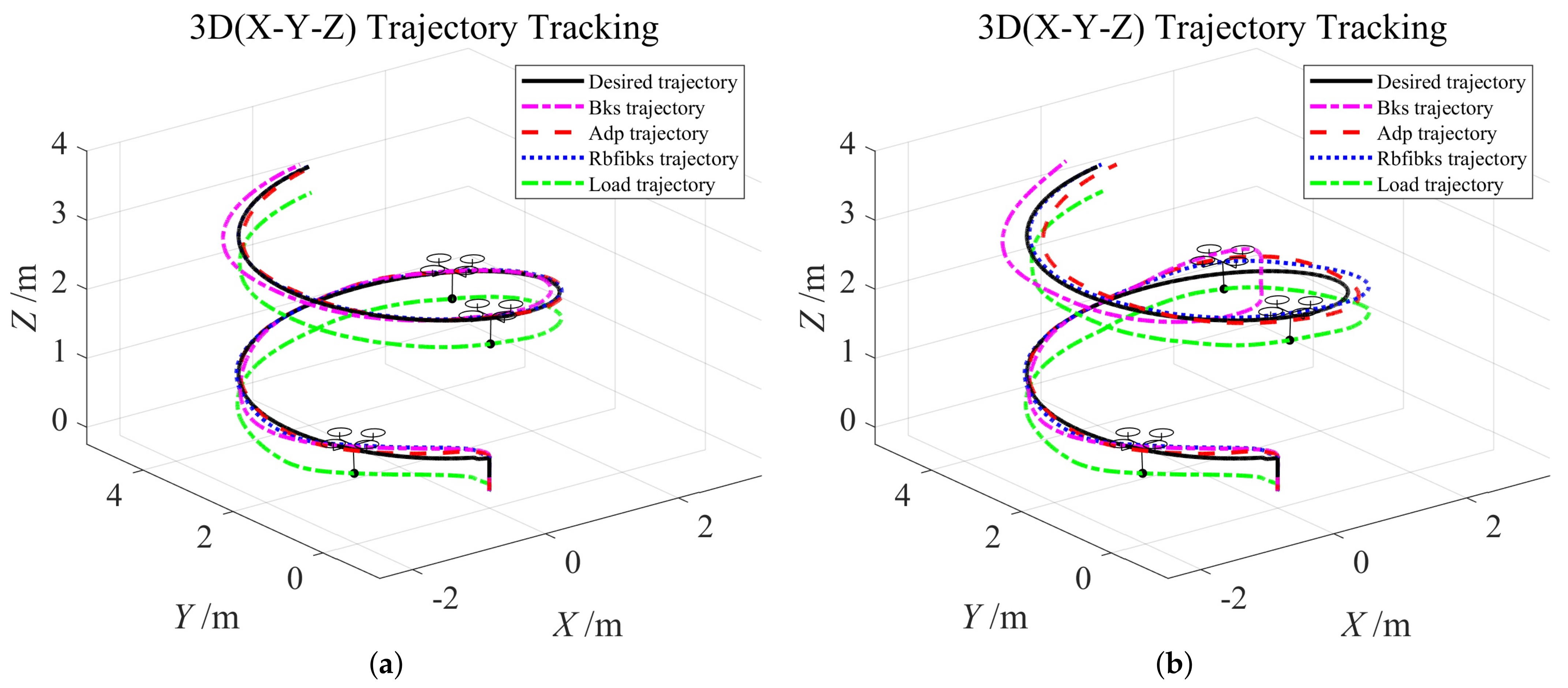
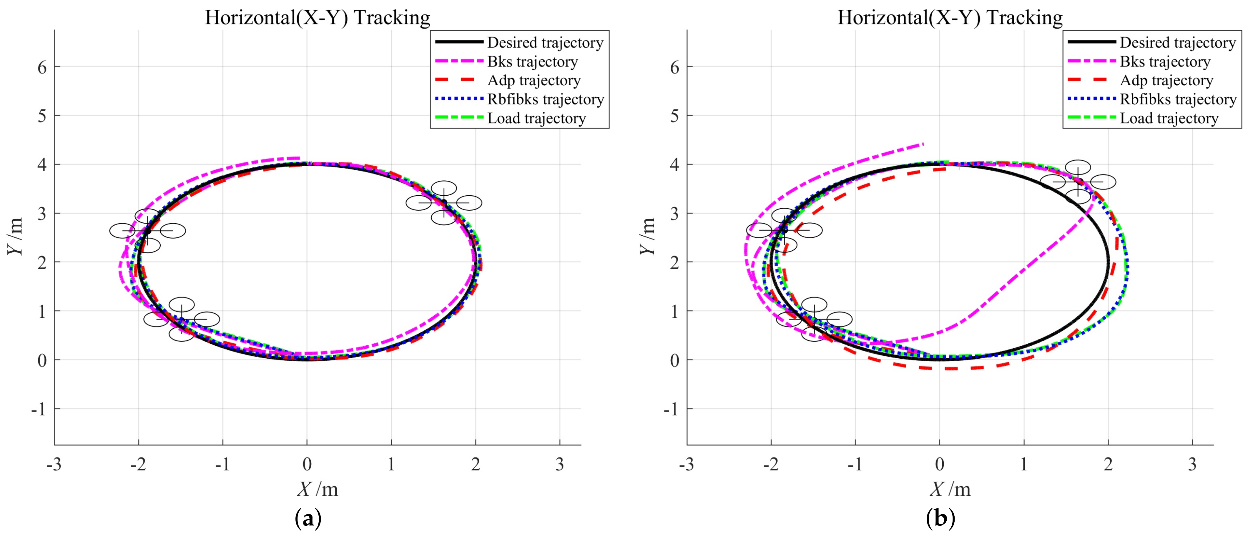
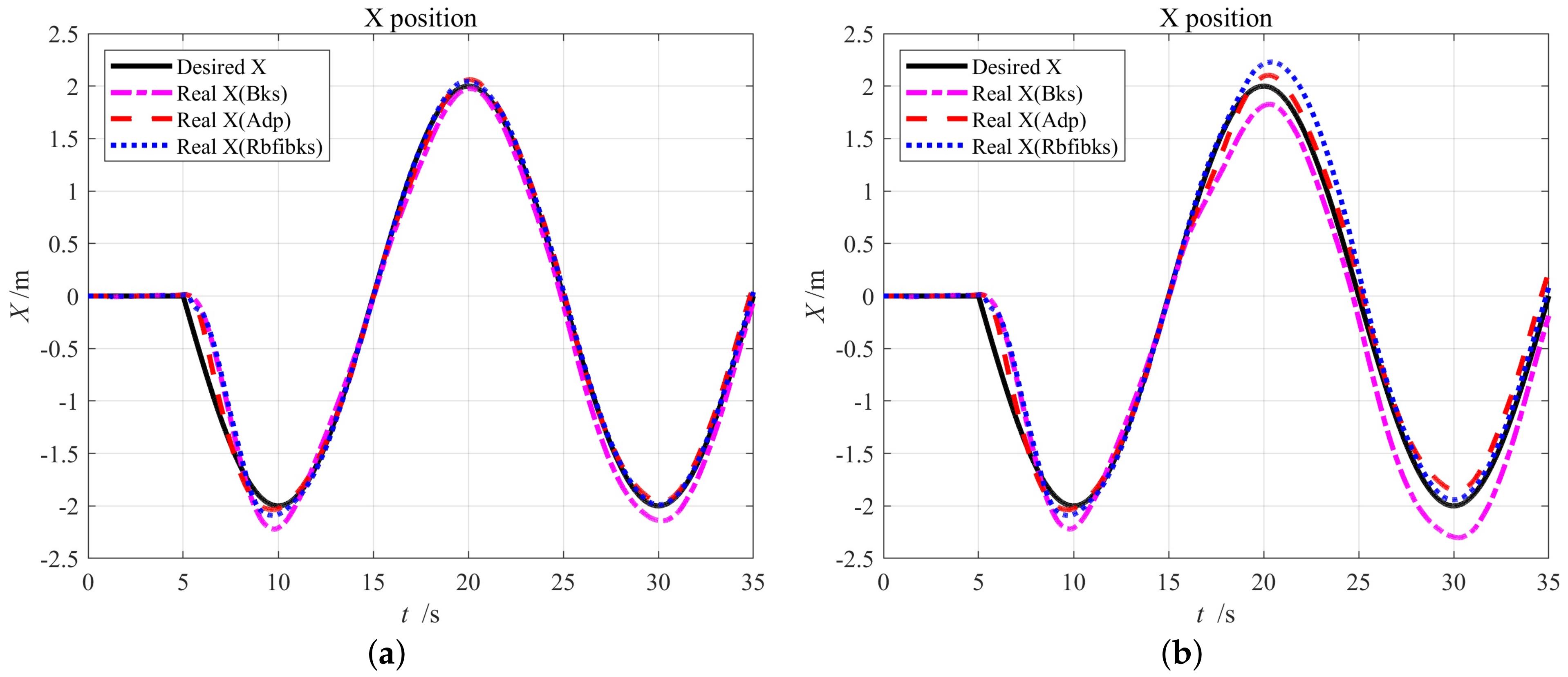
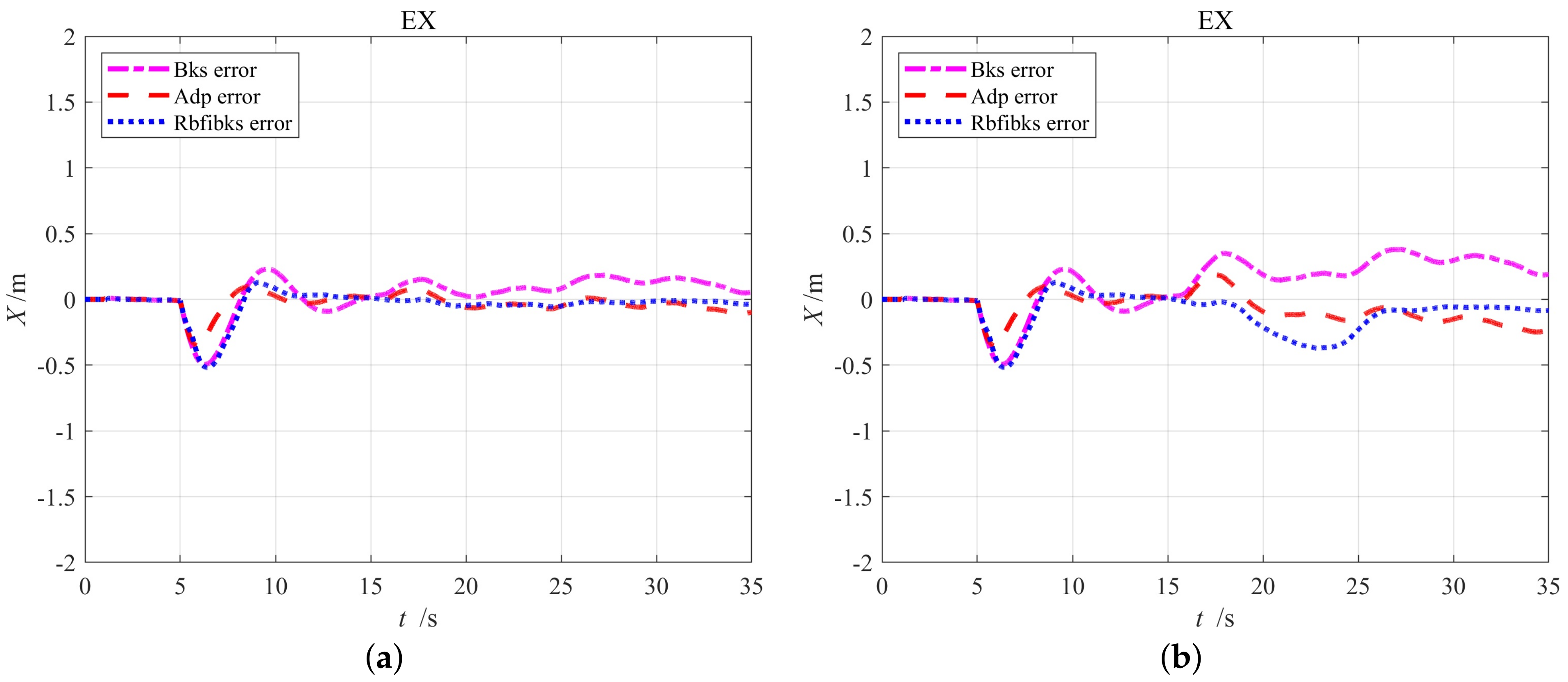
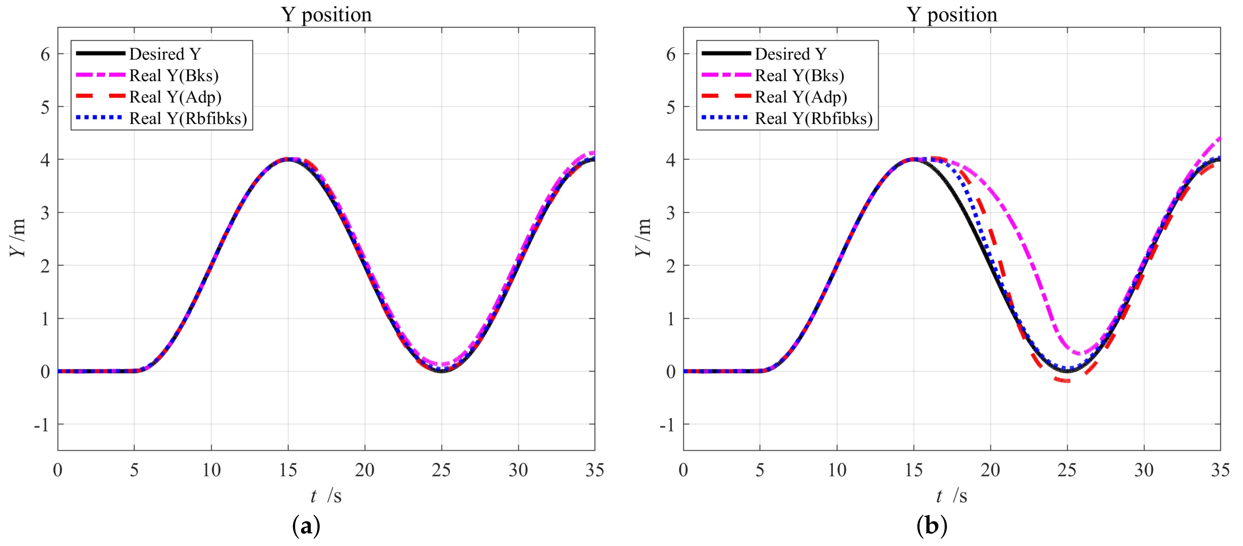
4. Simulation Verification
5. Conclusions
Author Contributions
Funding
Institutional Review Board Statement
Informed Consent Statement
Data Availability Statement
Conflicts of Interest
References
- Sreenath, K.; Lee, T.; Kumar, V. Geometric control and differential flatness of a quadrotor UAV with a cable-suspended load. In Proceedings of the 52nd IEEE Conference on Decision and Control, Firenze, Italy, 10–13 December 2013; pp. 2269–2274. [Google Scholar] [CrossRef]
- Jackson, B.E.; Howell, T.A.; Shah, K.; Schwager, M.; Manchester, Z. Scalable Cooperative Transport of Cable-Suspended Loads With UAVs Using Distributed Trajectory Optimization. IEEE Robot. Autom. Lett. 2020, 5, 3368–3374. [Google Scholar] [CrossRef]
- Sanalitro, D.; Savino, H.J.; Tognon, M.; Cortés, J.; Franchi, A. Full-Pose Manipulation Control of a Cable-Suspended Load With Multiple UAVs Under Uncertainties. IEEE Robot. Autom. Lett. 2020, 5, 2185–2191. [Google Scholar] [CrossRef] [Green Version]
- Dai, S.; Lee, T.; Bernstein, D.S. Adaptive control of a quadrotor UAV transporting a cable-suspended load with unknown mass. In Proceedings of the 53rd IEEE Conference on Decision and Control, Los Angeles, CA, USA, 15–17 December 2014; pp. 6149–6154. [Google Scholar] [CrossRef]
- Alothman, Y.; Jasim, W.; Gu, D. Quad-rotor lifting-transporting cable-suspended payloads control. In Proceedings of the 2015 21st International Conference on Automation and Computing (ICAC), Glasgow, UK, 11–12 September 2015; pp. 1–6. [Google Scholar] [CrossRef]
- Alothman, Y.; Gu, D. Quadrotor transporting cable-suspended load using iterative Linear Quadratic regulator (iLQR) optimal control. In Proceedings of the 2016 8th Computer Science and Electronic Engineering (CEEC), Colchester, UK, 28–30 September 2016; pp. 168–173. [Google Scholar] [CrossRef]
- Guerrero, M.E.; Mercado, D.A.; Lozano, R.; García, C.D. Passivity based control for a quadrotor UAV transporting a cable-suspended payload with minimum swing. In Proceedings of the 2015 54th IEEE Conference on Decision and Control (CDC), Osaka, Japan, 15–18 December 2015; pp. 6718–6723. [Google Scholar] [CrossRef]
- Zeng, J.; Kotaru, P.; Sreenath, K. Geometric Control and Differential Flatness of a Quadrotor UAV with Load Suspended from a Pulley. In Proceedings of the 2019 American Control Conference (ACC), Philadelphia, PA, USA, 10–12 July 2019; pp. 2420–2427. [Google Scholar] [CrossRef]
- Yang, S.; Xian, B. Exponential Regulation Control of a Quadrotor Unmanned Aerial Vehicle With a Suspended Payload. IEEE Trans. Control Syst. Technol. 2020, 28, 2762–2769. [Google Scholar] [CrossRef]
- Su, J.; Bak, J.; Hyun, J. Optimal Trajectory Generation for Quadrotor with Suspended Load Under Swing Angle Constraint. In Proceedings of the 2019 IEEE 15th International Conference on Control and Automation (ICCA), Edinburgh, UK, 16–19 July 2020; pp. 549–554. [Google Scholar] [CrossRef]
- Tang, S.; Kumar, V. Mixed Integer Quadratic Program trajectory generation for a quadrotor with a cable-suspended payload. In Proceedings of the 2015 IEEE International Conference on Robotics and Automation (ICRA), Seattle, WA, USA, 26–30 May 2015; pp. 2216–2222. [Google Scholar] [CrossRef]
- Chen, X.; Zhao, Y.; Fan, Y. Adaptive Integral Backstepping Control for a Quadrotor with Suspended Flight. In Proceedings of the 2020 5th International Conference on Automation, Control and Robotics Engineering (CACRE), Dalian, China, 19–20 September 2020; pp. 226–234. [Google Scholar] [CrossRef]
- Pizetta, I.H.; Brandão, A.S.; Sarcinelli-Filho, M. Modelling and control of a PVTOL quadrotor carrying a suspended load. In Proceedings of the 2015 International Conference on Unmanned Aircraft Systems (ICUAS), Denver, CO, USA, 9–12 June 2015; pp. 444–450. [Google Scholar] [CrossRef]
- Qian, L.; Liu, H.H. Dynamics and control of a quadrotor with a cable suspended payload. In Proceedings of the 2017 IEEE 30th Canadian Conference on Electrical and Computer Engineering (CCECE), Windsor, ON, Canada, 30 April–3 May 2017; pp. 1–4. [Google Scholar] [CrossRef]
- Tang, S.; Wüest, V.; Kumar, V. Aggressive Flight With Suspended Payloads Using Vision-Based Control. IEEE Robot. Autom. Lett. 2018, 3, 1152–1159. [Google Scholar] [CrossRef]
- Mo, R.; Geng, Q.; Lu, X. Study on control method of a rotor UAV transportation with slung-load. In Proceedings of the 2016 35th Chinese Control Conference (CCC), Chengdu, China, 27–29 July 2016; pp. 3274–3279. [Google Scholar] [CrossRef]
- Villa, D.K.; Brandao, A.S.; Sarcinelli-Filho, M. A Survey on Load Transportation Using Multirotor UAVs. J. Intell. Robot. Syst. 2020, 98, 267–296. [Google Scholar] [CrossRef]
- Gawel, A.; Kamel, M.; Novkovic, T.; Widauer, J.; Nieto, J. Aerial picking and delivery of magnetic objects with MAVs. In Proceedings of the 2017 IEEE International Conference on Robotics and Automation (ICRA), Singapore, 29 May–3 June 2017; pp. 5746–5752. [Google Scholar] [CrossRef] [Green Version]
- Gassner, M.; Cieslewski, T.; Scaramuzza, D. Dynamic collaboration without communication: Vision-based cable-suspended load transport with two quadrotors. In Proceedings of the 2017 IEEE International Conference on Robotics and Automation (ICRA), Singapore, 29 May–3 June 2017; pp. 5196–5202. [Google Scholar] [CrossRef] [Green Version]
- Tang, S.; Wüest, V.; Kumar, V. Grasping from the air: Hovering capture and load stability. In Proceedings of the 2011 IEEE International Conference on Robotics and Automation, Shanghai, China, 9–13 May 2011; pp. 2491–2498. [Google Scholar] [CrossRef]
- Zeng, J.; Sreenath, K. Geometric Control of a Quadrotor with a Load Suspended from an Offset. In Proceedings of the 2019 American Control Conference (ACC), Philadelphia, PA, USA, 10–12 July 2019; pp. 3044–3050. [Google Scholar] [CrossRef]
- Zúñiga, N.S.; Muñoz, F.; Márquez, M.A.; Espinoza, E.S.; Carrillo, L.R. Load transportation using single and multiple quadrotor aerial vehicles with swing load attenuation. In Proceedings of the 2018 International Conference on Unmanned Aircraft Systems (ICUAS), Dallas, TX, USA, 12–15 June 2018; pp. 269–278. [Google Scholar] [CrossRef]
- Hashemi, D.; Heidari, H. Trajectory Planning of Quadrotor UAV with Maximum Payload and Minimum Oscillation of Suspended Load Using Optimal Control. J. Intell. Robatic Syst. 2020, 100, 1369–1381. [Google Scholar] [CrossRef]
- Alkomy, H.; Shan, J. Vibration reduction of a quadrotor with a cable-suspended payload using polynomial trajectories. Nonlinear Dyn. 2021, 104, 3713–3735. [Google Scholar] [CrossRef] [PubMed]
- Yu, G.; Cabecinhas, D.; Cunha, R.; Silvestre, C. Nonlinear Backstepping Control of a Quadrotor-Slung Load System. IEEE/ASME Trans. Mechatronics 2019, 24, 2304–2315. [Google Scholar] [CrossRef]
- Cabecinhas, D.; Cunha, R.; Silvestre, C. A nonlinear quadrotor trajectory tracking controller with disturbance rejection. In Proceedings of the 2014 American Control Conference, Portland, OR, USA, 4–6 June 2014; pp. 560–565. [Google Scholar] [CrossRef]
- Liang, X.; Fang, Y.; Sun, N.; Lin, H. Nonlinear Hierarchical Control for Unmanned Quadrotor Transportation Systems. IEEE Trans. Ind. Electron. 2018, 65, 3395–3405. [Google Scholar] [CrossRef]
- Allahverdy, D.; Fakharian, A.; Menhaj, M.B. Back-Stepping Integral Sliding Mode Control with Iterative Learning Control Algorithm for Quadrotor UAV Transporting Cable-Suspended Payload. In Proceedings of the 2021 29th Iranian Conference on Electrical Engineering (ICEE), Tehran, Iran, 18–20 May 2021; pp. 660–665. [Google Scholar] [CrossRef]
- Lori, A.A.; Danesh, M.; Amiri, P.; Ashkoofaraz, S.Y.; Azargoon, M.A. Transportation of an Unknown Cable-Suspended Payload by a Quadrotor in Windy Environment under Aerodynamics Effects. In Proceedings of the 2021 7th International Conference on Control, Instrumentation and Automation (ICCIA), Tabriz, Iran, 23–24 February 2021; pp. 1–6. [Google Scholar] [CrossRef]
- Yang, T.; Sun, N.; Fang, Y. Adaptive Fuzzy Control for a Class of MIMO Underactuated Systems With Plant Uncertainties and Actuator Deadzones: Design and Experiments. IEEE Trans. Cybern. 2021, 1–14. [Google Scholar] [CrossRef] [PubMed]
- Yang, T.; Sun, N.; Fang, Y. Neuroadaptive Control for Complicated Underactuated Systems With Simultaneous Output and Velocity Constraints Exerted on Both Actuated and Unactuated States. IEEE Trans. Neural Netw. Learn. Syst. 2021, 1–11. [Google Scholar] [CrossRef] [PubMed]
- Fan, Y.; Cao, Y.; Zhao, Y. Design of the nonlinear controller for a quadrotor trajectory tracking. In Proceedings of the 2017 29th Chinese Control And Decision Conference (CCDC), Chongqing, China, 28–30 May 2017; pp. 2162–2167. [Google Scholar]
- Fan, Y.; Cao, Y.; Li, T. Adaptive integral backstepping control for trajectory tracking of a quadrotor. In Proceedings of the 2017 4th International Conference on Information, Cybernetics and Computational Social Systems (ICCSS), Dalian, China, 24–26 July 2017; pp. 619–624. [Google Scholar] [CrossRef]


| Parameter | Value | Parameter | Value |
|---|---|---|---|
| M | 1.80 kg | 0.03 kg | |
| l | 0.20 m | 0.03 kg | |
| m | 0.2 kg | 0.04 kg | |
| L | 0.4 m | 8.80 N | |
| w | 15 rad/s | 0.40 N | |
| g | 9.81 m/() |
| Interference | Bks | Adp | Rbf |
|---|---|---|---|
| Weak | 0.1062 m | 0.0536 m | 0.0489 m |
| Strong | 0.1878 m | 0.1156 m | 0.0962 m |
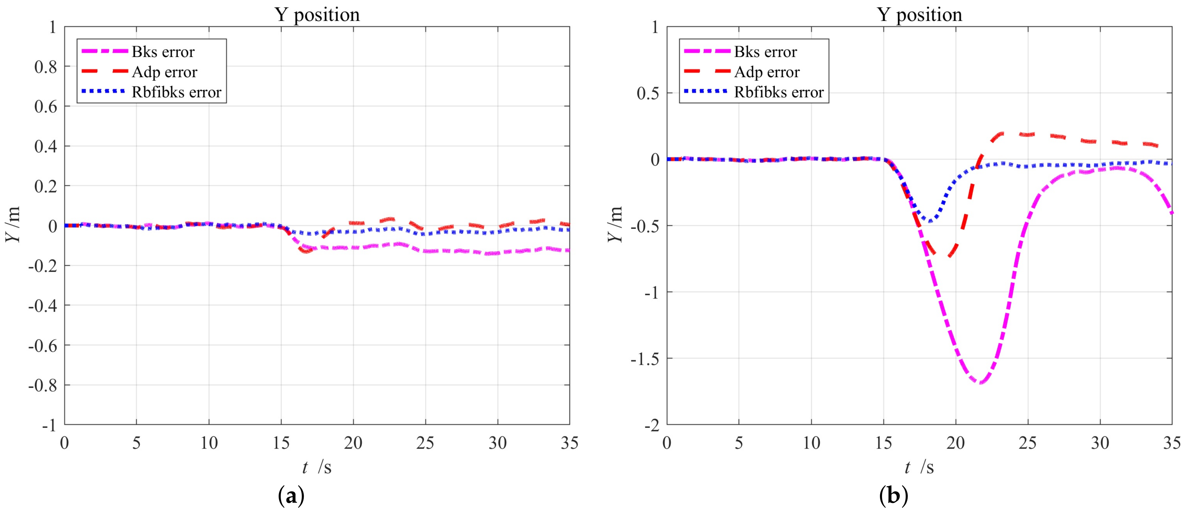
| Interference | Bks | Adp | Rbf |
|---|---|---|---|
| Weak | 0.0668 m | 0.0181 m | 0.0168 m |
| Strong | 0.3190 m | 0.1355 m | 0.0596 m |
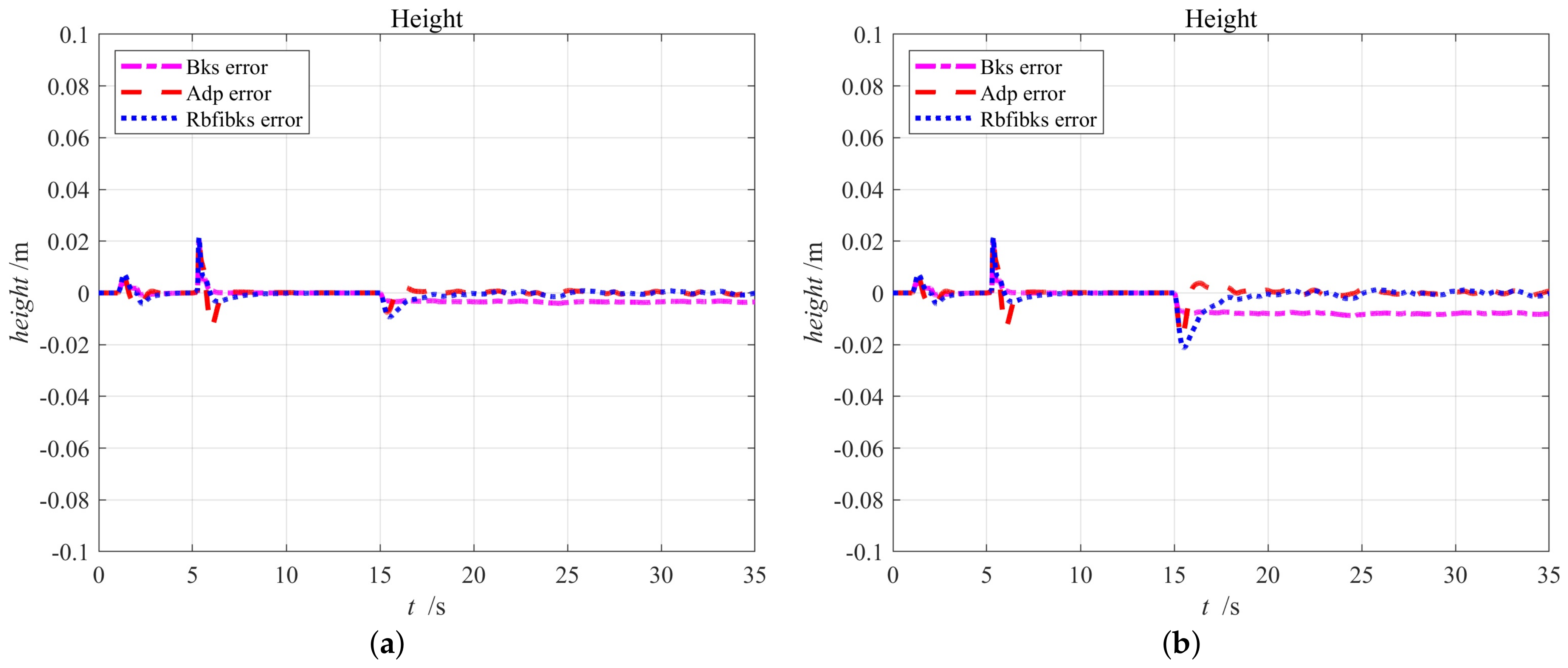
| Interference | Bks | Adp | Rbf |
|---|---|---|---|
| Weak | 0.0022 m | 0.0010 m | 0.0008 m |
| Strong | 0.0047 m | 0.0016 m | 0.0011 m |
Publisher’s Note: MDPI stays neutral with regard to jurisdictional claims in published maps and institutional affiliations. |
© 2022 by the authors. Licensee MDPI, Basel, Switzerland. This article is an open access article distributed under the terms and conditions of the Creative Commons Attribution (CC BY) license (https://creativecommons.org/licenses/by/4.0/).
Share and Cite
Fan, Y.; Guo, H.; Han, X.; Chen, X. Research and Verification of Trajectory Tracking Control of a Quadrotor Carrying a Load. Appl. Sci. 2022, 12, 1036. https://doi.org/10.3390/app12031036
Fan Y, Guo H, Han X, Chen X. Research and Verification of Trajectory Tracking Control of a Quadrotor Carrying a Load. Applied Sciences. 2022; 12(3):1036. https://doi.org/10.3390/app12031036
Chicago/Turabian StyleFan, Yunsheng, Hongrun Guo, Xinjie Han, and Xinyu Chen. 2022. "Research and Verification of Trajectory Tracking Control of a Quadrotor Carrying a Load" Applied Sciences 12, no. 3: 1036. https://doi.org/10.3390/app12031036