
Mobility Prediction of Mobile Wireless Nodes


Abstract
:1. Introduction and Motivation
2. Mobility Models
2.1. Gauss–Markov
2.2. Random Waypoint
2.3. Random Walk
2.4. Random Direction
2.5. RSSGM
3. Machine Learning Classifiers
3.1. Logistic Regression
3.2. Decision Tree
3.3. K-Nearest Neighbors
3.4. Latent Dirichlet Allocation
3.5. Gaussian Naive Bayes
3.6. Support Vector Machines
4. Related Works
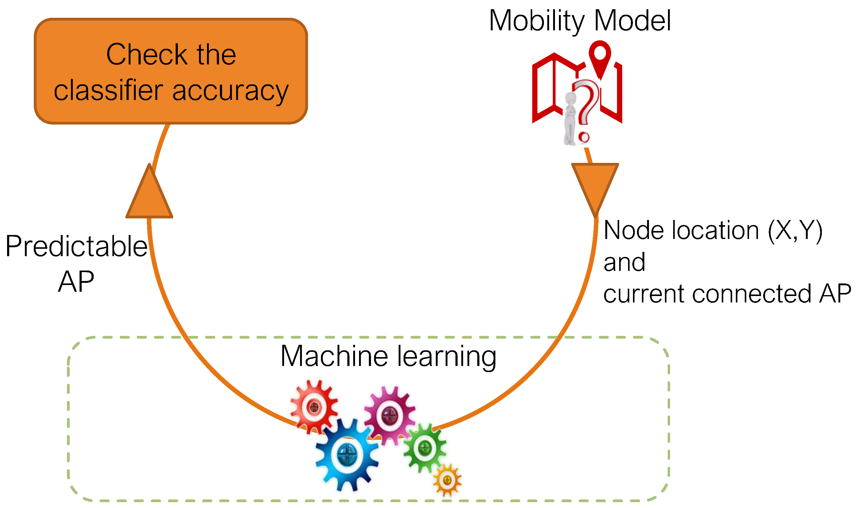
5. Methodology
6. Results and Evaluation
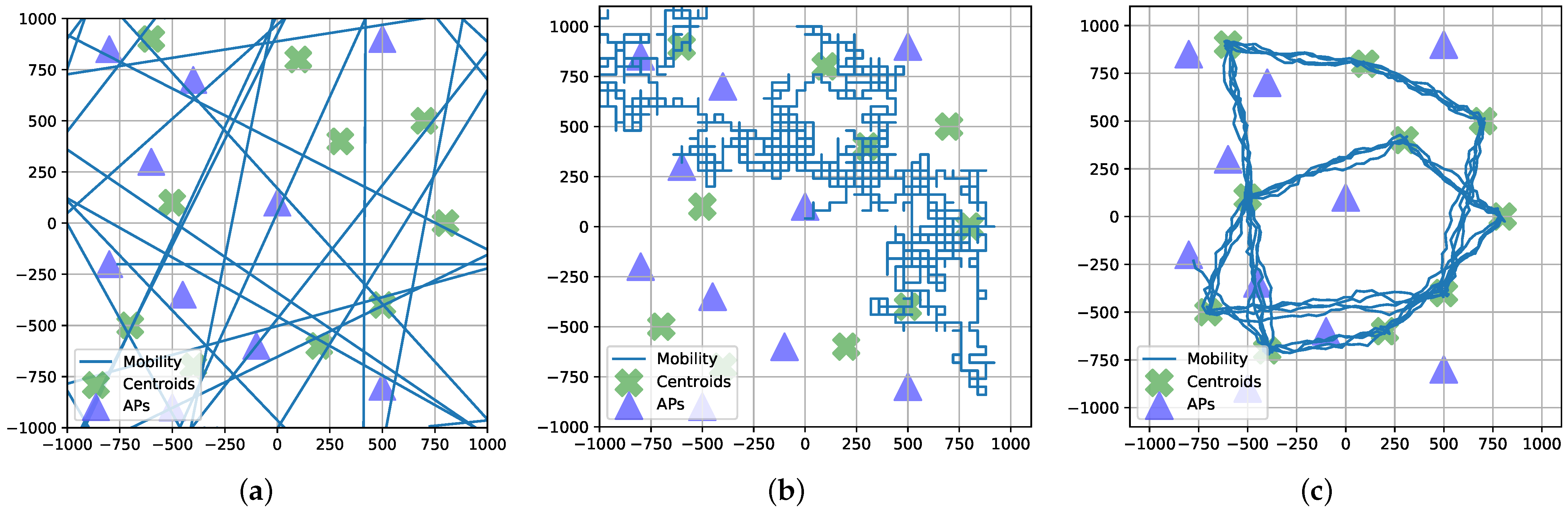
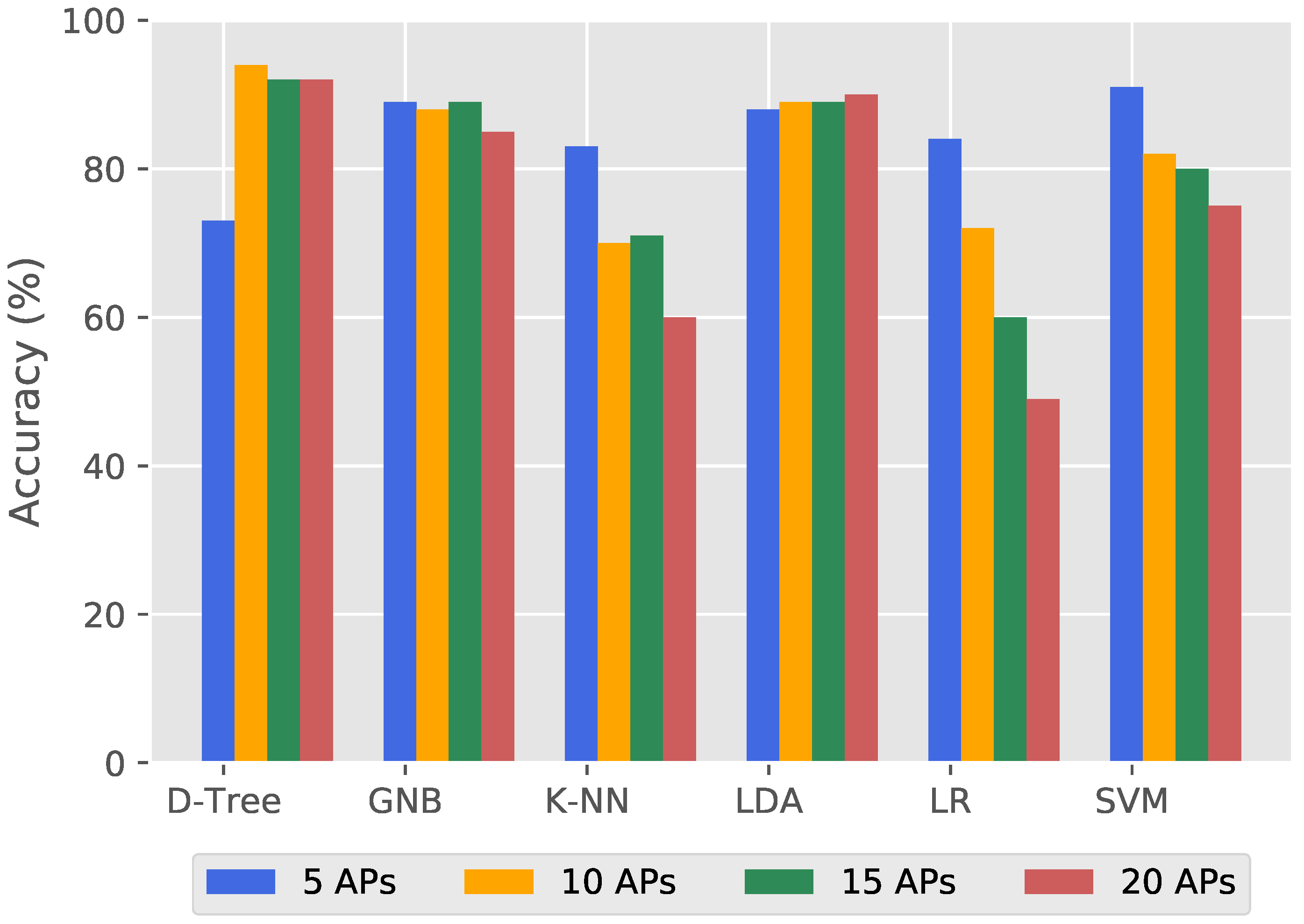
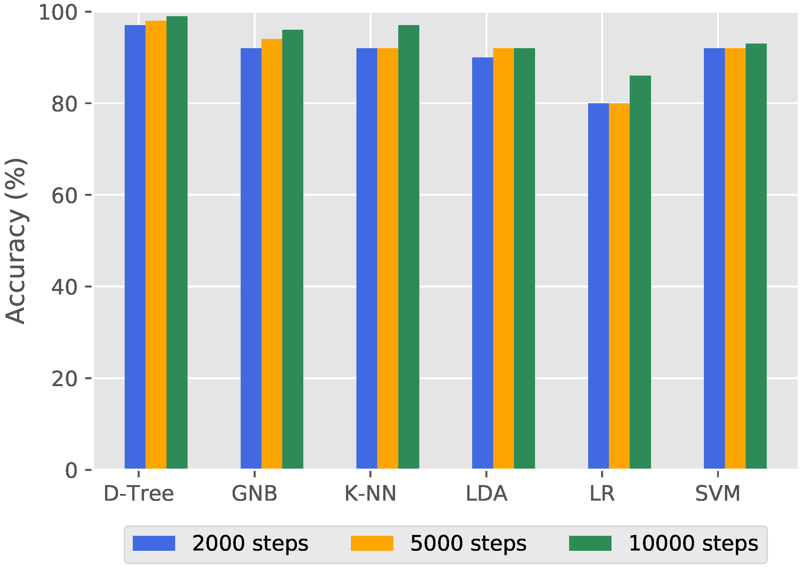
6.1. Evaluation of the RD Mobility Model
6.2. Evaluation of the RW Mobility Model
6.3. Evaluation of the Gauss–Markov Mobility Model
6.4. Evaluation of the RSSGM Mobility Model
7. Discussion and Analysis
8. Conclusions and Future Work
Author Contributions
Funding
Institutional Review Board Statement
Informed Consent Statement
Data Availability Statement
Conflicts of Interest
References
- Alenazi, M.J.F.; Abbas, S.O.; Almowuena, S.; Alsabaan, M. RSSGM: Recurrent Self-Similar Gauss–Markov Mobility Model. Electronics 2020, 9, 89. [Google Scholar] [CrossRef]
- Gebrie, H.; Farooq, H.; Imran, A. What Machine Learning Predictor Performs Best for Mobility Prediction in Cellular Networks? In Proceedings of the 2019 IEEE International Conference on Communications Workshops (ICC Workshops), Shanghai, China, 20–24 May 2019; pp. 1–6. [Google Scholar] [CrossRef]
- Alzoman, R.; Alenazi, M. A Comparative Study of Traffic Classification Techniques for Smart City Networks. Sensors 2021, 21, 4677. [Google Scholar] [CrossRef] [PubMed]
- Gharib, M.; Foroozani, A.; Rezaei, S.; Hemmatyar, A.; Movaghar, A. An Area-Scalable Human-Based Mobility Model. Comput. Netw. 2020, 177, 107300. [Google Scholar] [CrossRef]
- Liang, B.; Haas, Z. Predictive distance-based mobility management for PCS networks. In Proceedings of the IEEE INFOCOM’99. Conference on Computer Communications. Proceedings. Eighteenth Annual Joint Conference of the IEEE Computer and Communications Societies. The Future is Now (Cat. No.99CH36320), New York, NY, USA, 21–25 March 1999; Volume 3, pp. 1377–1384. [Google Scholar] [CrossRef]
- Biomo, J.D.M.M.; Kunz, T.; St-Hilaire, M. An enhanced Gauss–Markov mobility model for simulations of unmanned aerial ad hoc networks. In Proceedings of the 2014 7th IFIP Wireless and Mobile Networking Conference (WMNC), Vilamoura, Portugal, 20–22 May 2014; pp. 1–8. [Google Scholar] [CrossRef]
- Ariyakhajorn, J.; Wannawilai, P.; Sathitwiriyawong, C. A Comparative Study of Random Waypoint and Gauss–Markov Mobility Models in the Performance Evaluation of MANET. In Proceedings of the 2006 International Symposium on Communications and Information Technologies, Bangkok, Thailand, 18–20 October 2006; pp. 894–899. [Google Scholar] [CrossRef]
- Gowda, S.G.; Jacob, S. Network Mobile Topology Impact QOS in Multiservice Manet. Acta Tech. Corvininesis-Bull. Eng. 2020, 13, 79–85. [Google Scholar]
- Khaki, M.; Ghasemi, A. The impact of mobility model on handover rate in heterogeneous multi-tier wireless networks. Comput. Netw. 2020, 182, 107454. [Google Scholar] [CrossRef]
- Bilgin, M. Novel random models of entity mobility models and performance analysis of random entity mobility models. Turk. J. Electr. Eng. Comput. Sci. 2020, 28, 708–726. [Google Scholar] [CrossRef]
- Banagar, M.; Dhillon, H.S. Performance Characterization of Canonical Mobility Models in Drone Cellular Networks. IEEE Trans. Wirel. Commun. 2020, 19, 4994–5009. [Google Scholar] [CrossRef]
- Hossen, M.S.; Rahim, M. Analysis of Delay-Tolerant Routing Protocols using the Impact of Mobility Models. Scalable Comput. 2019, 20, 17–26. [Google Scholar] [CrossRef] [Green Version]
- Norouzi Kandalan, R.; Alla, S.; Rezaeian, N. Impact of Mobility on Consensus Building in the Leader-Follower Model. In Proceedings of the 2019 IEEE 90th Vehicular Technology Conference (VTC2019-Fall), Honolulu, HI, USA, 22–25 September 2019; pp. 1–6. [Google Scholar] [CrossRef]
- Ferreira, L.A.; Guimarães, F.G.; Silva, R. Applying Genetic Programming to Improve Interpretability in Machine Learning Models. In Proceedings of the 2020 IEEE Congress on Evolutionary Computation (CEC), Glasgow, UK, 19–24 July 2020; pp. 1–8. [Google Scholar] [CrossRef]
- Austria, Y.; Goh, M.; Jr, L.; Lalata, J.A.; Goh, J.; Vicente, H. Comparison of Machine Learning Algorithms in Breast Cancer Prediction Using the Coimbra Dataset. Int. J. Simul. Syst. Sci. Technol. 2019. [Google Scholar] [CrossRef]
- Gu, Z.; Wang, J.; Luo, S. Investigation on the quality assurance procedure and evaluation methodology of machine learning building energy model systems. In Proceedings of the 2020 International Conference on Urban Engineering and Management Science (ICUEMS), Zhuhai, China, 24–26 April 2020; pp. 96–99. [Google Scholar] [CrossRef]
- Luo, Y. Uncertainty of the Classification Result from a Linear Discriminant Analysis. In Proceedings of the 2020 IEEE International Workshop on Metrology for Industry 4.0 IoT, Roma, Italy, 3–5 June 2020; pp. 101–105. [Google Scholar] [CrossRef]
- Guo, C.Y.; Chou, Y.C. A novel machine learning strategy for model selections—Stepwise Support Vector Machine (StepSVM). PLoS ONE 2020, 15, e0238384. [Google Scholar] [CrossRef]
- Gupta, A.; Sharma, S.; Goyal, S.; Rashid, M. Novel XGBoost Tuned Machine Learning Model for Software Bug Prediction. In Proceedings of the 2020 International Conference on Intelligent Engineering and Management (ICIEM), London, UK, 17–19 June 2020; pp. 376–380. [Google Scholar] [CrossRef]
- Isak-Zatega, S.; Lipovac, A.; Lipovac, V. Logistic regression based in-service assessment of mobile web browsing service quality acceptability. EURASIP J. Wirel. Commun. Netw. 2020, 2020, 1–21. [Google Scholar] [CrossRef]
- Saber, M.; El Rharras, A.; Saadane, R.; Kharraz, A.H.; Chehri, A. An Optimized Spectrum Sensing Implementation Based on SVM, KNN and TREE Algorithms. In Proceedings of the 2019 15th International Conference on Signal-Image Technology Internet-Based Systems (SITIS), Sorrento, Italy, 26–29 November 2019; pp. 383–389. [Google Scholar] [CrossRef]
- Begum, S.; Chakraborty, D.; Sarkar, R. Data Classification Using Feature Selection and kNN Machine Learning Approach. In Proceedings of the 2015 International Conference on Computational Intelligence and Communication Networks (CICN), Jabalpur, India, 12–14 December 2015; pp. 811–814. [Google Scholar]
- Tan, X. Topic Extraction and Classification Method Based on Comment Sets. J. Inf. Process. Syst. 2020, 16, 329–342. [Google Scholar] [CrossRef]
- Leng, Y.; Zhao, W.; Lin, C.; Sun, C.; Wang, R.; Yuan, Q.; Li, D. LDA-based data augmentation algorithm for acoustic scene classification. Knowl.-Based Syst. 2020, 195, 105600. [Google Scholar] [CrossRef]
- Kamel, H.; Abdulah, D.; Al-Tuwaijari, J.M. Cancer Classification Using Gaussian Naive Bayes Algorithm. In Proceedings of the 2019 International Engineering Conference (IEC), Erbil, Iraq, 23–25 June 2019; pp. 165–170. [Google Scholar]
- Tzanos, G.; Kachris, C.; Soudris, D. Hardware Acceleration on Gaussian Naive Bayes Machine Learning Algorithm. In Proceedings of the 2019 8th International Conference on Modern Circuits and Systems Technologies (MOCAST), Thessaloniki, Greece, 13–15 May 2019; pp. 1–5. [Google Scholar]
- Vapnik, V.N. The Nature of Statistical Learning Theory, 2nd ed.; Springer: Berlin/Heidelberg, Germany, 1999. [Google Scholar]
- Shao, Y.; Yuan, X.; Zhang, C.; Liu, C. Rolling Bearing Fault Diagnosis Based on Wavelet Package Transform and IPSO Optimized SVM. In Proceedings of the 2020 Chinese Control And Decision Conference (CCDC), Hefei, China, 22–24 August 2020; pp. 2758–2763. [Google Scholar]
- Zhao, X.; Yan, X.; Yu, A.; Van Hentenryck, P. Prediction and Behavioral Analysis of Travel Mode Choice: A Comparison of Machine Learning and Logit Models. Travel Behav. Soc. 2020, 20, 22–35. [Google Scholar] [CrossRef]
- Sarao, P. Machine learning and deep learning techniques on wireless networks. Int. J. Eng. Res. Technol. 2019, 12, 311–320. [Google Scholar]
- Alzahrani, A.; Alenazi, M. Designing a Network Intrusion Detection System Based on Machine Learning for Software Defined Networks. Future Internet 2021, 13, 111. [Google Scholar] [CrossRef]
- Alzahrani, A.; Alenazi, M. ML-IDSDN: Machine learning based intrusion detection system for software-defined network. Concurrency and Computation: Practice and Experience 2023, 35, e7438. [Google Scholar] [CrossRef]
- Lin, Z.; Lin, M.; Wang, J.B.; de Cola, T.; Wang, J. Joint Beamforming and Power Allocation for Satellite-Terrestrial Integrated Networks With Non-Orthogonal Multiple Access. IEEE J. Sel. Top. Signal Process. 2019, 13, 657–670. [Google Scholar] [CrossRef] [Green Version]
- An, K.; Lin, M.; Ouyang, J.; Zhu, W.P. Secure Transmission in Cognitive Satellite Terrestrial Networks. IEEE J. Sel. Areas Commun. 2016, 34, 3025–3037. [Google Scholar] [CrossRef]
- Lin, Z.; Niu, H.; An, K.; Wang, Y.; Zheng, G.; Chatzinotas, S.; Hu, Y. Refracting RIS-Aided Hybrid Satellite-Terrestrial Relay Networks: Joint Beamforming Design and Optimization. IEEE Trans. Aerosp. Electron. Syst. 2022, 58, 3717–3724. [Google Scholar] [CrossRef]
- Lin, Z.; An, K.; Niu, H.; Hu, Y.; Chatzinotas, S.; Zheng, G.; Wang, J. SLNR-based Secure Energy Efficient Beamforming in Multibeam Satellite Systems. IEEE Trans. Aerosp. Electron. Syst. 2022, 1–4. [Google Scholar] [CrossRef]
- Lubans, D.R.; Plotnikoff, R.C.; Miller, A.; Scott, J.J.; Thompson, D.; Tudor-Locke, C. Using Pedometers for Measuring and Increasing Physical Activity in Children and Adolescents: The Next Step. Am. J. Lifestyle Med. 2015, 9, 418–427. [Google Scholar] [CrossRef]
- Hishamuddin, M.N.F.; Hassan, M.F.; Tran, D.C.; Mokhtar, A.A. Improving Classification Accuracy of Scikit-learn Classifiers with Discrete Fuzzy Interval Values. In Proceedings of the 2020 International Conference on Computational Intelligence (ICCI), Bandar Seri Iskandar, Malaysia, 8–9 October 2020; pp. 163–166. [Google Scholar] [CrossRef]
- Pedregosa, F.; Varoquaux, G.; Gramfort, A.; Michel, V.; Thirion, B.; Grisel, O.; Blondel, M.; Prettenhofer, P.; Weiss, R.; Dubourg, V.; et al. Scikit-learn: Machine Learning in Python. J. Mach. Learn. Res. 2011, 12, 2825–2830. [Google Scholar]


| APs | X (m) | Y (m) | Centroids | X (m) | Y (m) |
|---|---|---|---|---|---|
| 1 | −800 | −200 | 1 | −400 | −700 |
| 2 | −400 | 700 | 2 | −600 | 900 |
| 3 | 0 | 100 | 3 | 100 | 800 |
| 4 | 500 | 900 | 4 | 700 | 500 |
| 5 | 500 | −800 | 5 | 500 | −400 |
| 6 | −500 | −900 | 6 | −700 | −500 |
| 7 | −450 | −350 | 7 | −500 | 100 |
| 8 | −100 | −600 | 8 | 300 | 400 |
| 9 | −600 | 300 | 9 | 800 | 0 |
| 10 | −800 | 850 | 10 | 200 | −600 |
| 11 | −100 | 950 | 11 | −200 | −200 |
| 12 | 900 | 600 | 12 | −800 | 400 |
| 13 | 500 | 400 | 13 | 800 | −800 |
| 14 | 850 | 250 | 14 | −100 | 500 |
| 15 | 300 | −200 | 15 | 200 | 0 |
| 16 | 200 | −850 | 16 | −900 | −900 |
| 17 | 700 | −500 | 17 | −100 | −900 |
| 18 | −300 | 0 | 18 | 500 | 100 |
| 19 | 100 | 550 | 19 | 900 | −400 |
| 20 | −900 | −700 | 20 | −900 | 700 |
| Time (s) | X (m) | Y (m) | Previous AP | Current AP |
|---|---|---|---|---|
| 32 | −522.039 | 234.0297 | 0 | 1 |
| 33 | −534.758 | 282.532 | 1 | 1 |
| 34 | −545.7 | 331.5814 | 1 | 1 |
| 35 | −551.134 | 381.5525 | 1 | 1 |
| 36 | −560.975 | 430.9473 | 1 | 1 |
| . | ||||
| . | ||||
| . | ||||
| 467 | 149.2532 | 660.1039 | 2 | 3 |
| 468 | 114.1719 | 625.27 | 3 | 3 |
| 469 | 76.80538 | 593.0601 | 3 | 1 |
| 470 | 39.04904 | 561.3788 | 1 | 1 |
| 471 | 5.846693 | 524.811 | 1 | 2 |
| 472 | −25.0253 | 486.2131 | 2 | 2 |
| 473 | −18.7087 | 535.4928 | 2 | 1 |
| 474 | −1.68525 | 582.249 | 1 | 1 |
| 475 | 23.00982 | 625.3539 | 1 | 1 |
| 476 | 45.7389 | 669.5808 | 1 | 1 |
| 477 | 58.65014 | 717.8236 | 1 | 1 |
| 478 | 75.00265 | 764.9371 | 1 | 3 |
| 479 | 86.98774 | 813.4452 | 3 | 3 |
| 480 | 132.711 | 793.1574 | 3 | 3 |
| . | ||||
| . | ||||
| . | ||||
| 799 | 680.0722 | 395.8155 | 2 | 3 |
| 800 | 628.7113 | 401.9032 | 3 | 3 |
Publisher’s Note: MDPI stays neutral with regard to jurisdictional claims in published maps and institutional affiliations. |
© 2022 by the authors. Licensee MDPI, Basel, Switzerland. This article is an open access article distributed under the terms and conditions of the Creative Commons Attribution (CC BY) license (https://creativecommons.org/licenses/by/4.0/).
Share and Cite
Abbas, S.; Alenazi, M.J.F.; Samha, A. Mobility Prediction of Mobile Wireless Nodes. Appl. Sci. 2022, 12, 13041. https://doi.org/10.3390/app122413041
Abbas S, Alenazi MJF, Samha A. Mobility Prediction of Mobile Wireless Nodes. Applied Sciences. 2022; 12(24):13041. https://doi.org/10.3390/app122413041
Chicago/Turabian StyleAbbas, Shatha, Mohammed J. F. Alenazi, and Amani Samha. 2022. "Mobility Prediction of Mobile Wireless Nodes" Applied Sciences 12, no. 24: 13041. https://doi.org/10.3390/app122413041