


Ultrasonic Attenuation of Ceramic and Inorganic Materials Using the Through-Transmission Method

Department of Materials Science and Engineering, University of California, Los Angeles (UCLA), Los Angeles, CA 90095, USA
Appl. Sci. 2022, 12(24), 13026; https://doi.org/10.3390/app122413026
Submission received: 24 November 2022
/
Revised: 14 December 2022
/
Accepted: 15 December 2022
/
Published: 19 December 2022
(This article belongs to the Topic Recent Advances in Structural Health Monitoring)
Abstract
:Ultrasonic attenuation coefficients of ceramic and inorganic materials were determined for the longitudinal and transverse wave modes. Sample materials included hard and soft ceramics, common ceramics, ceramic-matrix composites, mortars, silicate glasses, rocks, minerals and crystals. For ceramic attenuation measurements, a standardized method has existed, but this method based on a buffer-rod arrangement was found to be inconsistent, producing vastly different results. Resonant ultrasound spectroscopy was also found to be unworkable from its sample preparation requirements. Experimental reevaluation of the buffer-rod method showed its impracticality due to unpredictable reflectivity parameters, yielding mostly negative attenuation coefficients. In this work, attenuation tests relied on a through-transmission method, which incorporated a correction procedure for diffraction losses. Attenuation exhibited four types of frequency (f) dependence, i.e., linear, linear plus f4 (called Mason-McSkimin relation), f2 and f3. The first two types were the most often observed. Elastic constants of tested materials were also tabulated, including additional samples too small for attenuation tests. Observed levels of attenuation coefficients will be useful for designing test methods for ultrasonic nondestructive evaluation and trends on ultrasonic attenuation are discussed in terms of available theories. However, many aspects of experimental findings remain unexplained and require future theoretical developments and detailed microstructural characterization. This study discovered a wide range of attenuation behaviors, indicating that the attenuation parameter can aid in characterizing the condition of intergranular boundaries in combination with imaging studies.
1. Introduction
Ultrasonic methods of nondestructive evaluation (NDE) have been used on ceramic and inorganic materials and structures for 70 years [1,2]. The oldest and most widely used among them was to empirically estimate concrete strength by measuring the velocity of longitudinal waves, known as the ultrasonic pulse velocity method. This was developed in Canada in the 1940s and relied on a pulse-transmission technique [3], which was a variation of Firestone’s pulse-echo method, patented in 1942 [4]. Despite its long history, it is still actively studied and effects of various parameters are characterized, see for example, [5]. Another well-established approach is based on the correlation between the porosity of ceramics and their ultrasonic velocities of the longitudinal and transverse waves [6]. The porosity-velocity relationship is backed by various theoretical analyses [7]. Another NDE method that depends on elastic wave propagation is called acoustic emission (AE), which passively listens to acoustic signals emanating from developing flaws in a structure under load. Again, AE methods are used more often in concrete and their current status can be found in [8]. In recent NDE studies of ceramic-matrix composites, AE monitoring achieved striking successes, characterizing damage growth under tensile and stress-rupture loading at elevated temperatures [9]. Still, there are numerous applications of ceramic and inorganic materials, which can benefit from expanded uses of ultrasonic NDE. For example, carbon–carbon (C-C) composite brake discs can gain an increased lifetime with proper NDE. Air-coupled ultrasonic NDE reports are promising for wider practical uses.
In all the ultrasonic NDE applications, it is necessary to know ultrasonic properties of a material under test in order to optimize ultrasonic NDE procedures. While ultrasonic velocities of the longitudinal and transverse waves are readily available in published tables or by standardized testing for many engineering materials, attenuation coefficients were difficult to measure and were obtained only for limited materials. These materials included metals, ceramics, polymers and rocks. Mason and McSkimin [10] were the first to measure the ultrasonic attenuation of a metal (pure magnesium) using a pulse propagation method. See classical treatises [11,12] and a review [13] for early development. Available attenuation data on metals and composites was collected in [14]. There are many reports on the attenuation of geologic materials. While the frequency range is mostly at or below the audio frequencies, some reports extended to the low-MHz region, as assembled in [13,15,16]. Some of the geologic attenuation studies relied on substitution methods, comparing aluminum and rock samples, but without accounting for beam spread and diffraction losses, as will be discussed later. Resonant ultrasound spectroscopy (RUS) has been the preferred method [17,18,19]. RUS obtains the resonance spectra of samples of defined shapes, such as spheres, cubes and parallelepipeds. These are then compared to calculated natural frequencies with approximate elastic constants, followed by the application of a nonlinear inversion algorithm in order to deduce the elastic constants of the samples. Initially, spherical samples were used; e.g., on tektites and moon rocks [20,21]. RUS was then expanded to cubes and parallelepipeds [22,23,24,25], enabling the determination of the elastic constants of anisotropic solids [23,24,26]. Damping factors (or Q−1) can be obtained by determining the broadening of the resonance peaks [17,18,19,21]. The main drawback of RUS is elaborate sample preparation. For hard ceramic and porous materials, the preparation of precise shapes is difficult and expensive, making RUS highly impractical for NDE applications. Another issue is its inability to obtain transverse-wave attenuation since an RUS sample is dry-coupled to transducers. In fact, damping factors obtained with RUS appear to contain varied fractions of transverse-attenuation contribution, since most vibration modes cannot be purely extensional. This implies that the theoretical basis of RUS-based attenuation measurements needs to be reexamined. Additionally, Balakirev et al. [19] specified that sample materials for RUS need to possess Q values of several hundreds, implying damping factors of less than 0.003. This condition is especially restrictive for hard engineering materials if applicable for damping study. In polymer damping studies, RUS yielded satisfactory results, covering a wide frequency range [27,28,29] since sample preparation presented no hurdle and the use of larger sample sizes apparently overcame the damping factor restriction.
The standardized method of attenuation measurement of advanced ceramics, ASTM C1332-18 [30], utilized the buffer-rod method by Papadakis [31,32]. Evans et al. [33] used this method for several advanced ceramics, SiC, Si3N4, MgO, ZnS and lead zirconate-titanate (PZT). Generazio and others further developed the method for the ASTM C1332 standard document [34,35,36]. Additionally, Papadakis [32] provided attenuation data for graphite (ATJ grade) and ASTM C1332 document included cobalt-bonded WC cermet data [30]. The applicability of this C1332 method to materials other than advanced ceramics appears to be limited, since the center frequency of input pulse was specified to be 50 MHz or higher. Thus, no report of its usage can be found in the literature. Additionally, the validity of this method is questionable since there existed vast differences in the attenuation values reported for SiC and Si3N4 in [33] and [34,35,36]. Both groups used the same buffer-rod method, and the values were expected to be comparable. However, for Si3N4, Evans et al. [33] obtained attenuation coefficients ranging from 150 to 5300 dB/m at 11 to 53 MHz. In contrast, Generazio [34] reported 235 dB/m at 60 MHz and Roth et al. [36] reported 130 to 1020 dB/m at 30 to 110 MHz (with 480 or 696 dB/m at 50 or 60 MHz). These results from two distinguished laboratories revealed large discrepancies of more than a factor of ten, highlighting the difficulty of the buffer-rod method. Several reports of PZT attenuation testing also showed a wide data spread as in Si3N4. Evans et al. [33] found the attenuation of PZT at 10 MHz to be 565 dB/m. This was close to 550 dB/m by Truell et al. [37] and to 590 dB/m by Kuscer et al. [38] and was within the range of 40 to 600 dB/m by Jen et al. [39], all at 10 MHz. In contrast, Na and Breazeale [40] obtained 28 to 115 dB/m, while Wang et al. [41] reported 1570 dB/m for PZT-5H, also at 10 MHz. The methods used and sample PZT compositions varied, but the PZT results were not close to a consensus and the low values from [40] were comparable to those of aluminum alloys [37], known to be among the lowest attenuating materials. From the above comparisons of attenuation data from various sources, it is evident that wide ranges of attenuation coefficients and their frequency dependencies reflect the lack of reliable test methods. In particular, the buffer-rod method, including the more restrictive ASTM C1332-18 standard [30,31,32], needs to be reexamined for its validity and reliability.
The difficulties of the buffer-rod method appear to arise from the use of reflection coefficients in calculating attenuation and wave refraction occurring at the buffer-sample interface. Treiber et al. [42] recognized the difficulty of getting consistent reflection coefficients and devised a sequence of eight contact tests to determine them. They measured attenuation coefficients of polymethyl methacrylate (PMMA) and the results matched published values well. However, their results for cement paste vanished below 0.9 MHz, indicating needs for reevaluation. Still, the eight-step testing is difficult to implement except for research purposes. In the following section, the practicality of the buffer-rod method will be examined.
Another method for attenuation measurement using differential transmission was recently introduced [43,44]. This method was a derivative of the widely used approximate procedure of ASTM E664 [45], adopting the contact method of the buffer-rod method in lieu of the immersion method (that generates unwanted refraction at the water-sample boundaries). The attenuation due to the presence of coupling layers was accounted for by the use of samples of different thicknesses. In addition, it incorporated the correction for diffraction loss [46] using an analytic expression [47]. By using the simplified procedures, the number of materials with longitudinal and transverse ultrasonic attenuation coefficients increased by more than 200 [43,44]. However, the number of ceramic and inorganic materials with both longitudinal and transverse attenuation coefficients was limited to 24.
In this report, additional measurements of ultrasonic attenuation coefficients were conducted on samples that were too large previously to determine transverse attenuation coefficients and other materials new to this study, increasing the total number of tested ceramic and inorganic materials to 74. These are intended to give guidelines for optimizing ultrasonic NDE procedures of the materials tested here or similar ceramic and inorganic materials. The transmission method used in this study is less demanding, although better surface preparation minimizes overestimates of attenuation coefficients. Additionally, this paper will report ultrasonic velocities and elastic constants of 11 samples that were too small to obtain attenuation coefficients. Experimental methods will be briefly presented. Observed trends on ultrasonic attenuation coefficients will be discussed. While physical mechanisms causing attenuation require further studies, especially concerning the differences between the longitudinal and transverse attenuation and similarities of damping factors among diverse ceramic materials, the present survey establishes the basis for a better understanding of ultrasonic attenuation of ceramic and inorganic materials.
2. Buffer-Rod Method
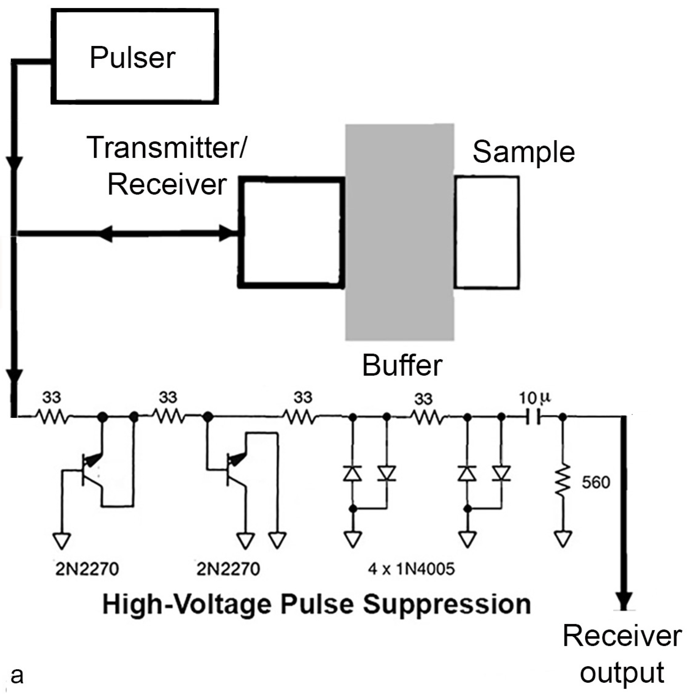
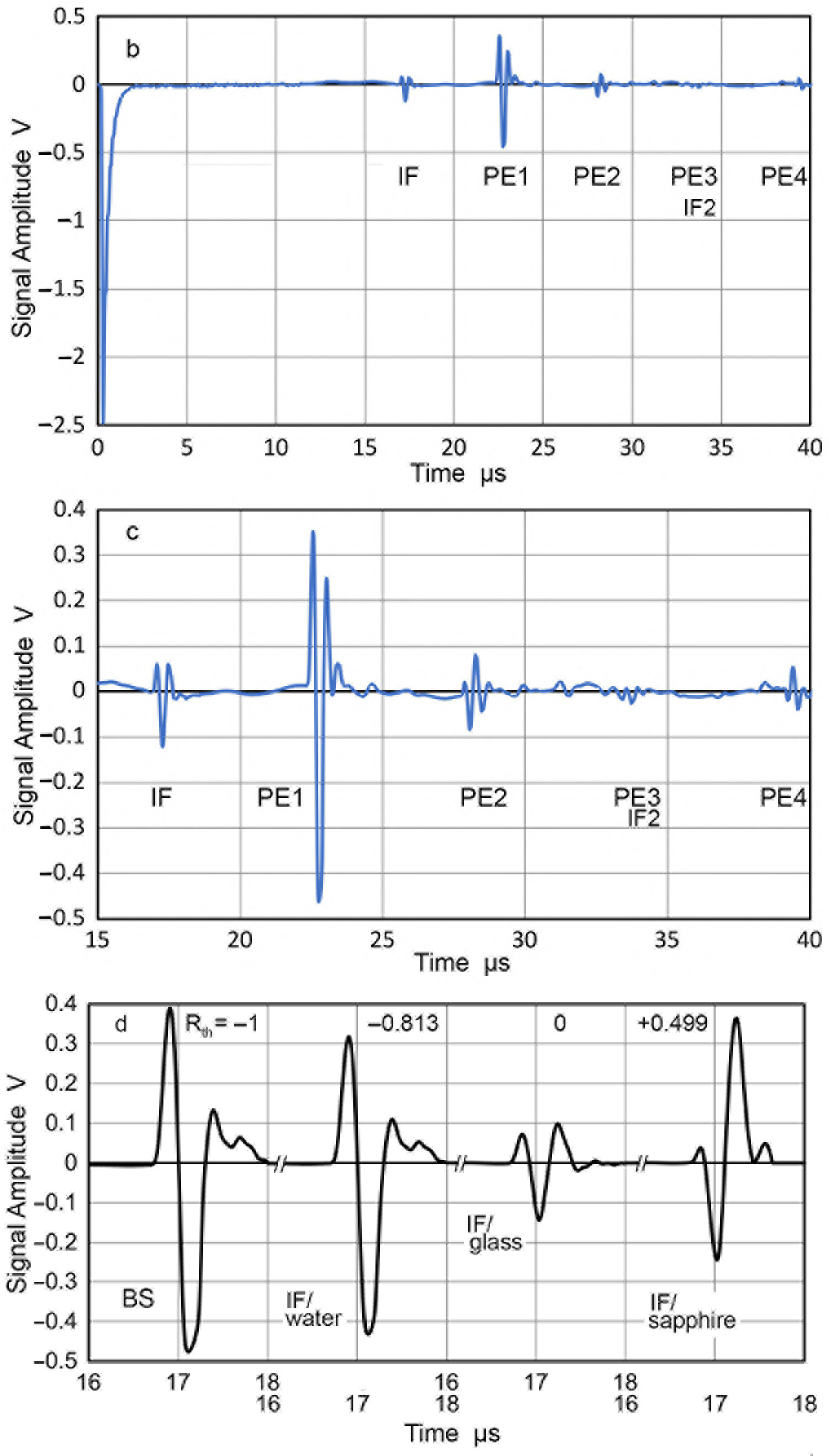
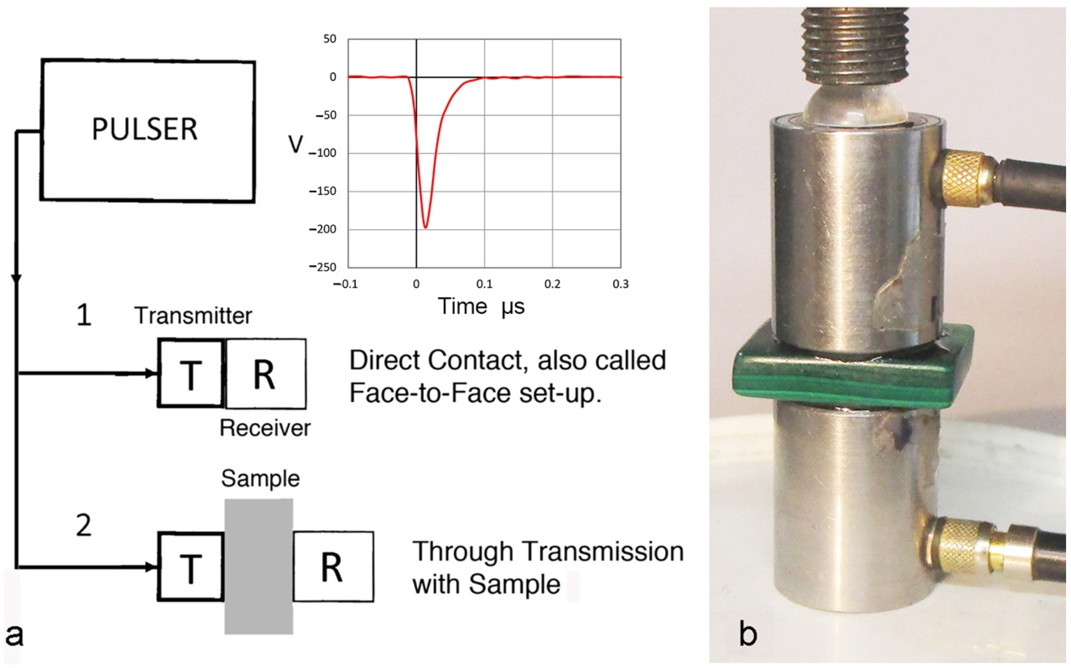
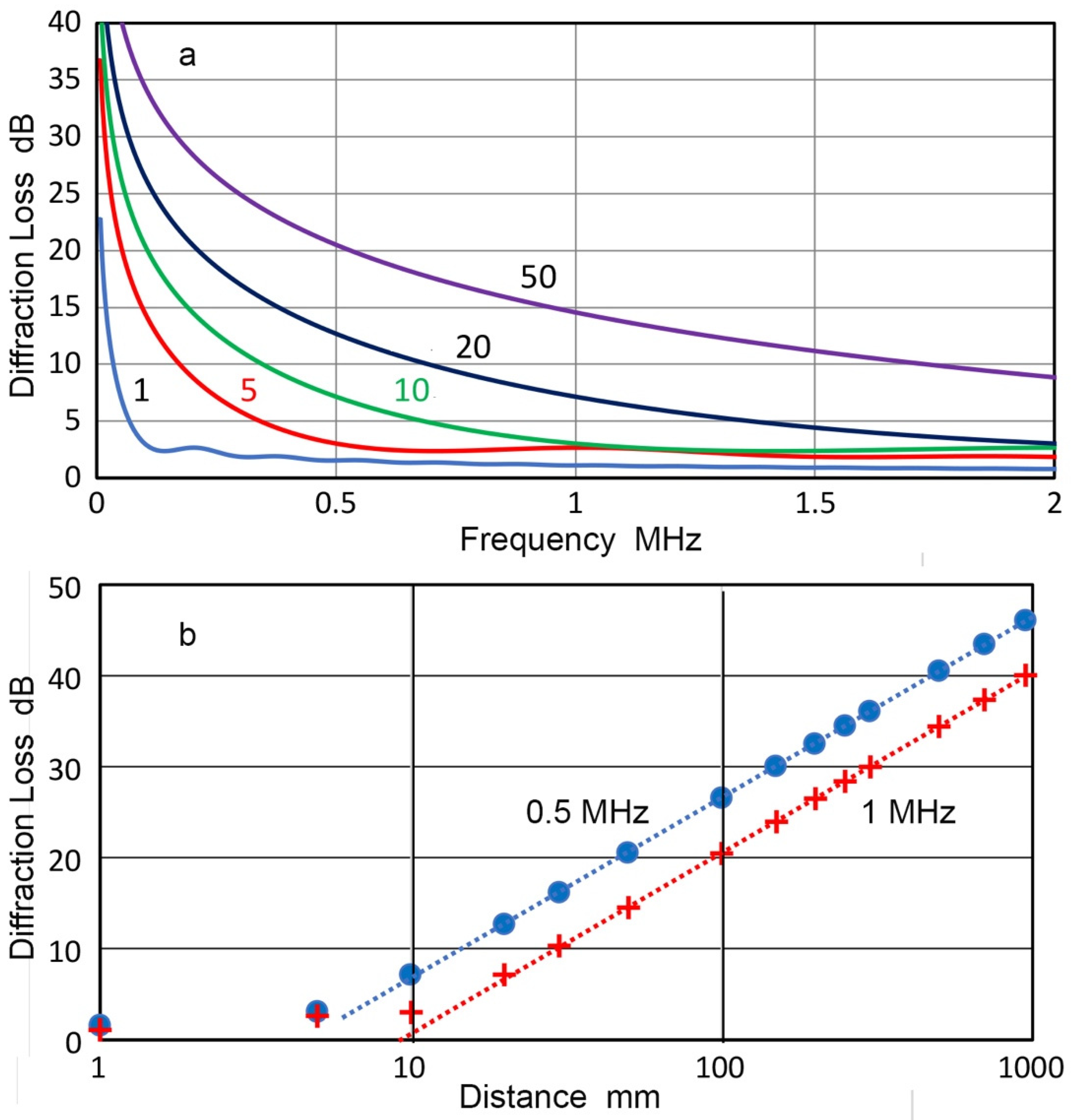
Attenuation measurement using the buffer-rod method [30,31,32] relied on a pulse-echo test set-up, similar to those for ultrasonic flaw detection and ASTM E662 [45]. A buffer plate (or rod) is added as schematically shown in Figure 1a. In this set-up, a high-voltage pulse suppression circuit [48] was inserted between the pulser output and a digital oscilloscope input, producing a wave train of the first interfacial reflection (marked IF in Figure 1b), the first to fourth pulse echo signals (PE1 to PE4) and the second interfacial reflection (IF2). Here, PE3 and IF2 overlapped, reducing both of their amplitudes. The detected signal waveforms are shown in Figure 1c in an enlarged scale. When the sample was absent, the reflection signal from the back surface (BS) of the buffer plate was larger, reaching 0.86 V peak-to-peak (Vpp), whereas the IF signal had 0.19 Vpp (a reduction of 4.5 times corresponding to an amplitude-based reflection coefficient of 0.22 at 1.8 MHz). The BS reflection waveform is shown in Figure 1d. Test conditions were as follows: Transducer, Olympus V104 (2.25 MHz, 25.4 mm diameter, Olympus NDT, Waltham, MA, USA); Buffer plate, BK7 glass, 48.6 mm thickness; Fused silica sample, 16.0 mm thickness, Pulser output voltage, −250 V; Couplant, a petroleum gel (Vaseline). Receiver output was fed to PicoScope 5242D (Pico Technology, St. Neots, UK) and digitized at 8 ns interval with 15-bit resolution, using signal-averaging mode. Fast Fourier transform (FFT) was performed with Noesis software (Enviroacoustics, Athens, Greece, ver. 5.8). For more details, see [43,44].
Frequency dependent reflection coefficient, R(f), is given by
R(f) = F(f)/Fo(f)
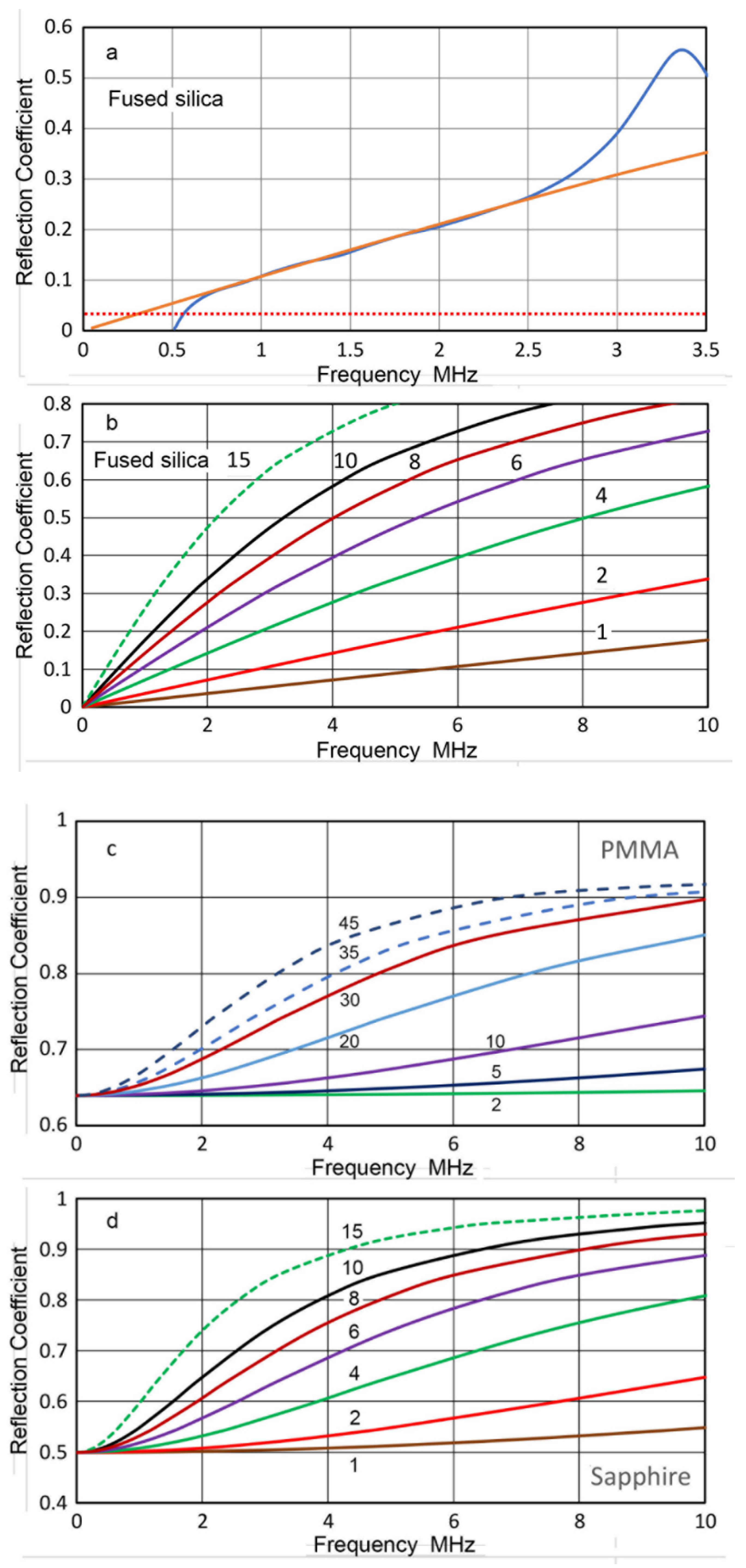
According to the ASTM C1332 standard with F(f) and Fo(f) being power spectra of IF and BS reflections. For the case of the fused silica sample and BK7 glass buffer plate, R(f) is plotted in Figure 2a along with the theoretical reflection coefficient (Rth), plotted in a red dotted line. Rth is frequency independent and is given by
where Zb and Zs are the acoustic impedance of buffer plate and sample, respectively [1]. Note that R(f) by Equation (1) represents its magnitude as the phase component was ignored, while Rth varies from −1 to +1. The sign of Rth reveals itself in the reflected waveform, as can be seen in Figure 1d. The BS wave with Rth = −1 and IF wave from water-backing (Rth = −0.813) have a positive–negative peak sequence. For the glass–sapphire interface (Rth of 0.499), the major peak sequence is reversed to negative–positive type, ignoring the initial minor peak. That is, the phase of the reflected waves was inverted, corresponding to the sign change [1]. Observed R(f) deviated substantially from the theoretical value and the difference increased with frequency. Generazio [34] found similar, but smaller increases for the case of the quartz and nickel combination. As Zb = 14.6 Mrayl and Zs = 12.9 Mrayl are close and are 10 and 9 times Zc of couplant (Z = 1.43 Mrayl), the R(f) can be calculated using an equation from Krautkramer [1], namely,
where m = Zb/Zc, d = couplant thickness, and vc = wave velocity of the couplant, respectively. R(f) values for seven thicknesses (d of 1 to 15 µm) are plotted in Figure 2b, assuming Zb ≈ Zs. For the case of Zb ≠ Zs, Generazio [34] used a similar equation for R(f) with additional terms from Kinsler [49]. Figure 2b shows increasing R(f) as d and f increase. R(f) for d = 6 µm is also plotted in Figure 2a with an orange curve, which matches the observed values of R(f) from 0.7 to 2.5 MHz. The good match between calculated and observed R(f) values indicates an apparent couplant thickness of 6 µm for the glass-fused silica interface. Since both components had optically flat surfaces, this d value appeared to exceed the interfacial spacing and additional tests were conducted.
Rth = (Zs − Zb)/(Zb + Zs)
R(f) = {(0.25(m − 1/m)2 sin2(2πdf/vc))/(1 + 0.25(m − 1/m)2 sin2(2πdf/vc))}0.5
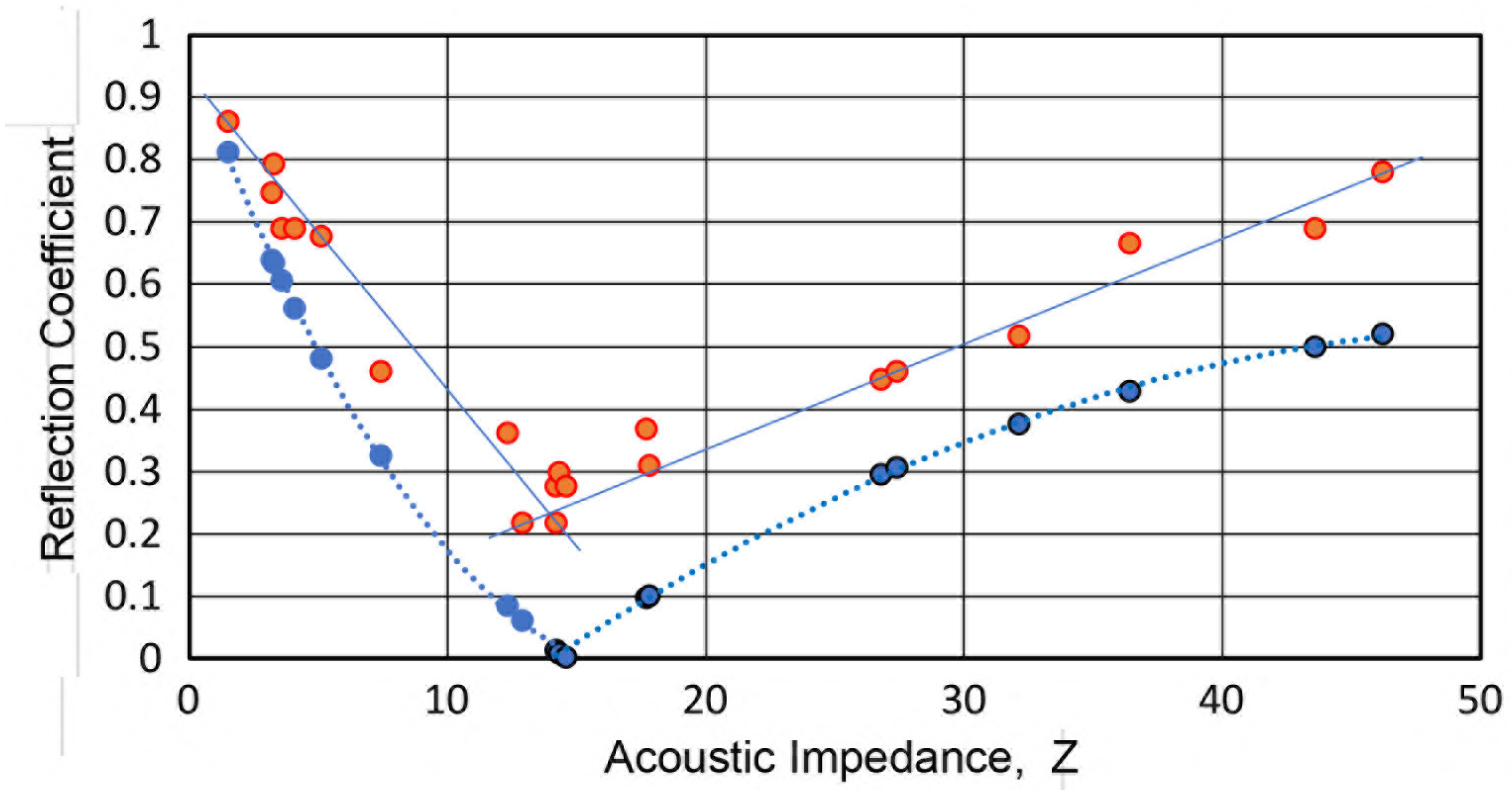
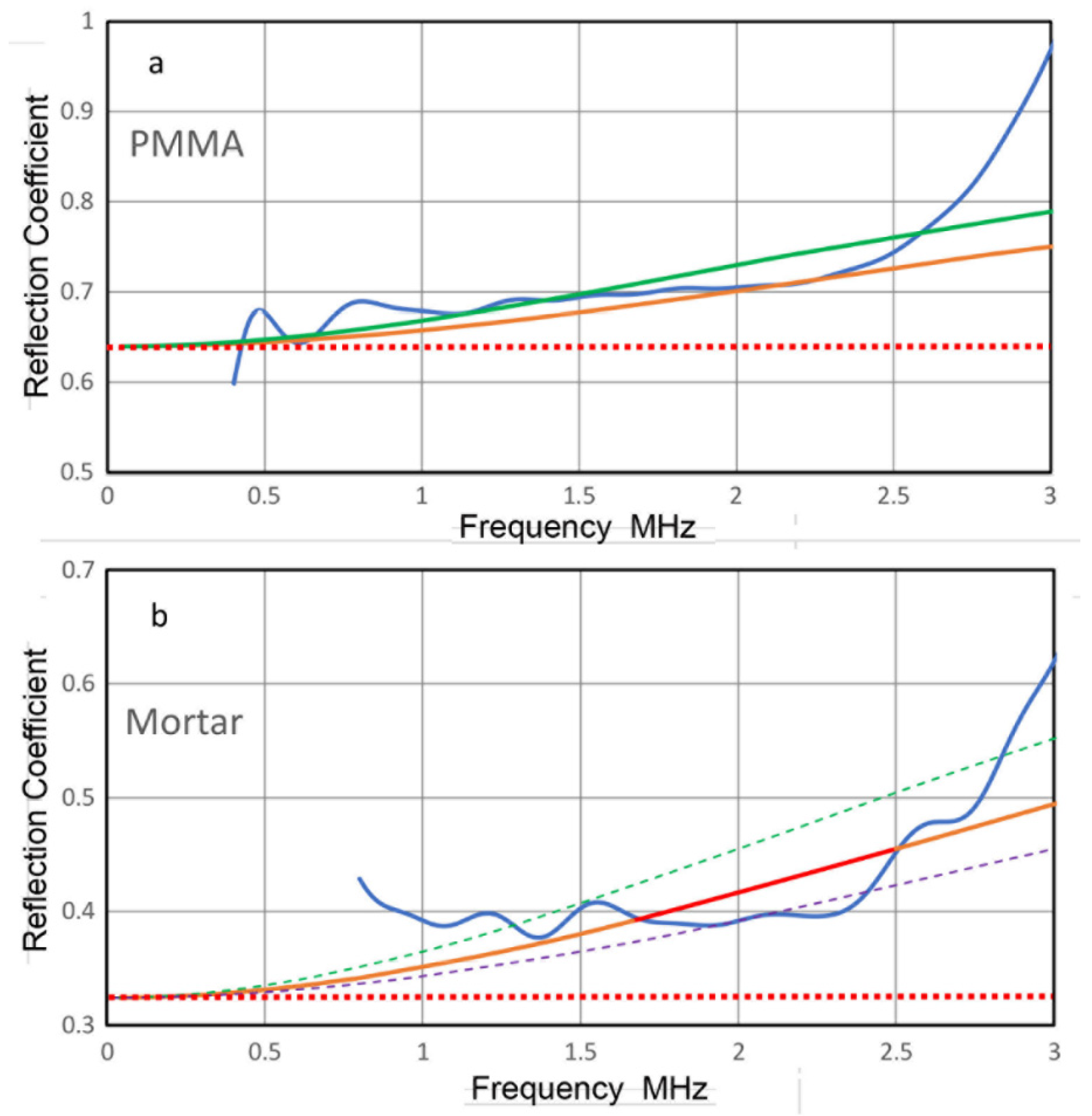
The amplitude-based reflection coefficients of 21 different materials were determined and are plotted with red dots against their Z values in Figure 3. Materials used and their Z and R values are listed in Table 1. The observed R values decreased with Z initially, then increased above Z = 14.6 for the buffer material. Calculated R values are also given with blue dots, which can be fitted to two polynomials for above and below Z = 14.6 of BK7 glass buffer plate. In most cases examined, the observed R values were approximately 0.2 higher than the calculated values and actual differences ranged from 0.05 to 0.3. Since the BS and IF signals had the center frequency near 1.8 MHz, the observed amplitude-based R values approximately represent R(f) at this frequency. This series of tests establishes that the observed amplitude-based R values always differ from the calculated ones.
Using the BS and IF signals for the tests of amplitude-based R values, R(f) values were obtained and six representative plots are shown in Figure 4. The sample materials were polymethyl methacrylate (PMMA), mortar, granite, BK7 glass, alumina and sapphire. All showed the same trend as that of Figure 2b. That is, the observed R values mostly exceeded the calculated R (shown by red dotted lines) with frequency-dependent increase.
For samples with differing Z from that of the buffer, an equation for R(f) is given as,
where n = Zc/Zs and p = Zb/Zs, along with m = Zb/Zc, d = couplant thickness, and vc = wave velocity of the couplant, respectively [34,49]. Two cases for PMMA and sapphire samples were calculated and their R values were plotted in Figure 2c,d for various couplant thicknesses of 2 to 45 and 1 to 15 µm, respectively. For PMMA, the observed R(f) was between calculated R(f) values for couplant thicknesses of 35 and 45 µm, as shown in Figure 4a. This indicated that d = 40 µm provided a good match between the observed and calculated R(f). Figure 4f shows a good match exists with d = 4 µm for the case of glass-sapphire interface. For four other cases of mortar, granite, glass and alumina, calculated R(f) curves of nearly matching d values were plotted with observed R(f) in Figure 4b,e. For mortar, granite, glass and alumina, matching apparent d-values were 12, 10, 7 and 8 µm, while the corresponding d values for fused silica, PMMA and sapphire were 6, 40 and 4 µm, respectively.
R(f) = {((1 − p)2 cos2(2πdf/vc) + (n − m)2 sin2(2πdf/vc))/((1 + p)2 cos2(2πdf/vc) + (n + m)2 sin2(2πdf/vc))}0.5,
The couplant thickness was measured using pairs of well-polished discs and plates of fused silica, sapphire, Pyrex glass, hardened steel and PMMA, with a 1-µm resolution micrometer (as nm-resolution devices were unavailable). For ten combinations, the sum of thickness measurements of individual discs or plates and combined thickness with couplant were identical. That is, the couplant thickness was undetectable in all the combinations tested. Thus, the physical thickness was estimated to be 1 µm, which was the resolution of the micrometer used. Consequently, all seven apparent d values exceeded the estimated couplant thickness by the factor of 4 to 40. The factor was the lowest for sapphire and the highest for PMMA.
Large differences between the physical and apparent d-values are difficult to attribute to errors in micrometer measurements when the difference is more than several µm. It is improbable for the case of PMMA. Thus, it is needed to explore other causes for the differences. A possible source of higher R(f) is the non-planar nature of waves arriving at the buffer-sample interface. Theoretical R(f) calculations [1,49] relied on the planar wave assumption. For the sound field from a circular transmitter (also called a piston source), it is necessary to include the contributions of non-planar reflection and wave refraction when Z value changes at the interface. Thus, the use of R(f) in attenuation testing per the ASTM C1332 demands more detailed analysis of waves impinging on the buffer-sample interface. No such analysis is available at present.
In all the cases examined, R(f) values can be attributed to the interfacial structure even though exact analysis is unavailable. The apparent d-values were deduced from the observed R(f) but appear to exceed the estimate of physical d values, which were within the micrometer resolution.
As shown in Figure 1b,c, reflections from the back surface of a sample can be detected and were designated as PE1, PE2, etc. The ASTM C1332 method calculates power spectra of PE1 and PE2 reflections, B1(f) and B2(f) (in dB). Then, ultrasonic attenuation, α (in dB/m) is given by
where X is sample thickness, and D1(f) and D2(f) are diffraction correction terms (in dB). The D terms were omitted in ASTM C1332 method since it was intended for the high-frequency range above 10 MHz, where these can be ignored. D is given by
where s = xv/f a2, with x being the propagation distance from a transmitter of radius, a. J1 represents the Bessel function of the first kind. This is due to Rogers and van Buren [47], who integrated the Lommel integral for a circular piston motion, received over the same sized area, located at distance x away. For pulse-echo tests, the propagation distance corresponds to a multiple of twice the sample thickness, or 2X. It should be noted that the available calculation of diffraction correction cannot be applied to cases with a buffer-sample interface with a discontinuity in Z. In fact, waves pass the interface twice. When attenuation is high, and transducer size is much larger than the wavelength, effects can be minimized, but proper consideration is required. The diffraction correction analysis also assumed that the propagation medium is uniform. That is, no interface exists where Z value changes stepwise, resulting in wave refraction. Thus, the D terms can only be used as approximation. Even when diffraction effects are small, wave refraction persists and this needs to be included in pulse-echo analysis, although this point has not been considered previously.
α = {B1(f) + |D1(f)| + R(f) − B2(f) − |D2(f)|}/2X
D = 20 log{[cos(2π/s) − J1(2π/s)]2+ [sin(2π/s) − J1(2π/s)]2}0.5
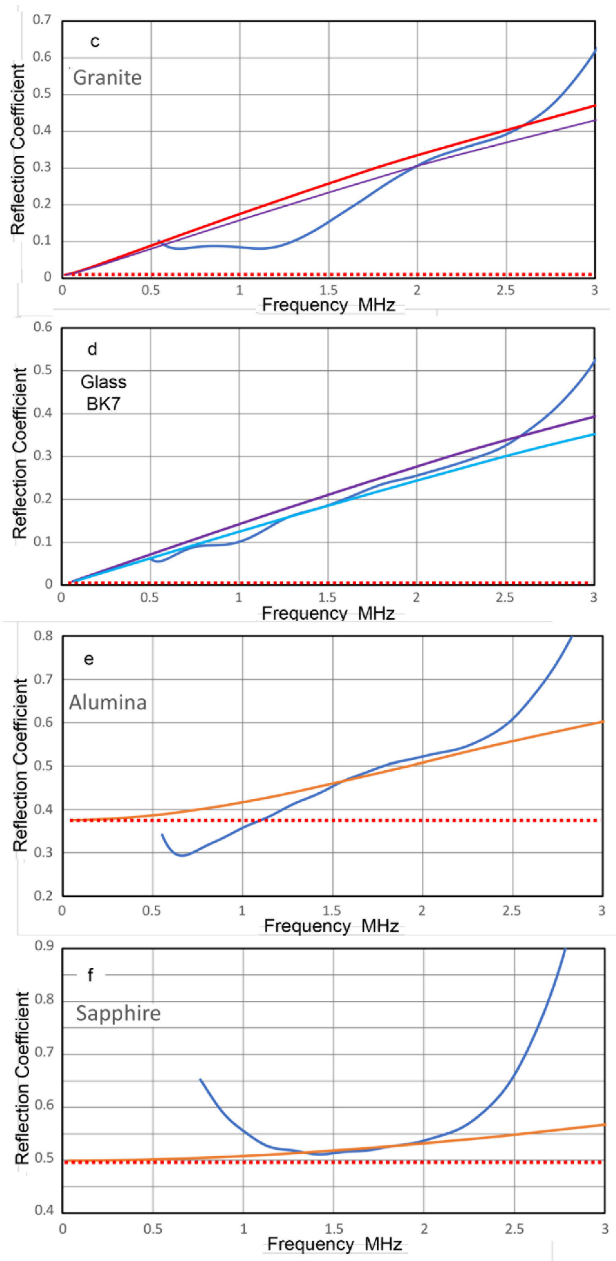
When the buffer-rod method was applied to eight tests, from which B1(f), B2(f) and R(f) data were obtained, only one test for PMMA produced consistently positive attenuation. In all others, attenuation was irregular and often showed only negative α values that cannot exist. The PMMA attenuation results are shown in Figure 5a,b. Figure 5a shows B1(f), B2(f), R(f), |D1(f) − D2(f)| and 2X α plotted against f (in blue, red, purple, brown and green curves, respectively), while Figure 5b gives a plot of α vs. f (in green curve). In both plots of green curves, a sharp rise above 2.5 MHz is due to the increase in R(f) and a slope change at 3 MHz (cut off in Figure 5b) is from the removal of positive R(f) (in dB unit). Additionally, shown in Figure 5b is a blue line for α vs. f from the previous study with the slope of 91.4 ± 4.9 dB/m/MHz [43]. This comparison indicates that the buffer-rod method resulted in a slope of 145 dB/m/MHz (in green dotted line), or two-third higher than the earlier data (blue line). Additionally, plotted in this figure with a red curve is the attenuation result from the use of B1(f) of two sample thicknesses, which enables one to avoid the use of R(f) parameter. For this method, α is given by
where * indicates values for the thicker sample. The attenuation from the two-thickness method (in red curve) is closer to the blue line, and the slope of the fitted line (red dotted line) is 19% higher at 109 dB/m/MHz than that of the blue line. This value is still outside the standard deviation of PMMA attenuation [43] but agrees with the value of 111 dB/m/MHz, reported by Treiber at al. [42]. These results indicates that PE1 signals (or B1(f)) can be useful in attenuation testing. Under field conditions, the access to the back-side of a sample is often unavailable and the pulse-echo techniques are valuable alternatives.
α = {B1(f) − B1*(f) − (|D1*(f)| − |D1(f)|)}/2(X* − X),
Figure 5c provides α vs. f plots of other seven cases that produced adequate PE2 signals. Three solid curves were for fused silica and glasses, dotted curves were for metals and the dashed curve was for polyvinyl chloride (PVC). The PVC curve shows α/10 vs. f for comparison. These results indicated mostly negative attenuation and no consistent variations of attenuation were observed. It was concluded that the buffer-rod method [30,31,32] is not practical to determine material attenuation under normal laboratory conditions. While it may have worked in situations where advanced sample preparation facilities and precision alignments were available [33,34,35,36,37], their results still showed unacceptably large differences among them, as discussed in Section 1. It appears that the refraction occurring at the buffer-sample interface needs to be examined as the source of the difficulties encountered. Another issue of the buffer-rod method is the R(f) parameter. When buffer and sample materials have similar Z values, R(f) is small, making accurate attenuation measurements difficult.
In the present work, a method based on differential transmission was used since it enabled attenuation determination that was consistent with other published studies [43,44]. Because of the through-transmission geometry, no detrimental problems arise from the interfacial reflection or refraction.
The features of the three methods considered above are tabulated in Table 2. The first row schematically represents sample-transducer arrangements of through transmission (TT), buffer rod (BR) and RUS. The transducers are pulse-driven in TT and BR, while swept-frequency wave train is used in RUS [19]. Separate receivers are needed for TT and RUS and diffraction correction is unneeded in RUS, which requires an elaborate data inversion process to extract a multitude of elastic constants. The best methods are identified and problem areas are listed. Finally, main references are given.
3. Experimental Procedures
The experimental methods for longitudinal and transverse wave attenuation measurements used pairs of damped, wideband transducers as both transmitter and receiver. A pair each is needed for the longitudinal and transverse wave modes as noted previously in [43,44], which also described the methods in detail. A summary of the methods follows. Two through-transmission setups are used as shown in Figure 6a. Setup 1 is for direct contact of the transmitter and receiver, giving the voltage output V1 from the receiver as the transmitter is excited by a pulser. Setup 2 places a sample between the transmitter and receiver (see Figure 6b), yielding V2. By applying a fast Fourier transform (FFT) on V1 and V2, one gets the corresponding frequency domain spectra, R1 and R2, expressed in dB (in reference to 0 dB at 1 V). Expressing the transmitter output (in reference to 0 dB at 1 nm) and receiver sensitivity (in reference to 0 dB at 1 V/nm) as Tx and Rx (also in dB), one obtains:
where α is the attenuation coefficient in dB/m, X is the thickness of the sample (in m), D is the diffraction correction given by Equation (6) and Tc is the transmission coefficient of the sample going from the transmitter to the receiver (Equation (10)), respectively. Both D and Tc are expressed in dB. Tc arises from the differences in acoustic impedances of the transducer face (Zt) and sample (Zs) and is given by:
R1 = Tx + Rx
R2 = Tx − αX− |D| − Tc + Rx
Tc = −20 log (4ZtZs)/(Zt + Zs)2,
From Equations (8) and (9), attenuation coefficient α can be obtained by
α = (R1 − R2 − |D| − Tc)/X.
The above formulas apply to the longitudinal mode, and t suffixes are needed for α and v in the case of the transverse mode. Note that explicit conversion steps to dB magnitude values of D and Tc were previously not included in [43,44]. Note that attenuation coefficient, α, expressed in dB/m is equal to α = 8.69α’, where α’ is expressed in Nepers unit (1 Np = 8.69 dB) as Np/m. α is commonly used in NDE, while α’ is related to damping factor η (= Q−1) as α’ = π η f/v.
Transverse wave attenuation tests used a pair of transducers (Olympus V221, 10 MHz, 6.4 mm diameter, Olympus NDT). These have an integral buffer made of fused quartz with Zt = 12.91 Mrayl. For longitudinal wave attenuation tests, a pair of transducers (Olympus V111, 10 MHz, 12.7 mm diameter, Olympus NDT) were used. These have alumina face (Zt = 38 Mrayl). Both transmitters were excited by short pulses (−195 V peak, 32 ns risetime, 85 ns decay time), covering 0.5 to 16 MHz. A variac was needed to keep the pulse peak voltage constant.
Examples of D against frequency f were shown previously [44], but it is worthy of further examination. Figure 7a shows five D-f curves for x = 1, 5, 10, 20 and 50 mm with a = 3.2 mm and v = 3.4 mm/µs. At x = 1 mm, D initially decreased with f at steep slopes from the far-field effects, but suddenly D decreased slowly at f > 0.1 MHz. This is due to the increase in the near-field distance with increasing f value. The transition to reduced D slope occurs when the near-field distance exceeds approximately one-fourth of the propagation distance, or x/4, i.e., (4a2–(v/f)2)f/4v > x/4. With x larger than 5 mm, the transition became a gradual decrease of slope and the far-field effect becomes dominant at low MHz frequencies. Another aspect of this effect is shown in Figure 7b, which plots D vs. x at 0.5 MHz (blue dots) and 1 MHz (red+). The far-field dominance started at 5 and 10 mm, respectively, and exhibited linear x-dependence as expected for a spherically expanding wavefront. This has been taken for granted for spherical waves, but this linear dependence has not been recognized explicitly from Equation (6). It is difficult to anticipate this result when it includes two terms of Bessel function.
Attenuation coefficients showed the following relationships with frequencies, f.
α = Cd f + C2 f2 + C3 f3 + CR f4 (longitudinal)
αt = Cdt f + C2t f2 + C3t f3 + CRt f4 (transverse)
In all cases, only one or two terms were non-zero. Values of C2, C2t, C3 and C3t are listed in the columns of CR and CRt, followed by n = 2 or n = 3 in parentheses. Of possible combinations, the linear term only and linear plus f4 terms (or Mason-McSkimin relation) were most often observed. The well-known Rayleigh scattering produces the f4 term and has been used to analyze effects of grain boundaries and voids [50]. The f2 and f3 terms observed in fiber-reinforced composites and cast iron were discussed in [43,44]. Evans et al. [33] combined Rayleigh scattering and pore size distribution and showed the frequency-squared relationship. A recent modeling study [51] predicted a frequency-cubed relation, combining elastically anisotropic grain distributions with Weaver’s theory of diffuse wave field [52]. Since predicting these frequency dependencies in ceramics requires detailed information regarding their microstructures, calculations applicable to a ceramic sample are unavailable. For fiber-reinforced composites, theories based on scattering have been proposed by Kinra and Datta [53] and Biwa [54], predicting the square- and cube-frequency dependencies.
Materials used for this study ranged from hard and soft ceramics, common ceramics, ceramic-matrix composites, mortars, silicate glasses, rocks, minerals and crystals. The attenuation coefficients of some samples for this study were previously reported [43,44], but many were tested again using thinner samples. For others, only longitudinal attenuation coefficients were measured earlier. When previous attenuation coefficients were confirmed, these are listed with the previous test numbers starting with C.
4. Results and Discussion
4.1. Hard Ceramics
This group includes boron carbide (B4C), yttria-stabilized zirconia (YSZ or ZrO2 with Y2O3), tungsten carbide (WC), and silicon nitrides with and without silicon carbide (SiC) additions (Si3N4 with 0, 10 and 20% SiC), sintered and translucent alumina (α—Al2O3), and sapphire. While attenuation data for some of the samples were previously reported [43,44], all samples except B4C, YSZ, WC and sapphire received additional surface preparation using a diamond disc. Subsequently, the polished samples were retested for attenuation. Results are tabulated in Table 3. The data for WC were averaged results of the previous and two new tests including the Rayleigh term for all three. Table 3 includes Test number, Material, Cd, CR, v, η, Cdt, CRt, vt, ηt, Cdt/Cd, ηt/η, Thickness, Density and Notes.
The samples of B4C and Si3N4 with or without SiC were hot-pressed (Ceradyne, Irvine, CA, USA). B4C was factory-ground and no additional polishing was needed. Si3N4 samples with 0, 10 and 20% SiC were polished and had Vickers hardness of 1170, 1180 and 1130 (300 g load). Their apparent grain sizes were 20 to 40 µm from the observation during Vickers tests. Indentations of 20–25 µm had to be near the center of a large grain to minimize cracking. The YSZ sample came from Kyocera (Kyoto, Japan) in the 1980s. It was a pre-production ivory-colored sample of their Z201N with Vickers hardness of 1270 (1 kg load). The WC sample was a cermet with 16.2%Co by weight as a binder. It had a Vickers hardness of 1130 (1 kg load) and its elastic moduli reported previously [44] agreed with those published in [55]. Attenuation of Al2O3 (Test Nos. 7 and 8) was reduced by polishing and only the new data sets are given in Table 3. The translucent alumina was also known as Lucalox and made by GE (Schenectady, NY, USA). Other available sample sources were noted in [43].
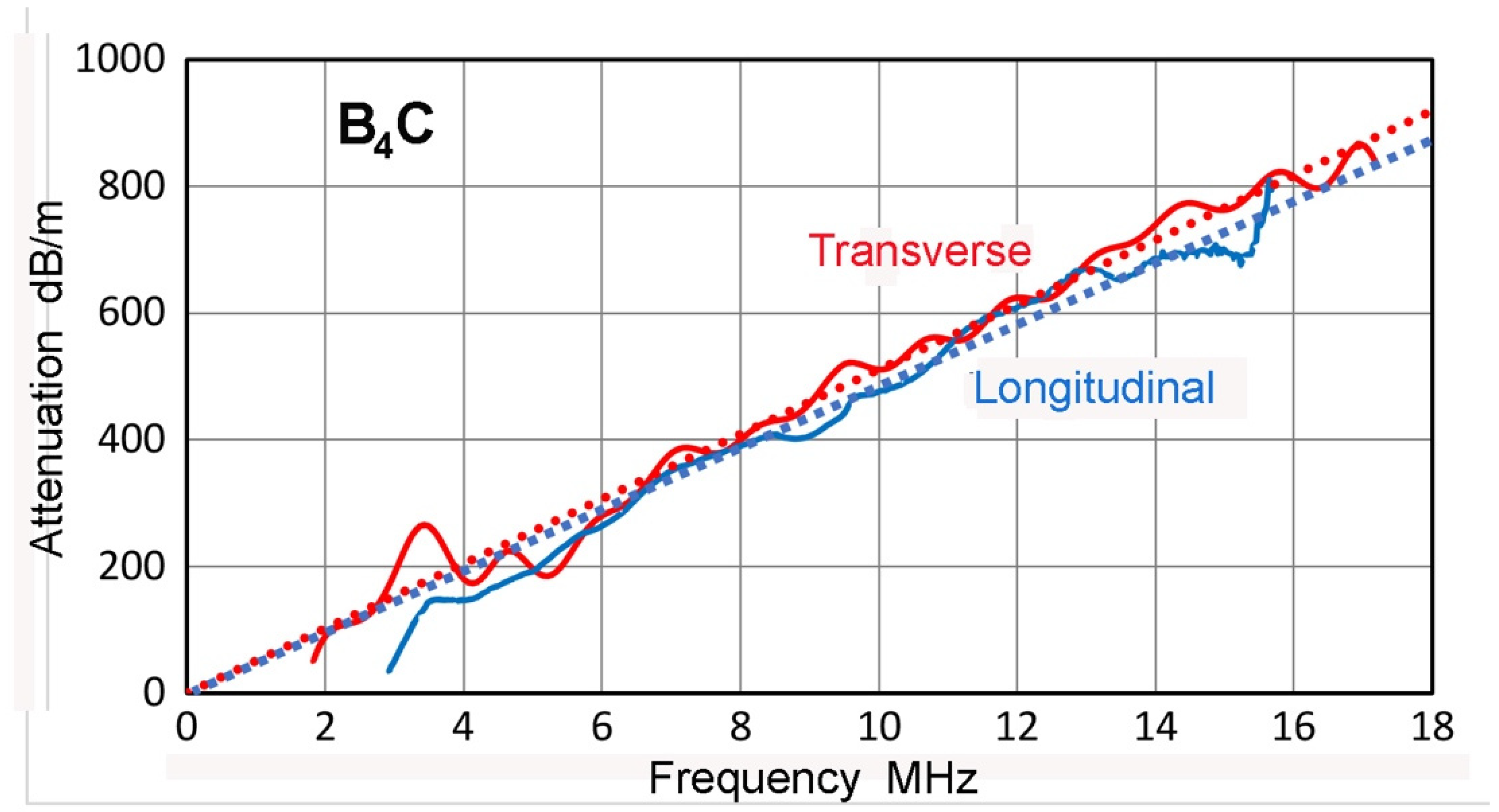
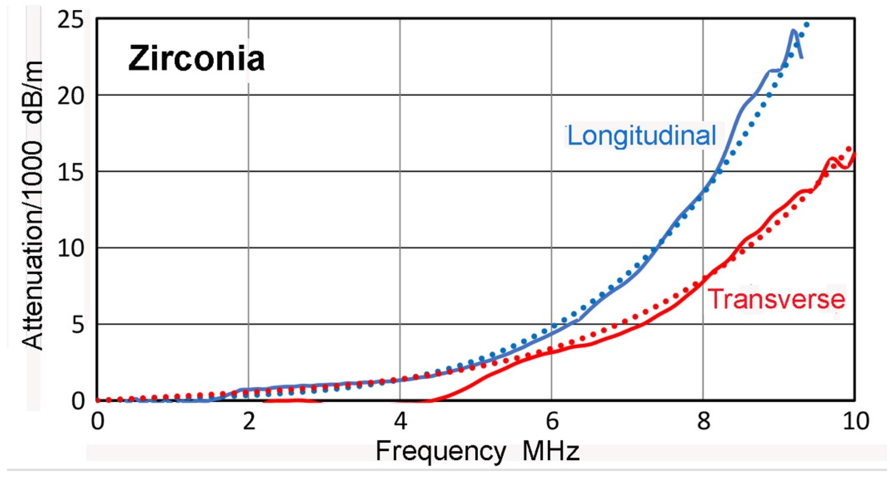
The attenuation coefficients of B4C increased linearly with frequency. Figure 8 illustrates this behavior. Both longitudinal and transverse attenuation exhibited linear dependence with moderate Cd and Cdt values. In this and other figures that follow, solid lines show observed attenuation and dotted lines represent least-square fitted relations. Lines are in blue for longitudinal waves and red for transverse waves. In B4C, the slopes were similar with the transverse attenuation being 11% higher. This is reflected in the listing of Cdt/Cd in Table 3. Damping factors, η (or ηt) calculated from Cd and v (or Cdt and vt) were 0.024 and 0.017, with their ratio, ηt/η, of 0.69. The linear frequency dependence was limited to three other cases of Al2O3, which had Cdt/Cd values of less than unity. That is, longitudinal attenuation is higher than transverse attenuation. All other ceramics in Table 3 followed the Mason-McSkimin equation [50], consisting of the linear and fourth-power frequency relations. Figure 9 illustrates this behavior for yttria-stabilized zirconia. The fourth-power terms were large for both longitudinal and transverse attenuation and their contributions became dominant above 5 MHz. Because CR is about two times larger than CRt, the longitudinal attenuation is higher than transverse attenuation at f > 5 MHz despite having Cdt/Cd of 1.76. When the fourth-power component is ignored, overestimates of Cd and Cdt values occurred. This happened for the case of WC reported in earlier studies [43,44].
Elastic constants obtained in this work are next compared with previously published values, especially with those on single crystals of B4C, YSZ, WC and sapphire (α-Al2O3). Additionally included were those from polycrystalline WC cermet and Si3N4. Results are tabulated in Table 4, listing Young’s modulus, E, shear modulus, G, Poisson’s ratio, ν, C11, C33, C44, C12, C13, Thickness, and Density. Values of E, G and ν calculated from Cij were from the cited references [55,56,57,58,59,60,61,62,63,64,65,66,67]. Agreements between nominally same materials were good; e.g., for B4C and WC cermet. Reductions in E and G (also ν) due to the additions of SiC to Si3N4 were consistent. In terms of Cij values, SiC has higher C11 and C44 than those of Si3N4 (by 25% and 46–65%), while both have similar C33. In yttria-added Si3N4 and Si3N4-20%SiC, Woetting et al. [64] reported an increase in E from 316 to 324 GPa. Thus, the observed softening in Si3N4-SiC in this study needs further evaluation. Some large deviations were found, e.g., YSZ and sapphire. In the case of YSZ, the differences are expected from sample materials since the sample in this work was made in the early days of YSZ development. For the sapphire disc used here was previously assumed to be of R-cut (the second pyramidal plane (102)), but it is closer to the A-cut (with prismatic (100) face).
Among the hard ceramics tested, YSZ showed high attenuation, joining translucent alumina and sapphire with attenuation coefficients exceeding 100 dB/m/MHz. YSZ is expected to have a fine structure, typically with sub-µm grain size (Figure 1 in [65]). However, its density is indicative of approximately 10% porosity. The translucent alumina sample has a low porosity of 2% from its density and a typical microstructure showing low void counts (Figure 10 in [65]). More recent YSZ microstructures contained few voids and larger grain sizes [64]. Such materials will be useful for studying the sources of YSZ attenuation when large enough samples become available. Sapphire has even lower porosity as its density is close to the theoretical density. Yet, all three high-attenuation ceramics have attenuation coefficients nearly twice or more than those of the sintered alumina sample that has a higher porosity of about 16%. This density-based porosity estimate is comparable to 18% porosity, which was obtained by comparing v and vt of alumina ceramics [6]. Thus, the observed high attenuation cannot be attributed to porosity alone. YSZ has a cubic crystal structure, but its anisotropy factor is 0.37, indicating that it is anisotropic [57]. Alumina in this study is α-Al2O3 and hexagonal. When it is approximated using only three of its six stiffness constants, C11, C12 and C44, the anisotropy factor is 0.86. Thus, YSZ is likely to be as anisotropic as alumina. Sapphire is anisotropic with its A-cut surface being the prismatic plane. Since it has no grain boundary, its high attenuation is difficult to explain since its high hardness precludes dislocation motion as the source of damping. This difficulty also extends to YSZ and polycrystalline alumina.
Carbides and nitrides have fine microstructures with typical grain sizes of under 10 µm [55,65,67,68,69,70]. This appears to be the primary reason for their relatively low attenuation since Rayleigh scattering derived by Mason [50] is proportional to the third power of the size of scattering center. Converting Mason’s equation to an attenuation coefficient, α, one obtains
where S is anisotropy-induced scattering power of a grain and Lc is grain diameter. As noted above, dislocation damping is also expected to be low in materials with Vickers hardness exceeding 1000. The WC and Si3N4 samples had Vickers hardness of 1755 (1 kg load) and 1170 (300 g load), while B4C was reported to have 3200 [71] and 1430–2300 for Si3N4 [64,72]. In B4C, sintering and hot pressing slightly decrease carbon content and also leave the intergranular amorphous phase [73]. Its anisotropy factor of 0.80 suggests low attenuation from grain boundaries, even with the presence of the intergranular glassy phase. In fact, attenuation due to Rayleigh scattering was absent, possibly due to the filling of remaining voids.
α = 7.51 × 10⁴ S Lc3 f4/v4,
The tungsten carbide sample is actually a cermet, containing a 16% Co binder. Typical microstructures of WC of the same density as the present test sample consisted of 0.3–5 µm blocky WC grains in the Co matrix [55,65]. The difference of their acoustic impedances is more than a factor of two (ZWC = 98.3 and ZCo = 42.0 Mrayl). Thus, the Co binder phase is expected to scatter propagating waves. However, low Rayleigh scattering effects were observed as listed in Table 3. Attenuation of WC with 16% Co was given as 17.9 dB/m at 10 MHz in [30], which is about 18 times lower than α = 325 dB/m at 10 MHz of Test No. 3 (cf. Table 3). The reported α for WC also had f2.3-dependence [30], giving α of 0.082 dB/m at 1 MHz for WC if the same slope extends downward. The lower α values in WC by the ASTM C1332 method were consistent as in the cases of SiC and Si3N4, discussed in Section 1 [33,34,35,36]. In fact, only a few metallic alloys (Al-2011, Al-2024 and Mg-AZ61) had that level of low attenuation of ~18 dB/m at 10 MHz. Considering the absence of ringing of a hanging WC rod upon hitting, it is difficult to accept attenuation comparable to or lower than that of low-damping Al alloys.
Silicon nitride showed two to three times higher longitudinal attenuation than the two carbides, B4C and WC. On the other hand, transverse attenuation was the lowest among this group of hard ceramics. With the addition of SiC, the longitudinal attenuation coefficient was reduced from 84 to 41 dB/m/MHz, but the transverse attenuation coefficient increased from 2.5 to 18.5 dB/m/MHz. Additionally, Rayleigh scattering effects were higher for Si3N4 and Si3N4 + 10%SiC in transverse mode. SiC additions to Si3N4 have been examined using Xray and microscopic methods [69,74]. Only the two constituents, Si3N4 and SiC, were present in Xray diffraction spectra. Transmission and scanning electron micrographs also showed mixtures of Si3N4 and SiC. These results imply that observed decreases in the density due to SiC additions (3.18 to 3.08 and 2.97 Mg/m3) are caused by additional porosity of 2.1 and 6.6%. The porosity contents correspond to the reduction of the Young’s modulus of Si3N4 by 2.4 and 10.7% when the SiC contribution is ignored. These two sets agree well. However, since the E of SiC is 46% higher than the E of Si3N4 (taken as 344 GPa), E reduction is higher than the effects expected from the porosity. This additional E reduction may arise from low intergranular bonding between Si3N4 and SiC grains. Si3N4 with 20% SiC with Y2O3 showed the fracture toughness of 5.2 MPa·m0.5, which was at 71% of that of Si3N4 [64]. As noted earlier, the 20% SiC addition increased E only slightly. Thus, systematic studies are needed to clarify elastic responses of Si3N4-SiC ceramics since the methods of ceramic consolidation must be taken into account.
The poor intergranular contact and porosity in Si3N4-SiC ceramics are expected to increase attenuation through multiple reflections and scattering. It is possible that frictional loss at the boundaries contribute to ultrasound absorption. While the presence of similar internal nano-scale flaws has not been known at this time, it is plausible in some hard ceramics. In oxide ceramics containing alumina and zirconia, polygonal grain structures have often been observed [65]. However, these showed higher attenuation than carbide ceramics as discussed above. Thus, separate mechanisms for attenuation must be conceived. Presently, no viable physical mechanisms exist for attenuation in ceramics with varied microstructures and intercrystalline bonding conditions. It is also necessary to consider the presence of the glassy phase at the boundaries. In turn, this indicates that the attenuation characteristics can be used to explore the condition of intergranular boundaries.
4.2. Glasses and Common Ceramics
Attenuation coefficients of longitudinal and transverse modes of glasses and common ceramics are covered in this section. Table 5 summarized the results. This group includes four clay ceramics, steatite and porcelain as well as two resin-bonded grinding discs. These eight tests (Test Nos. 9 to 16) were completed including one new sample of steatite and others with improved polishing. Test No. 13 used a reduced thickness sample of previous Test No. C20 for both modes. Other seven test results were previously reported and are shown for comparison. These are comprised of five silicate glasses, Macor glass ceramic, and a ceramic tile listed with the previous test numbers. Material information was mostly unavailable (except for Macor from Corning [43]). Elastic constants obtained are tabulated in Table A1 in Appendix A. Young’s modulus, E, shear modulus, G, Poisson’s ratio, ν, Thickness, and Density are listed. It is noted that Poisson’s ratio was less than 0.3 in all the samples.
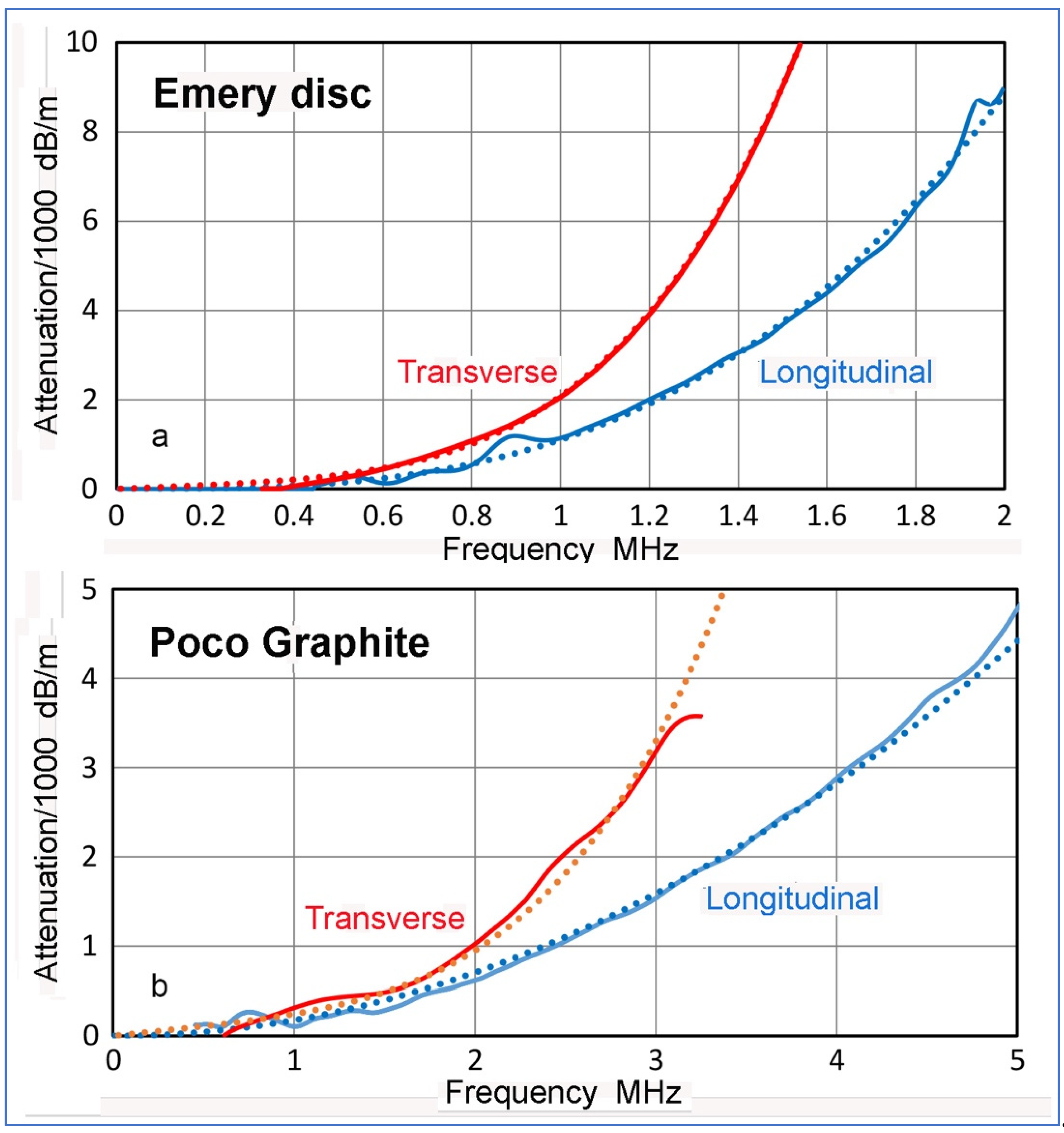
The frequency dependence of attenuation coefficients was primarily linear or with a Rayleigh scattering component of f4-dependence, that is, the Mason-McSkimin relation. A fired clay (Test No. 11) showed f2-dependence for the longitudinal attenuation, while bonded emery (Test No. 10) showed f3-dependent attenuation for the longitudinal mode. In both cases, the attenuation coefficient, Cd, vanished, but high values of C2 and C3 lead to the attenuation coefficients at 1 MHz of 2041 and 1110 dB/m, respectively. Figure 10a shows the longitudinal and transverse attenuation coefficients vs. frequency plots for the bonded emery disc in blue and red curves as before, with solid and dotted curves being observed and fitted data. Here, the blue curves show the frequency-cubed relation, while the red curves represent the Mason-McSkimin relation. Figure 10b illustrates the frequency-squared relation, exhibited by a Poco graphite (Test No. 26) since this sample showed the same a-f2 dependence for both wave modes.
For Tests 9 to 16, all except bonded SiC had higher transverse attenuation than longitudinal attenuation, while silicate glasses showed the reverse behavior (except tempered S-L glass, Test C43). Here, fused silica is excluded from consideration as no attenuation was detectable.
In terms of the levels of attenuation, resin-bonded and porous ceramics (Test Nos. 9 to 13, C21) exceeded 100 dB/m/MHz. Qualitatively, their high attenuation can be attributed to viscoelastic resin or air between ceramic grains, but predictive theories need to come from future efforts. High transverse attenuation of steatite was surprising since its density (ρ = 2.78 Mg/m3) corresponds to 2.5% porosity [75]. This is only slightly higher than the 1.6% found in a steatite sample (ρ = 2.79 Mg/m3) using X-ray microscopy by Perfler et al. [76]. In their work, detailed pore size statistics were obtained, showing the average pore size of 15 µm with a range of 10 to 35 µm. Their E value was at 120 GPa, which was 8% higher than that of Test 15. They showed E decreased with decreasing density, reaching zero E at 50% porosity. This rate of decrease was smaller than in alumina, which reached zero E at 38% porosity with extrapolation. General trends were comparable to others [7]. Both steatite and porcelain had high Cdt/Cd and ηt/η ratios of 2 to 4. These results markedly differed from that of sintered alumina, which yielded low Cdt/Cd and ηt/η ratios of 0.76 and 0.41. The different attenuation responses to longitudinal and transverse waves cannot be explained at present.
4.3. Other Ceramics, Mortars and Composites
Attenuation coefficients of longitudinal and transverse modes of other ceramics, mortars and composites are summarized in Table 6. This group includes mortars, graphite, ferroelectrics, other ceramics and composites. Some samples, such as mortars, graphite and carbon–carbon (C-C) composites, were reduced in thickness in order to obtain transverse attenuation coefficients. Graphite, C–C and SiC–SiC composites needed measurements in two or three directions because of anisotropy. The MnS sample was also ground to improve parallelism. Again, elastic constants obtained are tabulated in Table A2. In several cases of graphite plate and zeolite composite, v and vt were too close, making Poisson’s ratio grossly negative. This resulted in the Young’s modulus lower than the shear moduli. Only the shear moduli are reported for Tests 22, 24 and 27 and marked by *. When Poisson’s ratio was above −0.3, these were included since a negative Poisson’s ratio was a consequence of the presence of certain types of voids [77].
In earlier studies, 50 mm cube mortar samples were used [43]. These were cut to 6.4 to 11.2 mm thickness as listed. The void contents given were measured using a set of cube samples with a water-immersion method given in ASTM C642-21 [78]. Here, void content is used for porosity conforming to ASTM terminology on concrete and mortars. Additional voids in samples of Test No. 18 and 19 were produced by adding an air-entraining agent (see [43] for more details). This entrained type of void in concrete is one of four types [79] and pre-existing void nuclei grew with the agent addition. The void content, V, increased from 10.7% to 13.2 and 17.7%. However, the contents of voids unconnected to the surface, also known as entrapped voids, cannot be detected by the ASTM C642 method. The elastic moduli and mass density data on Table A2 indicate larger changes, contradicting the observed V increases of 2.5 or 7%. When it is assumed that the sample without air-entrainment agent has a 10.7% void (as measured by the immersion method) and using its density of 2.00 Mg/m3, the density of a void-free mortar is 2.24 Mg/m3. Using this value along with the densities of samples of Tests 18 and 19, the latter two have V of 22.8% and 31.3%. These will be used in the following discussion. In addition to the dry condition, the thinned mortar samples were also tested in a water-saturated condition. The samples were immersed in water at 30 °C for 180 h. They were tested within 20 min. after their removal from water and wiped dry, similar to the ASTM-C642 procedure. For the transverse mode testing, it was necessary to use cyanoacrylate glue in lieu of ultrasonic shear gel, which was liquified by saturated water from the mortar sample. The saturated samples (Tests 17a, 18a and 19a) showed approximately 15% higher density, compared to their dry conditions.
Graphite plate appeared to be of common ATJ grade from its density (1.77 Mg/m3), which was the same grade as one used by Papadakis [32]. It was previously measured only in the thickness (or S) direction, but samples were cut into 2.1–3.2 mm thickness in the longitudinal (L) and transverse (T) directions in addition to the S direction (Tests 22–27). Here, S represents short-transverse direction being the surface normal. Estimated porosity of this plate was 22% with respect to the theoretical graphite density of 2.269 Mg/m3. For the Poco graphite rod, the radial and axial directions were distinguished. Tests 33 to 37, C7 and C8 used identical samples as in the previous studies. A pyrolytic graphite plate was tested in the S direction only (Test No. 29). A Gypsum disc was made by mixing calcium sulfate dihydrate (Fix-It-All, Custom Building Products, Santa Fe Springs, CA, USA) with water at a ratio of 1 to 0.43 and molded. Its estimated porosity was 26% in comparison to the theoretical density (2.32 Mg/m3) of calcium sulfate dihydrate (CaH4O6S). Zeolite composites were designed for sound absorbing applications and contained 46–60% zeolite, 30% polyurethane and 10–24% isocyanate by weight (Galadari, M., private communication). These are designated as Zeolite composite 1 to 3, with the density changing from 1.11 to 0.90 Mg/m3. That is, porosity increased by 18% as density decreased.
C-C composite was a brake disc of 424 mm outside diameter, 272 mm inside diameter and 10.4 mm thickness. Manufacturer’s information is unavailable. It was reinforced using carbon fiber tows in three dimensions along the radial (R), circumferential (C) and thickness (S) directions. Comparing its density to the theoretical value of 2.269 Mg/m3, the porosity is estimated to be 15.6%. Thin samples were prepared with surface normal in these three directions. For the R and C directions, two plates were aligned and glued. The SiC-SiC composite sample had nominally [±45°]6 fiber reinforcement, but fiber alignments were poor. Its surfaces were ground using a diamond disc.
Attenuation coefficients of longitudinal mode of mortar samples in dry and saturated conditions can be fitted to the linear plus frequency-cubed dependence. Transverse attenuation coefficients in both conditions followed the Mason-McSkimin relation or the linear plus fourth-power frequency dependence. Regardless of the frequency dependence type, attenuation coefficients were large and also increased with the void contents, except for the longitudinal attenuation in the saturated condition. Both Cd and damping factors were especially high for dry samples with void additions (Tests 18 and 19) in the longitudinal mode. In comparison, transverse attenuation was less affected by the presence of the additional void. This behavior in the dry state is reflected in sharp decreases in Cdt/Cd and in ηt/η. In the saturated condition, the values increased. As is well-known [8,80], the longitudinal and transverse wave velocities of the mortar samples decreased as the void content increased. Relative velocity reduction due to void was comparable between longitudinal and transverse waves. These changes affected the elastic moduli, as tabulated in Table A2. Young’s modulus decreased by 40 and 64% and the shear modulus similarly dropped. These changes were much higher than the density reductions. This effect on elastic moduli has been studied extensively as summarized in a review [75]. Early studies also established that increased void contents cause higher attenuation (or lower Q values) in rocks [81,82].
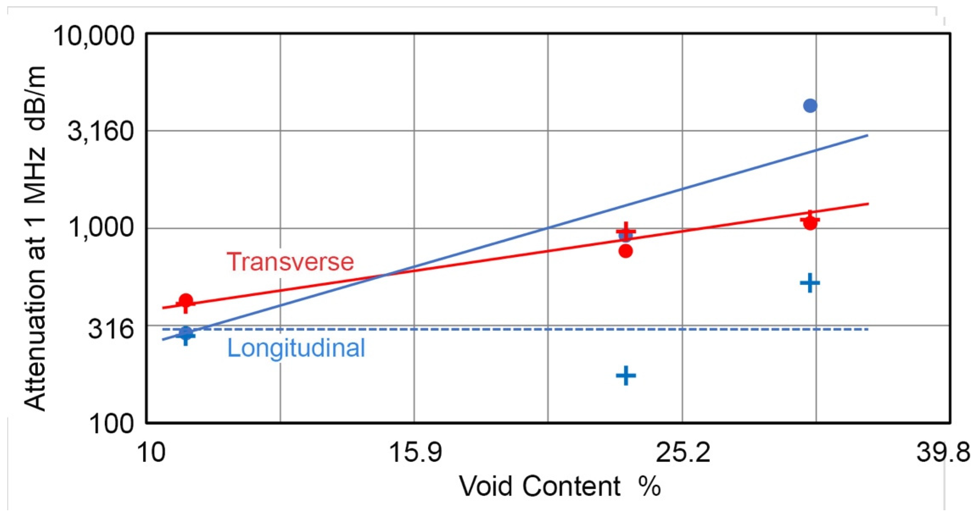
In order to examine the void effects, the attenuation coefficients of the mortar samples at 1 MHz, the α1M and αt1M were obtained by using Cd + C2 and C3 for the longitudinal mode and Cdt + CRt for the transverse mode. Results are plotted with blue dots and + symbols for α1M and red dots and + symbols for the αt1M against the void content on a log–log scale in Figure 11. Here, the + symbols are used for the saturated conditions. As discussed above, the sample without air-entrainment agent has a 10.7% void (as measured by the immersion method) and the samples of Test No. 18 and 19 have a V of 22.8% and 31.3%. While the data is limited, it appears that α1M in the dry condition increases with the second power of %void, V2, and the αt1M shows a linear relation, αt1M V. Blue and red lines represent these relations, while the blue dashed line is for the α1M of the saturated samples. A theoretical prediction of attenuation based on the scattering from spherical voids was given [83,84] as
where A is a constant inclusive of the elastic constants and wave velocities and r is the void radius. The αt1M -V relation and the f4-dependence for the transverse attenuation agree with Rayleigh theory, Equation (15), but the α1M-V2 relation and f2- or f3-dependence for the longitudinal attenuation have no theoretical basis at this time. The reduced effect of voids on α1M in the saturated state indicated that the longitudinal waves have less mismatch in the acoustic impedance since Z within the void increases from nil to 1.5 Mrayl of water. Z for the mortar sample ranges from 3.5 to 7.3. For the transverse waves, αt1M values were unaffected since both air and water cannot support this wave mode. This absence of water-saturation effect on the transverse attenuation appears to be unreported previously and should be confirmed by additional studies.
α = Ar3f4 V,
The presence of the void affected the elastic moduli strongly, reducing E and G to 30–40% of the initial values of the sample. It is common to the behavior of hard ceramics as documented for alumina [6] and was confirmed in a recent data compilation on pervious concrete [85]. It is interesting to note that the void content of 23 to 31% is called optimum for pervious concrete [86], while it is less than 14% for normal concrete [79,80]. When the sample thickness was reduced, E and G values increased by 3 to 7%, indicating that microstructural variation occurs within even a small-sized mortar sample, similar to the variation known for larger concrete [87]. This apparently caused large reduction in attenuation found in this study compared to the previous reports that used 50 mm cubes [43,44].
The saturation of entrained voids also increased wave velocities, producing increases in E and G values (cf. Table A2). From the corresponding dry states, E values increased by 41 to 50% and G values by 49 to 68%. The study of acoustic wave propagation in media with voids and cracks filled with liquid has been an important and active field, based on the Biot theory [88,89,90]. The applications of the Biot theory to seismic exploration have yielded broad successes [89], but its extension to the ultrasonic frequency range has remained static. The Biot approach introduced damping terms into the elastic constant operators [88], but their interpretation in terms of void and liquid characteristics has not been developed. At higher frequencies, fluid flow within voids [90] can hardly be a factor in wave attenuation. Increases in the longitudinal wave velocity of concrete due to water saturation was reported in 1980 [91], continuing to the present [92]. However, no comparable studies on attenuation have been made.
The observed increases in the longitudinal wave velocity (by 4.5 to 11.5%) and E (by 41 to 50%) from water-filled voids are consistent with the replacement of air with water, having 21.8-times higher bulk modulus than that of air. The observed increases in the transverse wave velocity and G from water-filled voids were 14.2 to 20% and 49 to 60%, respectively. It is difficult to attribute these increases to water-to-air replacement as both cannot support transverse waves. These changes and the absence of saturation effects on transverse attenuation require further study since no conceivable mechanisms can be suggested at this stage.
Velocity and attenuation data for graphite plate samples (Test 20 to 25) showed orthotropic behavior. This is most clearly found in the Young’s moduli of the three directions; 14.7–15.2 GPa for the L direction and 7.8 or 7.6 GPa for the T or S direction (cf. Table A2). The longitudinal attenuation data showed the frequency-squared dependence (cf. Table 6) and C2 values increased from L to S to T directions. However, the damping factor, η, was the highest for the L direction because of the higher velocity. For the transverse attenuation data, the frequency-squared dependence was again found for all the tests However, a clear trend on the directional effects was difficult to recognize and the damping factor, ηt, was within the range of 0.073 to 0.13. Comparing its density to the theoretical value of 2.269 Mg/m3, the porosity of this graphite plate was estimated as 21.5%. This contributed to its high attenuation together with its coarse grain microstructures. The values of α in this study were two to three times higher than those of Papadakis [32], who reported 348 to 522 dB/m at 1 MHz using the buffer-rod method.
The Poco graphite rod (Tests 26 to 28) showed lower attenuation than the ATJ graphite plate above, reflecting its more homogeneous and fine-grained microstructure, even though the density is slightly less than the plate sample (cf. Table 6). All the Poco graphite samples showed the frequency-squared relations (cf. Figure 10b). In the axial direction, η and ηt were nearly five and three times smaller than those of the ATJ graphite plate. Differences with the plate data were less in the radial direction for both longitudinal and transverse attenuation. The elastic moduli were not expected to be isotropic, and were found to be transversely isotropic because of an extrusion process during its manufacturing. The transverse propagation behavior in the radial direction with polarization along the axial direction showed an abnormal Poisson’s ratio, leaving the Young’s modulus undetermined. Changing from the axial to radial direction, both E and G values decreased by approximately a factor of two (cf. Tests 26 and 28 in Table A2). A pyrolytic graphite plate of the density nearly identical to that of Poco graphite showed similar attenuation behavior in the S direction to that of Poco graphite in the radial direction.
Test No. 30 to 32 examined ferrites and Fe-Nd-B magnet. Ferrites showed moderate attenuation, falling between ceramic tile and porcelain (Test No. 14 and 16). Fe-Nd-B magnet with the remanance of 0.45T showed seven-times more attenuation than the ferrites. This high attenuation appears to be from the use of resin bonding as were the cases for Test No. 9 and 10 [93]. Sintered Fe-Nd-B magnets are expected to show lower attenuation similar to the ferrite magnets (Tests 30 and 31). MnS (Test 33) was hot pressed and ZnSe (Test 34) was made by chemical vapor deposition (CVD). Both showed moderate attenuation similar to hard ceramics, reflecting their uniform and fine-grained microstructures. Additionally, these two had higher transverse attenuation than longitudinal attenuation. Two ferroelectric ceramics of lead-zirconate titanate (PZT-5A, polarized in the thickness direction) and barium titanate (BaTiO3) were previously examined (Tests C7 and C8). Their attenuation behavior was close to that of Fe-Nd-B magnet. Evans et al. [33] obtained attenuation for a PZT of 250 dB/m at 5 MHz using the buffer-rod method, which was five-times smaller. A part of the larger attenuation of the C7 sample was due to its 3% porosity, calculated by using the theoretical density given in [41]. These all showed the linear frequency dependence, similar to the result of [38].
Tests 33 to 36 are on sound absorbing materials of gypsum and zeolite composites. Gypsum had about twice higher Cd and Cdt values of mortar sample (Test 17), but showed less attenuation than mortars with voids (Tests 18 and 19). Zeolite composites had the highest attenuation among inorganic materials tested in this study, although their attenuation was less than some wood and lumber samples [43]. Cd and Cdt values of the zeolite composites ranged from 2385 to 5940 dB/m/MHz. Cdt values were larger than the corresponding Cd values (cf. Tests 36 and 38 in Table 6). E and G values were below 10 GPa, decreasing with increasing porosity (cf. Table A2). Test 38 showed a negative Poisson’s ratio as vt was equal to 0.745 v, reflecting a high porosity of more than 18%. Note that void geometry is a critical factor for the observation of negative Poisson’s ratio [77]. In alumina, for example, 25% porosity reduced its Poisson’s ratio from 0.250 to 0.193 [6].
A carbon–carbon (C-C) composite disc was tested next and the results are given as Tests 39 to 44. Because of its tri-directional carbon-fiber reinforcement, six tests were conducted, similar to those of ATJ graphite testing discussed above. The directions of wave propagation are denoted as S, R and C, as noted above. The directions of polarization for transverse attenuation tests were two remaining directions. As expected from the reinforcement structure, the longitudinal wave velocity exhibited orthogonal behavior with 14.4, 11.7 and 13.1 mm/µs for the S, R and C directions, while the transverse wave velocity showed nearly isotropic behavior, within the range of 2.19 to 2.89 mm/µs. In the latter, the maximum and minimum velocities were found in the R direction. The linear frequency dependence of attenuation prevailed in all 12 tests. Longitudinal attenuation coefficients varied from 535 (C direction) to 1941 (R direction) dB/m/MHz and transverse attenuation coefficients from 846 (C direction) to 2783 (R direction) dB/m/MHz. The transverse attenuation coefficients were always higher than the longitudinal coefficients. Indeed, this C-C composite showed the orthotropic attenuation. The levels of attenuation were high and only exceeded by those found in mortar with the highest porosity and zeolite composites. While the fiber reinforcement and the matrix are both carbonaceous, the fibers have a highly oriented molecular arrangements with high elastic moduli along the fiber direction. The matrix, on the other hand, is based on tar impregnation and subsequent carbonization, making it nearly isotropic. Thus, acoustic impedance mismatch between the matrix and fibers is expected, contributing to wave attenuation. Estimated porosity of 15.6% also added attenuation. For both types of attenuation, distributions of fibers, matrix and voids dictate how waves propagate and attenuate. At this stage, no detailed study of such a structure is available in the open literature.
An SiC-SiC composite plate was tested in the thickness direction only, because of the sample size available. Attenuation showed the Mason-McSkimin behavior for both longitudinal and transverse waves. Cd and Cdt values were high, at 793 and 778 or 1479 dB/m/MHz, respectively. From the measured density, porosity was estimated to be 23.5%. Again, the fiber and matrix are expected to have an acoustic impedance mismatch. These are expected to cause high attenuation in this composite.
This group showed a wide range of attenuation behavior from the low side of CVD ZnSe and sintered ferrites to the high side of mortars, zeolite composites and C-C composites, which have high porosity. Elastic moduli summarized in Table A2 contained several samples with abnormal Poisson’s ratio because of high ratios of vt and v, or vt/v. Under the isotropic elasticity condition, Poisson’s ratio becomes negative when vt/v value exceeds √2/2 = 0.7071.
4.4. Rocks and Single Crystals
Attenuation coefficients of longitudinal and transverse modes of rocks and single crystals were next determined. See Table 7, Tests 47 to 56. Most samples were evaluated previously for at least the longitudinal attenuation, but sample thicknesses were reduced and retested. Tektite sample (Test 54) was newly added. Results of Tests C38 to C50 are listed for comparison. The linear or Mason-McSkimin relations were observed for most, except granite and marble, which had the frequency-squared relations (Tests 55 and 56). Cd and Cdt values ranged from low to high, with ADP and Si single crystals (SX) at nil or low attenuation and travertine and granite showing high values. The majority exhibited moderate levels of attenuation. Table A3 listed the elastic constants based on the wave velocity data. Soga and Anderson [20] previously measured the elastic constants of tektite and the present values matched them within 2%.
Pyrophyllite sample was hardened by heating it at 900 °C for 1 h. After the firing, Cd was reduced by a third, but Cdt was down by only 15%. The firing converts pyrophyllite to pyrophyllite dihydroxylate, modifying the Al-O bond configuration. This apparently caused changes in the attenuation behavior. Relatively high Cd value of tektite is surprising as it is glassy, but its lower Cdt value is of the same trend as silicate glasses, listed in Table 5.
Travertine (Test 53) showed the highest Cd and Cdt values in this group. It has many visible cavities and its density indicates 11% porosity in the matrix in comparison to the density of calcium carbonate (2.71 Mg/m3). Structural defects other than void appear to add attenuation, although microstructural analysis could not be conducted in this study.
Granite (Test 55) was retested using a sample with its thickness reduced by 81.7%. As the high frequency component was enhanced, the frequency-squared dependence emerged in the longitudinal mode, extending to 3.4 MHz. The previous spectrum (Test C33) can also be fitted to the same f2-dependence to 1.3 MHz upon re-analysis, but its C2 coefficient was higher by a factor of 2.2. That is, the longitudinal attenuation was reduced by about a half using the thinner sample. (Actually, the thin sample was cut from one side; i.e., it is normal to the thickness direction previously used. Thus, directional effect may be present.) In contrast, the linear part of its transverse attenuation was 1.22× higher from the thickness reduction and the f4-term emerged over 1 to 2 MHz segment. The η and ηt values in this work were 0.0905 and 0.135. These are close to those reported recently for an Australian granite of 0.0707 and 0.0819 [94]. Both η values are several times larger than those measured at MHz frequencies, which were cited in Knopoff’s classical review [13]. Sample thickness reduction affected the longitudinal attenuation of marble slightly (or 22% higher), but the transverse attenuation was nearly doubled in terms of ηt value. The cause for the effects on the transverse mode is uncertain at present.
Comprehensive collections of the elastic and anelastic properties of rocks can be found in [15,16]. The wave velocities are tabulated for more than 30 minerals along with the densities and Poisson’s ratios. Results of the present study generally matched with those listed. Schön [15] plotted the longitudinal attenuation of seven types of minerals against frequency from 10 Hz to 10 MHz, using data from the literature. This attenuation was due to absorption, or the hysteretic component. Linear frequency dependence was found for metamorphic rocks, consolidated sediments, magnetic rocks, limestones and dry sands. Low consolidated or unconsolidated sediments showed f1.5-dependence. The result showing the dominance of the linear frequency dependence validated the use of frequency-independent damping factor, η (or Q−1) for rocks and minerals. The constancy of Q−1 (preferred term in geoscience) at f below 1 MHz has withstood the test of time since the early days [13,95], but additional scattering terms are needed as shown in this study at higher frequencies. The attenuation of granite (Test 55) was within the range of metamorphic rocks (80 to 450 dB/m at 1 MHz), while that of marble (Test 56) was 40% lower. Since both showed the frequency-squared relation, marble’s attenuation matched at 2 MHz, while that of granite moved higher. In the case of travertine (a terrestrial limestone), α1M of Test 53 was 15 times higher than the corresponding value for limestones (measured at f = 5.8 MHz) in [15,16]. This appears to arise from higher porosity. A note of caution is needed here as some attenuation studies in geoscience skipped the correction needed for diffraction losses e.g., [94,96]. This omission has been justified by making substitutional measurements in a standard sample of the same shape, typically using aluminum, assumed to have a high Q value of 150,000 [71,72,94]. However, no aluminum alloy possesses MHz-attenuation lower than fused silica [43] and the diffraction loss can be severe below a few MHz. For example, Wanniarachchi et al. [94] used a pair of 5 mm diameter transducers (presumed to have a 4 mm diameter piezoelectric element), causing 35 to 21 dB loss at 0.2 to 1 MHz at 76 mm distance. Since they used 38 mm diameter samples, sidewall reflections were dominant in a replication test. Unless only the direct signals were analyzed, their attenuation data contained incorrect propagation distances. In earlier studies on rocks [76,77], attenuation results were fitted to α’ vs. f relations, but observed data showed non-zero vertical intercepts. That is, arbitrary shifts in observed attenuation levels were applied. Thus, such data sets need further analysis. Additionally, in the geoscience field, there exists efforts to account for multiple sources of attenuation, such as cracks and porosity, e.g., [97]. However, the use of standard linear solids without considering physical mechanisms resulted in damping peaks at 0.1 to 1 MHz. No such peaking behaviors are known, and other approaches need to be explored.
Finally, Table A4 listed the elastic constants of various mineral samples that were smaller than the size needed for attenuation measurements. This group includes two carbides, Fe3C7 and Cr3C7, produced by high-pressure syntheses at 1300 °C under 4 GPa (Hirano, S., Nagoya University, Nagoya, Japan), actinolite, jadeite and nephrite samples (Gaal, R., Gemological Institute of America, Santa Monica, CA, USA), Santa Monica slate (outcrop, Encino, CA, USA), Mono Lake obsidian (Lee Vining, CA, USA) and a hematite single crystal. Note that a pair of near-square faces of hematite, <100> in the pseudo-cubic notation, were used for the velocity determination. The obsidian sample showed a low Poisson’s ratio even though its density and E value were similar to most silicate glasses. It has G = 37.7 GPa, which was 23% higher than that of the S-L glass (Test C43).
This section covered a limited range of materials, intended to compliment available elasticity data in the literature, e.g., [15,16]. While E and longitudinal velocity (v) values are usually available, G and transverse velocity (vt) values are more limited. Some minerals, such as jadeite, have been studied extensively in connection to seismic anisotropy e.g., [98]. On the other hand, attenuation data is rarely available, especially in the transverse mode.
5. Summary
This report provides the attenuation coefficients of ceramic and inorganic materials, covering 74 samples. After experimental reevaluation, the buffer-rod method (including the ASTM C1332 procedures) was found to be impractical since attenuation results were found to be inconsistent due to nonpredictable reflection coefficients. Resonant ultrasound spectroscopy was also shown to be inappropriate for NDE use because of restrictive sample requirements and the lack of transverse-wave capability. Its attenuation data is likely to contain the effects of transverse modes, requiring further study. In this study, attenuation measurements were conducted at ultrasonic frequencies of 0.5 to 16 MHz using through-transmission techniques with diffraction loss correction. The longitudinal and transverse wave modes were tested separately. Elastic constants of tested materials were also given, including additional samples too small for attenuation tests. The levels of attenuation were comparable when previous data were available. Attenuation exhibited four types of frequency (f) dependence, i.e., linear, linear plus f4 (called a Mason-McSkimin relation), f2 and f3. The first two types were most often observed. The obtained results were discussed in terms of available theories in limited instances, since material characterization was inadequate, leaving many aspects of experimental findings unexplained. However, the observed levels of attenuation coefficients will facilitate optimal test design for ultrasonic nondestructive evaluation, which was the primary objective of this study. This study also revealed a wide range of attenuation behaviors, indicating that attenuation parameter can aid in clarifying the condition of intergranular boundaries in combination with imaging studies.
Funding
This research received no external funding.
Institutional Review Board Statement
Not applicable.
Informed Consent Statement
Not applicable.
Data Availability Statement
Not applicable.
Acknowledgments
The author is grateful to E. Bescher, O. Fukunaga, R. Gaal, M. Galadari, S. Hirano, S. Saito, G. Sines and J.M. Yang for supplying some of the samples used in this study.
Conflicts of Interest
The authors declare no conflict of interest.
Appendix A
This part provides additional data on elastic constants in four tables. Listings are similar to Table 5.

Table A1.
Elastic constants of glasses and common ceramics.
| Number | Material | E | G | ν | Density | Notes |
|---|---|---|---|---|---|---|
| GPa | GPa | Mg/m3 | ||||
| 9 | Bonded SiC | 63.4 | 25.3 | 0.259 | 2.32 | This study |
| 10 | Bonded Emery | 10.6 | 4.38 | 0.206 | 2.63 | This study |
| 11 | Fired clay (red brick) | 9.10 | 3.73 | 0.220 | 1.93 | This study |
| 12 | Fired clay (red planter) | 17.5 | 8.20 | 0.068 | 2.18 | This study |
| 13 | Clay ceramic (planter) | 43.1 | 17.6 | 0.225 | 2.18 | This study |
| 14 | Clay ceramic (tile) | 64.4 | 27.9 | 0.155 | 2.34 | This study |
| 15 | Steatite | 111.1 | 45.4 | 0.225 | 2.78 | This study |
| 16 | Porcelain | 110.3 | 47.1 | 0.172 | 2.63 | This study |
| C15 | BK7 glass | 73.5 | 30.1 | 0.224 | 2.51 | [44] |
| C21 | Clay ceramic (tile) | 31.2 | 12.0 | 0.297 | 1.97 | [44] |
| C29 | Macor | 60.1 | 24.2 | 0.240 | 2.52 | [44] |
| C42 | Pyrex glass | 61.8 | 25.9 | 0.191 | 2.23 | [44] |
| C43 | Soda-lime (S-L) glass | 74.3 | 30.4 | 0.223 | 2.48 | [44] |
| C44 | S-L glass, tempered | 74.4 | 30.3 | 0.226 | 2.52 | [44] |
| C45 | Fused silica | 70.7 | 30.3 | 0.167 | 2.20 | [44] |
Table A2.
Elastic moduli of other ceramics, mortars and composites.
| Test. | Material | Density | E | G | ν | Notes |
|---|---|---|---|---|---|---|
| No | Mg/m3 | GPa | GPa | |||
| 17 | Mortar 10.7% void | 2.00 | 24.18 | 10.22 | 0.184 | Dry |
| 17a | Mortar 10.7% void | 2.00 | 34.24 | 15.18 | 0.128 | Saturated |
| 18 | Mortar 22.8% void | 1.73 | 14.72 | 5.99 | 0.230 | Dry |
| 18 | Mortar 22.8% void | 1.73 | 20.74 | 9.28 | 0.117 | Saturated |
| 19 | Mortar 31.7% void | 1.54 | 8.81 | 3.94 | 0.117 | Dry |
| 19 | Mortar 31.7% void | 1.54 | 13.22 | 6.64 | −0.004 | Saturated |
| 20 | Graphite plate | 1.77 | 15.20 | 6.19 | 0.228 | L; pol//T |
| 21 | Graphite plate | 1.77 | 14.65 | 5.86 | 0.249 | L; pol//S |
| 22 | Graphite plate | 1.77 | * | 5.67 | * | T; pol//L |
| 23 | Graphite plate | 1.77 | 7.81 | 4.20 | −0.070 | T; pol//S |
| 24 | Graphite plate | 1.77 | * | 7.37 | * | S; pol//L |
| 25 | Graphite plate | 1.77 | 7.63 | 5.18 | −0.263 | S; pol//T |
| 26 | Poco graphite rod | 1.71 | 16.17 | 6.50 | 0.271 | axial |
| 27 | Poco graphite rod | 1.71 | * | 5.24 | * | radial //axial |
| 28 | Poco graphite rod | 1.71 | 7.08 | 2.98 | 0.188 | radial //circ. |
| 29 | Pyrolytic graphite | 1.72 | 7.85 | 3.37 | 0.165 | S |
| 30 | Ferrite (hard magnet) | 4.99 | 163.94 | 64.31 | 0.275 | |
| 31 | Ferrite (hard magnet) | 5.05 | 169.30 | 66.18 | 0.279 | |
| 32 | Fe Nd-B magnet | 7.50 | 170.26 | 62.21 | 0.368 | |
| 33 | MnS | 3.84 | 68.22 | 27.37 | 0.246 | |
| 34 | ZnSe | 5.24 | 76.57 | 29.43 | 0.301 | |
| 35 | Gypsum | 1.39 | 8.74 | 4.26 | 0.027 | |
| 36 | Zeolite composite 1 | 1.11 | 5.14 | 2.37 | 0.086 | |
| 37 | Zeolite composite 2 | 1.07 | 4.78 | 2.28 | 0.049 | |
| 38 | Zeolite composite 3 | 0.90 | 3.47 | 1.97 | −0.119 | |
| 39 | C-C composite | 1.92 | 33.68 | 11.34 | 0.485 | S, pol//R |
| 40 | C-C composite | 1.92 | 33.68 | 11.34 | 0.485 | S, pol//C |
| 41 | C-C composite | 1.92 | 27.29 | 9.21 | 0.482 | R, pol//S |
| 42 | C-C composite | 1.92 | 47.07 | 16.04 | 0.468 | R, pol//C |
| 43 | C-C composite | 1.92 | 36.68 | 12.39 | 0.480 | C, pol//S |
| 44 | C-C composite | 1.92 | 34.99 | 11.81 | 0.481 | C, pol//R |
| 45 | SiC-SiC composite | 2.46 | 174.81 | 68.84 | 0.270 | S, pol//L |
| 46 | SiC-SiC composite | 2.46 | 208.19 | 91.24 | 0.141 | S, pol//T |
| C7 | PZT-5A | 7.78 | 64.85 | 23.02 | 0.409 | [44], pol#//L |
| C8 | BaTiO3 | 5.70 | 185.63 | 73.87 | 0.256 | [44] |
* Negative Poisson’s ratio omitted. pol: polarization direction, pol#: piezoelectric polarization.
Table A3.
Elastic constants of rocks and single crystals.
| Test. | Material | Density | E | G | ν | Notes |
|---|---|---|---|---|---|---|
| No | Mg/m3 | GPa | GPa | |||
| 47 | Pyrophyllite | 2.68 | 26.84 | 15.83 | −0.152 | |
| 48 | Pyrophyllite | 2.68 | 20.61 | 13.21 | −0.220 | fired |
| 49 | Salammoniac | 1.54 | 25.50 | 12.60 | 0.012 | |
| 50 | Agate | 2.57 | 83.94 | 36.53 | 0.149 | |
| 51 | Malachite | 3.80 | 46.35 | 19.07 | 0.216 | |
| 52 | Soapstone | 2.80 | 62.74 | 25.88 | 0.212 | |
| 53 | Travertine | 2.42 | 61.21 | 24.01 | 0.274 | |
| 54 | Tektite | 2.39 | 78.61 | 32.72 | 0.201 | |
| 55 | Granite (Santa Cecilia) | 2.74 | 64.70 | 24.33 | 0.330 | |
| 56 | Marble (Carrara) | 2.83 | 79.55 | 32.33 | 0.230 | |
| C50 | Rock salt | 2.18 | 38.85 | 15.77 | 0.231 | [44] |
| C38 | Fluorite <111> | 3.13 | 117.32 | 49.58 | 0.183 | [44] |
| C39 | Calcite [001][110] | 2.72 | 57.07 | 20.12 | 0.418 | [44] yellow |
| C47 | Calcite [001][110] | 2.71 | 56.36 | 19.90 | 0.416 | [44] clear |
| C40 | ADP H6NO4P <100> | 1.80 | 24.87 | 8.71 | 0.427 | [44] pol//<001> |
| C40a | ADP H6NO4P <100> | 1.80 | 60.91 | 25.18 | 0.210 | [44] pol//<010> |
| C48 | Quartz SiO2 SX | 2.56 | 69.06 | 27.54 | 0.254 | [44] pol//Z |
| C49 | Si SX | 2.33 | 155.09 | 60.60 | 0.280 | [44] |
Table A4.
Elastic constants of various minerals with longitudinal and transverse wave velocities.
| Test | Material | Density | E | G | ν | v | vt | Thickness | Notes |
|---|---|---|---|---|---|---|---|---|---|
| No | Mg/m3 | GPa | GPa | mm/µs | mm/µs | mm | |||
| 57 | Fe3C7 | 8.61 | 156.90 | 59.07 | 0.33 | 5.18 | 2.62 | 0.83 | Synthesized # |
| 58 | Cr3C7 | 7.22 | 218.26 | 93.57 | 0.17 | 5.69 | 3.60 | 2.64 | Synthesized # |
| 59 | Actinolite | 3.73 | 131.64 | 59.08 | 0.11 | 6.03 | 3.98 | 2.71 | Cat’s eye |
| 60 | Jadeite 1 | 3.30 | 183.71 | 73.21 | 0.25 | 8.21 | 4.71 | 2.86 | Burma |
| 61 | Jadeite 2 | 3.30 | 187.33 | 73.83 | 0.27 | 8.41 | 4.73 | 2.69 | Burma |
| 62 | Nephrite 1 | 2.96 | 113.51 | 45.48 | 0.25 | 6.77 | 3.92 | 2.34 | |
| 63 | Nephrite 2 | 2.96 | 120.59 | 49.76 | 0.21 | 6.78 | 4.10 | 3.99 | AK, USA |
| 64 | Nephrite 3 | 2.96 | 120.40 | 50.00 | 0.20 | 6.74 | 4.11 | 2.26 | New Zealand |
| 65 | Santa Monica slate | 2.63 | 74.85 | 30.05 | 0.25 | 5.82 | 3.38 | 13.3 | CA, USA |
| 66 | Mono Lake obsidian | 2.52 | 79.42 | 37.74 | 0.05 | 5.63 | 3.87 | 6.40 | CA, USA |
| 67 | Hematite, SX | 5.25 | 225.56 | 86.54 | 0.30 | 7.64 | 4.06 | 8.10 | <100> * |
# Synthesized at 4 GPa, 1300 °C. SX: single crystal. * Pseudo-cubic notation.
References
- Krautkramer, J.; Krautkramer, H. Ultrasonic Testing of Materials, 4th ed.; Springer: Berlin/Heidelberg, Germany, 1990; p. 677. [Google Scholar]
- Kishoni, D.; Workman, G.L.; Moore, P.O. Ultrasonic Testing. In Nondestructive Testing Handbook, 3rd ed.; American Society for Nondestructive Testing: Columbus, OH, USA, 2007; Volume 7, p. 600. ISBN 978-1-57117-105-4. [Google Scholar]
- Whitehurst, E.A. The Soniscope—A Device for Field Testing of Concrete. In Proceedings of the 37th Purdue Road School, Purdue University, West Lafayette, IN, USA, 1951; pp. 105–115. Available online: https://docs.lib.purdue.edu/cgi/viewcontent.cgi?article=3009&context=roadschool (accessed on 22 September 2022).
- Firestone, F.A. Flaw Detecting Device and Measuring Instrument. U.S. Patent 2,280,226A, 21 April 1942. [Google Scholar]
- Kim, G.; Loreto, G.; Kim, J.-Y.; Kurtis, K.E.; Wall, J.J.; Jacobs, L.J. In situ nonlinear ultrasonic technique for monitoring mi-crocracking in concrete subjected to creep and cyclic loading. Ultrasonics 2018, 88, 64–71. [Google Scholar] [CrossRef] [PubMed]
- Chang, L.-S.; Chuang, T.-H.; Wei, W. Characterization of alumina ceramics by ultrasonic testing. Mater. Charact. 2000, 45, 221–226. [Google Scholar] [CrossRef]
- Choren, J.A.; Heinrich, S.M.; Silver-Thorn, M.B. Young’s modulus and volume porosity relationships for additive manufacturing applications. J. Mater. Sci. 2013, 48, 5103–5112. [Google Scholar] [CrossRef]
- Ohtsu, M. Acoustic Emission (AE) and Related Non-Destructive evaluation (NDE) Techniques in the Fracture Mechanics of Concrete: Fundamentals and Applications; Elsevier: Amsterdam, The Netherlands, 2015; p. 291. [Google Scholar]
- Godin, N.; Reynaud, P.; R′Mili, M.; Fantozzi, G. Identification of a Critical Time with Acoustic Emission Monitoring during Static Fatigue Tests on Ceramic Matrix Composites: Towards Lifetime Prediction. Appl. Sci. 2016, 6, 43. [Google Scholar] [CrossRef] [Green Version]
- Mason, W.P. Physical Acoustics and the Properties of Solids. J. Acoust. Soc. Am. 1958, 28, 402. [Google Scholar]
- Bhatia, A.B. Ultrasonic Absorption, An Introduction to the Theory of Sound Absorption and Dispersion in Gases, Liquids and Solids; Clarendon Press: Oxford, UK, 1967; p. 427. [Google Scholar]
- Nowick, A.S.; Berry, B.S. Anelastic Relaxation in Crystalline Solids; Academic Press: New York, NY, USA, 1972; p. 694. [Google Scholar]
- Knopoff, L. Attenuation of Elastic Waves in the Earth. In Physical Acoustics, Principles and Applications; Mason, W.P., Ed.; Academic Press: New York, NY, USA, 1965; pp. 287–324. [Google Scholar]
- Ono, K. Review on Structural Health Evaluation with Acoustic Emission. Appl. Sci. 2018, 8, 958. [Google Scholar] [CrossRef] [Green Version]
- Schön, S.J. Elastic properties, Chapter 6. In Handbook of Petroleum Exploration and Production; Elsevier: Amsterdam, The Netherlands, 2011; Volume 8, pp. 149–243. [Google Scholar]
- Bagdassarov, N. Acoustic Properties of Rocks, Chapter 7. In Fundamentals of Rock Physics; Cambridge University Press: Cambridge, UK, 2021; pp. 245–291. [Google Scholar] [CrossRef]
- Migliori, A.; Sarrao, J.L. Resonant Ultrasound Spectroscopy: Applications to Physics, Materials Measurements, and Nondestructive Evaluation; John Wiley: New York, NY, USA, 1997; p. 201. [Google Scholar]
- Schwarz, R.; Vuorinen, J. Resonant ultrasound spectroscopy: Applications, current status and limitations. J. Alloys Compd. 2000, 310, 243–250. [Google Scholar] [CrossRef]
- Balakirev, F.F.; Ennaceur, S.M.; Migliori, R.J.; Maiorov, B.; Migliori, A. Resonant ultrasound spectroscopy: The essential toolbox. Rev. Sci. Instrum. 2019, 90, 121401. [Google Scholar] [CrossRef] [Green Version]
- Soga, N.; Anderson, O.L. Elastic properties of tektites measured by resonant sphere technique. J. Geophys. Res. Earth Surf. 1967, 72, 1733–1739. [Google Scholar] [CrossRef]
- Tittman, B.R.; Abdul-Gawad, M.; Housley, R.M. Elastic velocity and Q factor measurements on Apollo 12, 14, and 15 rocks. In Physical Properties, Proceedings of the 3rd Lunar Science Conference, Houston, TX, USA, 10–13 January 1972; Lunar Science Inst. and National Aeronautics and Space Admin. (NASA) Manned Spacecraft Center: Houston, TX, USA, 1972; pp. 2565–2575. [Google Scholar]
- Demarest, H.H. Cube-Resonance Method to Determine the Elastic Constants of Solids. J. Acoust. Soc. Am. 1971, 49, 768–775. [Google Scholar] [CrossRef]
- Ohno, I. Free vibration of a rectangular parallelepiped crystal and its application to determination of elastic constants of or-thorhombic crystals. J. Phys. Earth 1976, 24, 355–379. [Google Scholar] [CrossRef]
- Ohno, I.; Yamamoto, S.; Anderson, O.L.; Noda, J. Determination of elastic constants of trigonal crystals by the rectangular parallelepiped resonance method. J. Phys. Chem. Solids 1986, 47, 1103–1108. [Google Scholar] [CrossRef]
- Nieves, F.J.; Gascón, F.; Bayón, A.; Salazar, F. Straightforward estimation of the elastic constants of an isotropic cube excited by a single percussion. J. Acoust. Soc. Am. 2009, 126, EL140–EL146. [Google Scholar] [CrossRef]
- Angel, R.J.; Jackson, J.M.; Reichmann, H.J.; Speziale, S. Elasticity measurements on minerals: A review. Eur. J. Miner. 2009, 21, 525–550. [Google Scholar] [CrossRef] [Green Version]
- Lee, T.; Lakes, R.S.; Lal, A. Resonant ultrasound spectroscopy for measurement of mechanical damping: Comparison with broadband viscoelastic spectroscopy. Rev. Sci. Instrum. 2000, 71, 2855–2861. [Google Scholar] [CrossRef] [Green Version]
- Jarzynski, J.; Balizer, E.; Fedderly, J.J.; Lee, G. Acoustic Properties—Encyclopedia of Polymer Science and Technology; Wiley: New York, NY, USA, 2003. [Google Scholar]
- Sinha, M.; Buckly, D.J. Acoustic Properties of Polymers, Physical Properties of Polymers Handbook; Part X; Springer: Berlin/Heidelberg, Germany, 2007; pp. 1021–1031. [Google Scholar]
- ASTM C1332-18; Standard Practice for Measurement of Ultrasonic Attenuation Coefficients of Advanced Ceramics by Pulse-Echo Contact Technique. ASTM International: West Conshohocken, PA, USA, 2018; 12p.
- Papadakis, E.P. Ultrasonic Attenuation in Thin Specimens Driven through Buffer Rods. J. Acoust. Soc. Am. 1968, 44, 724–734. [Google Scholar] [CrossRef]
- Horstman, R.; Peters, K.; Gebremedhin, S.; Meltzer, R.; Vieth, M.B.; Papadakis, E. Absolute Measurements of Ultrasonic Attenuation Using Damped Nondestructive Testing Transducers. J. Test. Eval. 1984, 12, 273. [Google Scholar] [CrossRef]
- Evans, A.G.; Tittmann, B.R.; Ahlberg, L.; Khuri-Yakub, B.T.; Kino, G.S. Ultrasonic attenuation in ceramics. J. Appl. Phys. 1978, 49, 2669–2679. [Google Scholar] [CrossRef]
- Generazio, E.R. The role of the reflection coefficient in precision measurement of ultrasonic attenuation. Mater. Eval. 1985, 43, 995–1004. [Google Scholar]
- Baaklini, G.Y.; Generazio, E.R.; Kiser, J.D. High-Frequency Ultrasonic Characterization of Sintered Silicon Carbide. J. Am. Ceram. Soc. 1989, 72, 383–387. [Google Scholar] [CrossRef]
- Roth, D.J.; Kiser, J.D.; Swickard, S.M.; Szatmary, S.A.; Kerwin, D.P. Quantitative mapping of pore fraction variations in silicon nitride using an ultrasonic contact scan technique. Res. Nondestruct. Eval. 1995, 6, 125–168. [Google Scholar] [CrossRef]
- Truell, R.; Elbaum, C.; Chick, B.B.; Garland, C. Ultrasonic Methods in Solid State Physics; Academic Press: New York, NY, USA, 1969; p. 478. [Google Scholar]
- Kuscer, D.; Bustillo, J.; Bakaric, T.; Drnovsek, S.; Lethiecq, M.; Levassort, F. Acoustic Properties of Porous Lead Zirconate Titanate Backing for Ultrasonic Transducers. IEEE Trans. Ultrason. Ferroelectr. Freq. Control. 2020, 67, 1656–1666. [Google Scholar] [CrossRef] [PubMed]
- Jen, C.-K.; Chung, C.-J.; Shapiro, G.; Monchalin, J.-P.; Langlois, P.; Bussiere, J.F. Acoustic Characterization of Poling Effects in PZT Ceramics. J. Am. Ceram. Soc. 1987, 70, C-256–C-259. [Google Scholar] [CrossRef]
- Na, J.K.; Breazeale, M.A. Ultrasonic nonlinear properties of lead zirconate-titanate ceramics. J. Acoust. Soc. Am. 1994, 95, 3213–3221. [Google Scholar] [CrossRef]
- Wang, H.; Jiang, B.; Shrout, T.; Cao, W. Electromechanical properties of fine-grain, 0.7 Pb(Mg1/3 Nb2/3/)O3-0.3PbTiO3 ceramics. IEEE Trans. Ultrason. Ferroelectr. Freq. Control. 2004, 51, 908–912. [Google Scholar] [CrossRef]
- Treiber, M.; Kim, J.-Y.; Jacobs, L.J.; Qu, J. Correction for partial reflection in ultrasonic attenuation measurements using contact transducers. J. Acoust. Soc. Am. 2009, 125, 2946–2953. [Google Scholar] [CrossRef]
- Ono, K. A Comprehensive Report on Ultrasonic Attenuation of Engineering Materials, Including Metals, Ceramics, Polymers, Fiber-Reinforced Composites, Wood, and Rocks. Appl. Sci. 2020, 10, 2230. [Google Scholar] [CrossRef] [Green Version]
- Ono, K. Dynamic Viscosity and Transverse Ultrasonic Attenuation of Engineering Materials. Appl. Sci. 2020, 10, 5265. [Google Scholar] [CrossRef]
- ASTM E664-15(2020); Standard Practice for Measurement of the Apparent Attenuation of Longitudinal Ultrasonic Waves by Immersion Method. ASTM International: West Conshohocken, PA, USA, 2020; p. 4.
- Seki, H.; Granato, A.; Truell, R. Diffraction Effects in the Ultrasonic Field of a Piston Source and Their Importance in the Accurate Measurement of Attenuation. J. Acoust. Soc. Am. 1956, 28, 230–238. [Google Scholar] [CrossRef]
- Rogers, P.H.; Van Buren, A.L. An exact expression for the Lommel-diffraction correction integral. J. Acoust. Soc. Am. 1974, 55, 724–728. [Google Scholar] [CrossRef]
- Beller, L.S.; Johnson, L.C.; Taylor, S.C. An Ultrasonic Pulser/Receiver System with Extended Dynamic Range and Low Distortion. In Review of Progress in Quantitative Nondestructive Evaluation; Thompson, D.O., Chimenti, D.E., Eds.; Springer: Boston, MA, USA, 1989; pp. 1099–1104. [Google Scholar]
- Kinsler, L.E.; Frey, A.R.; Coppens, A.B.; Sanders, J.V. Fundamentals of Acoustics, 3rd ed.; John Wiley & Sons: New York, NY, USA, 1982; pp. 124–140. [Google Scholar]
- Mason, W.P.; McSkimin, H.J. Attenuation and Scattering of High Frequency Sound Waves in Metals and Glasses. J. Acoust. Soc. Am. 1947, 19, 464–473. [Google Scholar] [CrossRef]
- Norouzian, M.; Turner, J.A. Ultrasonic wave propagation predictions for polycrystalline materials using three-dimensional synthetic microstructures: Attenuation. J. Acoust. Soc. Am. 2019, 145, 2181–2191. [Google Scholar] [CrossRef]
- Weaver, R. Diffusivity of ultrasound in polycrystals. J. Mech. Phys. Solids 1990, 38, 55–86. [Google Scholar] [CrossRef]
- Kinra, V.; Petraitis, M.; Datta, S.K. Ultrasonic wave propagation in a random p articulate composite. Int. J. Solids Struct. 1990, 16, 301–312. [Google Scholar] [CrossRef]
- Biwa, S. Independent scattering and wave attenuation in viscoelastic composites. Mech. Mater. 2001, 33, 635–647. [Google Scholar] [CrossRef]
- Doi, H.; Fujiwara, Y.; Miyake, K.; Oosawa, Y. A systematic investigation of elastic moduli of WC-Co alloys. Trans. Met. Soc. AIME 1969, 245, 1417–1425. [Google Scholar] [CrossRef]
- McClellan, K.J.; Chu, F.; Roper, J.M.; Shindo, I. Room temperature single crystal elastic constants of boron carbide. J. Mater. Sci. 2001, 36, 3403–3407. [Google Scholar] [CrossRef]
- Ingel, R.P.; Iii, D.L. Elastic Anisotropy in Zirconia Single Crystals. J. Am. Ceram. Soc. 1988, 71, 265–271. [Google Scholar] [CrossRef]
- Lee, M.; Gilmore, R.S. Single crystal elastic constants of tungsten monocarbide. J. Mater. Sci. 1982, 17, 2657–2660. [Google Scholar] [CrossRef]
- Yeheskel, O.; Gefen, Y. The effect of the a phase on the elastic properties of Si3N4. Mater. Sci. Eng. 1985, 71, 95–99. [Google Scholar] [CrossRef]
- Gaillac, R.; Pullumbi, P.; Coudert, F.-X. ELATE: An open-source online application for analysis and visualization of elastic tensors. J. Phys. Condens. Matter 2016, 28, 275201. [Google Scholar] [CrossRef] [PubMed]
- Kamitani, K.; Grimsditch, M.; Nipko, J.C.; Loong, C.-K.; Okada, M.; Kimura, I. The elastic constants of silicon carbide: A Brillouin-scattering study of 4H and 6H SiC single crystals. J. Appl. Phys. 1997, 82, 3152–3154. [Google Scholar] [CrossRef]
- Vodenitcharova, T.; Zhang, L.; Zarudi, I.; Yin, Y.; Domyo, H.; Ho, T.; Sato, M. The effect of anisotropy on the deformation and fracture of sapphire wafers subjected to thermal shocks. J. Mater. Process. Technol. 2007, 194, 52–62. [Google Scholar] [CrossRef]
- Munro, R.G. Elastic Moduli Data for Polycrystalline Oxide Ceramics; National Institute of Standards and Technology: Gaithersburg, MD, USA, 2002; p. 237. [Google Scholar]
- Woetting, G.; Caspers, B.; Gugel, E.; Westerheide, R. High-temperature properties of SiC-Si3N4 particle composites. Trans. ASME 2000, 122, 8–12. [Google Scholar] [CrossRef]
- Täffner, U.; Carle, V.; Schäfer, U.; Hoffmann, M.J. Preparation and microstructural analysis of high-performance ceramics. In ASM Handbook: Metallography and Microstructures; ASM International: Materials Park, OH, USA, 2004; pp. 1057–1066. [Google Scholar]
- Bobrowski, P.; Faryna, M.; Pędzich, Z. Microstructural Characterization of Yttria-Stabilized Zirconia Sintered at Different Temperatures Using 3D EBSD, 2D EBSD and Stereological Calculations. J. Mater. Eng. Perform. 2017, 26, 4681–4688. [Google Scholar] [CrossRef] [Green Version]
- Liu, G.; Chen, S.; Zhao, Y.; Fu, Y.; Wang, Y. Effect of Ti and its compounds on the mechanical properties and microstructure of B4C ceramics fabricated via pressureless sintering. Ceram. Int. 2021, 47, 13756–13761. [Google Scholar] [CrossRef]
- Hoffmann, M.J. Analysis of Microstructural Development and Mechanical Properties of Si3N4 Ceramics. In Tailoring of Mechanical Properties of Si3N4 Ceramics; Springer: Dordrecht, Germany, 1994; pp. 59–72. [Google Scholar] [CrossRef]
- Weimer, A.; Bordia, R. Processing and properties of nanophase SiC/Si3N4 composites. Compos. Part B Eng. 1999, 30, 647–655. [Google Scholar] [CrossRef]
- Yasar, Z.A.; Haber, R.; Rafaniello, W. SPS Sintered Silicon Carbide-Boron Carbide Composites. In Advances in Ceramic Armor, Bioceramics, and Porous Materials; John Wiley & Sons: New York, NY, USA, 2017; pp. 13–20. [Google Scholar] [CrossRef]
- Hot Pressed Boron Carbide, B4C, MatWeb Material Property Data. Available online: https://www.matweb.com/search/datasheet.aspx?matguid=eebe9d1c760e47a1819c754d35d306bc&ckck=1 (accessed on 5 August 2022).
- Ogata, S.; Hirosaki, N.; Kocer, C.; Shibutani, Y. A comparative ab initio study of the ‘ideal’ strength of single crystal α- and β-Si3N4. Acta Mater. 2004, 52, 233–238. [Google Scholar] [CrossRef]
- Schaefer, M.C.; Haber, R.A. Amorphization Mitigation in Boron-Rich Boron Carbides Quantified by Raman Spectroscopy. Ceramics 2020, 3, 297–305. [Google Scholar] [CrossRef]
- Panneerselvam, M.; Rao, K.J. Preparation of Si3N4-SiC composites by microwave route. Bull. Mater. Sci. 2002, 25, 593–598. [Google Scholar] [CrossRef]
- Patnaik, P. Magnesium Silicates, Handbook of Inorganic Chemicals; McGraw-Hills: New York, NY, USA, 2003; pp. 534–535. [Google Scholar]
- Perfler, L.; Peyker, L.; Hörtnagl, M.; Weinberger, N.; Pichler, C.; Traxl, R.; Lackner, R. Pore space of steatite ceramics triggered by the allowance of natural fibers: High-resolution X-ray microscopy analysis and related thermo-mechanical properties. Mater. Des. 2022, 218, 110704. [Google Scholar] [CrossRef]
- Friis, E.A.; Lakes, R.A.; Park, J.B. Negative Poisson’s ratio polymeric and metallic foams. J. Mater. Sci. 1988, 23, 4406–4414. [Google Scholar] [CrossRef]
- ASTM C642-21; Standard Test Method for Density, Absorption, and Voids in Hardened Concrete. ASTM International: West Conshohocken, PA, USA, 2021; p. 3.
- Hollis, N.; Walker, D.; Lane, S.; Stutzman, P.E. Petrographic Methods of Examining Hardened Concrete: A Petrographic Manual; FHWA-HRT-04-150; Federal Highway Administration: McLean, VA, USA, 2006; p. 351. [Google Scholar]
- Malhotra, V.M.; Carino, N.J. Handbook on Nondestructive Testing of Concrete; CRC Press: Boca Raton, FL, USA, 2003; p. 360. [Google Scholar]
- Toksöz, M.N.; Johnston, D.H.; Timur, A. Attenuation of seismic waves in dry and saturated rocks: I. Laboratory measurements. Geophysics 1979, 41, 681–690. [Google Scholar] [CrossRef]
- Johnston, D.H.; Toksöz, M.N.; Timur, A. Attenuation of seismic waves in dry and saturated rocks: II. Mechanisms. Geophysics 1979, 44, 691–711. [Google Scholar] [CrossRef]
- Ying, C.F.; Truell, R. Scattering of a Plane Longitudinal Wave by a Spherical Obstacle in an Isotropically Elastic Solid. J. Appl. Phys. 1956, 27, 1086–1097. [Google Scholar] [CrossRef]
- Martin, B. Ultrasonic attenuation due to voids in fibre-reinforced plastics. NDT Int. 1976, 9, 242–246. [Google Scholar] [CrossRef]
- Ridengaoqier, E.; Hatanaka, S. Prediction of porosity of pervious concrete based on its dynamic elastic modulus. Results Mater. 2021, 10, 100192. [Google Scholar] [CrossRef]
- Crouch, L.K.; Pitt, J.; Hewitt, R. Aggregate Effects on Pervious Portland Cement Concrete Static Modulus of Elasticity. J. Mater. Civ. Eng. 2007, 19, 561–568. [Google Scholar] [CrossRef]
- Klink, S.A. Elastic-modulus variations in concrete. Exp. Mech. 1978, 18, 147–151. [Google Scholar] [CrossRef]
- Biot, M.A. Mechanics of Deformation and Acoustic Propagation in Porous Media. J. Appl. Phys. 1962, 33, 1482–1498. [Google Scholar] [CrossRef]
- Carcione, J.M. Wave Fields in Real Media, Wave Propagation in Anisotropic, Anelastic, Porous and Electromagnetic Media, 3rd ed.; Elsevier: Amsterdam, The Netherlands, 2015; p. 420. [Google Scholar]
- Mavko, G.M.; Nut, A. Wave attenuation in partially saturated rocks. Geophysics 1979, 44, 161–178. [Google Scholar] [CrossRef]
- Bungey, J. The validity of ultrasonic pulse velocity testing of in-place concrete for strength. NDT Int. 1980, 13, 296–300. [Google Scholar] [CrossRef]
- Candelaria, M.; Kee, S.-H.; Yee, J.-J.; Lee, J.-W. Effects of Saturation Levels on the Ultrasonic Pulse Velocities and Mechanical Properties of Concrete. Materials 2021, 14, 152. [Google Scholar] [CrossRef]
- Cui, J.; Ormerod, J.; Parker, D.S.; Ott, R.; Palasyuk, A.; McCall, S.; Paranthaman, M.P.; Kesler, M.S.; McGuire, M.A.; Nlebedim, C.; et al. Manufacturing Processes for Permanent Magnets: Part II—Bonding and Emerging Methods. JOM 2022, 74, 2492–2506. [Google Scholar] [CrossRef]
- Wanniarachchi, W.A.M.; Ranjith, P.G.; Perera, M.S.A.; Rathnaweera, T.D.; Lyu, Q.; Mahanta, B. Assessment of dynamic material properties of intact rocks using seismic wave attenuation: An experimental study. R. Soc. Open Sci. 2017, 4, 170896. [Google Scholar] [CrossRef] [Green Version]
- Attewell, P.B.; Ramana, Y.V. Wave attenuation and internal friction as functions of frequency in rocks. Geophysics 1966, 31, 1049–1056. [Google Scholar] [CrossRef]
- Wulff, A.-M.; Hashida, T.; Watanabe, K.; Takahashi, H. Attenuation behaviour of tuffaceous sandstone and granite during microfracturing. Geophys. J. Int. 1999, 139, 395–409. [Google Scholar] [CrossRef] [Green Version]
- Agersborg, R.; Johansen, T.A.; Jakobsen, M. Velocity variations in carbonate rocks due to dual porosity and wave-induced fluid flow. Geophys. Prospect. 2008, 57, 81–98. [Google Scholar] [CrossRef]
- Hao, M.; Pierotti, C.E.; Tkachev, S.; Prakapenka, V.; Zhang, J.S. The single-crystal elastic properties of the jadeite-diopside solid solution and their implications for the composition-dependent seismic properties of eclogite. Am. Miner. 2019, 104, 1016–1021. [Google Scholar] [CrossRef]
Figure 1.
(a) Schematics of the pulse-echo experiment, using a pulser and a circuit for high-voltage pulse suppression from Beller et al. [48] with two stages of parallel diodes. (b) Signal waveforms for BK7 glass buffer (46.8 mm thick) and fused silica sample (16.0 mm thick). Initial 10 µs is pulser output (attenuated 40 dB), followed by reflection from the buffer-sample interface (IF) and four pulse-echo signals (PE1 to PE4). The second IF (IF2) is barely visible after PE3. (c) IF to PE4 signals in an expanded scale. (d) Reflected waveforms from back surface (BS), interfaces with water (IF/water), BK7 glass (IF/glass) and sapphire (IF/sapphire). These show phase change as Rth goes from −1 to +0.499.


Figure 2.
(a) Reflection coefficient, R, vs. frequency, f, using BS and IF signals from Figure 1b (blue curve). Calculated Rth using Equation (2) (red dotted line) and Equation (3) with 6-µm couplant thickness (orange curve). (b) Reflection coefficient, Rth, vs. f for glass-fused silica interface using Equation (3) with couplant thickness of 1 µm (brown curve), 2 µm (red), 4 µm (green), 6 µm (purple), 8 µm (dark-red), 10 µm (black) and 15 µm (green dashed). (c) Reflection coefficient magnitude, |Rth|, vs. f for glass-PMMA interface using Equation (4) with couplant thickness of 2 µm (green curve), 5 µm (black), 10 µm (purple), 20 µm (light-blue), 30 µm (dark-red), 35 µm (light-blue dashed) and 45 µm (blue dashed). (d) Reflection coefficient, Rth, vs. f for glass–sapphire interface using Equation (4) with couplant thickness of 1 µm (brown curve), 2 µm (red), 4 µm (green), 6 µm (purple), 8 µm (dark-red), 10 µm (black) and 15 µm (green dashed).

Figure 3.
Calculated Rth magnitude using Equation (2) (shown by blue dots) and experimentally obtained R using BS and IF signal amplitude (red dots) for 21 different materials from water to hardened steel. Data is listed in Table 1.
Figure 3.
Calculated Rth magnitude using Equation (2) (shown by blue dots) and experimentally obtained R using BS and IF signal amplitude (red dots) for 21 different materials from water to hardened steel. Data is listed in Table 1.

Figure 4.
Reflection coefficient, R, vs. frequency, f, with glass buffer using BS and IF signals (blue curve) and calculated Rth using Equation (2) (red dotted line). (a) PMMA sample. Additionally, shown by orange and green curves are calculated Rth using Equation (4) with couplant thicknesses of 35 and 45 µm. (b) Mortar sample without entraining agent, plus Rth with Equation (4) for couplant thicknesses of 10, 12 and 15 µm (purple dashed, red, and green dashed curves). (c) Granite sample, plus Rth with Equation (4) for couplant thicknesses of 9 and 10 µm (purple and green curves). (d) BK7 glass sample, plus Rth with Equation (4) for couplant thicknesses of 7 and 8 µm (light-blue and purple curves). (e) Alumina sample, plus Rth with Equation (3) for couplant thickness of 8 µm (orange curves). (f) Sapphire sample. Additionally, shown by orange curve is calculated Rth using Equation (4) with couplant thickness of 4 µm.


Figure 5.
(a) Attenuation test by the buffer-rod method for a PMMA sample (9.1 mm thick). B1(f): blue curve, B2(f): red curve, |D(f)|: brown curve, R(f): purple curve, 2Xa: green curve. (b) Attenuation in dB/m vs. f. Buffer-rod method: green curve. Two-thickness method using two PE1 pulse-echo signals: red curve. Blue line represents PMMA attenuation from (Adapted from Ref. [43]). Green and red dotted lines are fitted to the slope of green and red curves. (c) Attenuation in dB/m obtained using the C1332 procedure for seven samples. Pyrex glass: blue curve, Fused silica: red, soda-lime glass: green, hardened steel: blue dotted, 360 brass: red dotted, Beta-III titanium: green dotted, PVC: black dashed (attenuation was reduced by a factor of 10).

Figure 6.
(a) Schematics of the attenuation experiment. Top: pulser with output waveform. 1: direct contact test. 2: through-transmission test. (b) Photograph of the test jig with malachite sample between two 10-MHz transducers. Transducers are manually aligned and pressed together using a 12.7 mm diameter bolt and a hemisphere. Finger-tightening of the bolt generates ~200 N force.

Figure 7.
(a) Diffraction loss, |D(f)| (dB), vs. frequency, f (MHz) for five values of distance, x (mm). Curves for x = 1, 5, 10, 20 and 50 mm are in blue, red, green, black and purple. (b) Diffraction loss, |D| (dB), vs. distance, x (mm) for f = 0.5 MHz (blue dot) and 1 MHz (red +). A linear fit is shown by dotted lines.

Figure 8.
Attenuation (dB/m) vs. frequency, f (MHz) for B4C. Blue solid and dotted curves are for the observed and linearly fitted longitudinal attenuation and red solid and dotted curves are for the corresponding transverse attenuation.
Figure 8.
Attenuation (dB/m) vs. frequency, f (MHz) for B4C. Blue solid and dotted curves are for the observed and linearly fitted longitudinal attenuation and red solid and dotted curves are for the corresponding transverse attenuation.

Figure 9.
Attenuation (dB/m) vs. frequency, f (MHz) for yttria-stabilized zirconia. Blue solid and dotted curves are for the observed and Mason-McSkimin-fitted longitudinal attenuation and red solid and dotted curves are for the corresponding transverse attenuation.
Figure 9.
Attenuation (dB/m) vs. frequency, f (MHz) for yttria-stabilized zirconia. Blue solid and dotted curves are for the observed and Mason-McSkimin-fitted longitudinal attenuation and red solid and dotted curves are for the corresponding transverse attenuation.

Figure 10.
(a) Attenuation (dB/m) vs. frequency, f (MHz) for bonded emery disc. Blue solid and dotted curves are for the observed and Mason-McSkimin fitted longitudinal attenuation and red solid and dotted curves are for the corresponding transverse attenuation. (b) Same for Poco graphite with blue and red curves for the observed longitudinal and transverse attenuation, respectively. Frequency-squared dependences of longitudinal and transverse attenuation are plotted in blue and orange dotted curevs, respectively.

Figure 11.
Attenuation at 1 MHz (dB/m) vs. void content (%) of mortar samples. Blue dots and + are longitudinal attenuation and matched to the α1M-V3 relation (blue line). Red dots are transverse attenuation, matching to the ατ1M-V relation, shown by red line. In both wave modes, + symbols represent attenuation in the saturated conditions.

Table 1.
Acoustic Impedance and Reflection Coefficients.
| Material | Z | Vobserved | |Rtheory| | Robserved |
|---|---|---|---|---|
| BK7 glass Buffer | 14.6 | 0.87 | ||
| Water | 1.50 | 0.75 | 0.813 | 0.862 |
| PMMA | 3.20 | 0.65 | 0.640 | 0.747 |
| PVC | 3.26 | 0.69 | 0.634 | 0.793 |
| Mortar 31.3% void | 3.56 | 0.60 | 0.607 | 0.690 |
| Mortar 26.2% void | 4.08 | 0.60 | 0.562 | 0.690 |
| Mortar 22.8% void | 5.10 | 0.59 | 0.481 | 0.678 |
| Mortar 10.7% void | 7.42 | 0.40 | 0.325 | 0.460 |
| Pyrex glass | 12.3 | 0.32 | 0.084 | 0.362 |
| Fused silica | 12.9 | 0.19 | 0.060 | 0.218 |
| Soda-lime glass | 14.2 | 0.19 | 0.013 | 0.218 |
| Borosilicate glass | 14.2 | 0.24 | 0.013 | 0.276 |
| Granite | 14.3 | 0.26 | 0.009 | 0.299 |
| BK7 glass | 14.6 | 0.24 | 0.000 | 0.276 |
| Marble | 17.7 | 0.32 | 0.097 | 0.368 |
| Al 2024 | 17.8 | 0.27 | 0.100 | 0.310 |
| Ti-6-4 | 26.8 | 0.39 | 0.296 | 0.448 |
| Ti-Beta-III | 27.4 | 0.40 | 0.306 | 0.460 |
| Alumina | 32.1 | 0.45 | 0.376 | 0.517 |
| Brass 360 | 36.4 | 0.58 | 0.429 | 0.667 |
| Sapphire | 43.6 | 0.60 | 0.499 | 0.690 |
| High-C Steel | 46.2 | 0.68 | 0.521 | 0.782 |
Table 2.
Comparison of Test Methods.
| Through Transmission | Buffer Rod | RUS | |
|---|---|---|---|
| Test Set-up |  |  |  |
| Sample Coupling | gel under compression | gel under compression | dry contact |
| Transducer Input | pulse | pulse | frequency sweep |
| Transducer Count | 2 | 1 | 2 |
| Diffraction Correction | always used | not used at high frequency | not used |
| Best method for | ultrasonic attenuation including transverse mode | high frequency attenuation, longitudinal mode only | elastic constants of anisotropic solids |
| Can be used for | elastic constants | ultrasonic attenuation | |
| Problem Areas | sample parallelism | sample/buffer parallelism, reflection coefficients, refraction at interface | sample preparation, transverse vibration |
| References | [43,44] | [30,31,32,33] | [17,18,19] |
T and R stand for transmitter and receiver.
Table 3.
Attenuation coefficients of longitudinal and transverse modes of hard ceramics.
| Test. | Material | Cd | CR | v | η | Cdt | CRt | vt | ηt | Cdt/Cd | ηt/η | Thickness | Density | Notes |
|---|---|---|---|---|---|---|---|---|---|---|---|---|---|---|
| No | dB/m /MHz | dB/m /MHz4 | mm/µs | dB/m /MHz | dB/m /MHz4 | mm/µs | mm | Mg/m3 | ||||||
| 1 | B4C | 46.5 | 14.18 | 2.42 × 10⁻² | 51.8 | 8.76 | 1.66 × 10⁻² | 1.11 | 0.69 | 8.97 | 2.52 | Hot pressed | ||
| 2 | Y-stabilized ZrO2 | 147 | 3.01 | 7.08 | 3.89 × 10⁻² | 259 | 1.43 | 3.71 | 3.52 × 10⁻² | 1.76 | 0.91 | 2.72 | 5.68 | Y-stabilized |
| 3 | WC | 23.6 | 8.93 × 10⁻³ | 6.78 | 5.86 × 10⁻³ | 35.8 | 8.02 × 10⁻³ | 4.07 | 5.34 × 10⁻³ | 1.52 | 0.91 | 31.0 | 14.51 | 16.2% Co |
| 4 | Si3N4 | 84.2 | 5.41 × 10⁻³ | 11.08 | 3.42 × 10⁻² | 2.48 | 3.56 | 6.74 | 1.49 × 10⁻³ | 0.029 | 0.043 | 6.46 | 3.18 | Hot pressed |
| 5 | Si3N4 + 10% SiC | 80.6 | 6.18 × 10⁻³ | 11.00 | 3.25 × 10⁻² | 9.38 | 2.34 | 6.72 | 2.91 × 10⁻³ | 0.058 | 0.036 | 6.39 | 3.08 | Hot pressed |
| 6 | Si3N4 + 20% SiC | 40.8 | 3.29 × 10⁻² | 10.22 | 1.53 × 10⁻² | 18.5 | 2.77 × 10⁻² | 6.63 | 4.49 × 10⁻³ | 0.45 | 0.29 | 6.50 | 2.97 | Hot pressed |
| 7 | Sintered Al2O3 | 58.6 | 2.16 × 10⁻² | 9.26 | 8.32 × 10⁻² | 12.1 | 5.38 | 5.93 × 10⁻² | 0.76 | 0.41 | 3.24 | 3.42 | ||
| 8 | Transparent Al2O3 | 301 | 11.09 | 1.12 × 10⁻¹ | 159 | 6.47 | 3.77 × 10⁻² | 0.53 | 0.34 | 3.20 | 3.90 | Lucalox | ||
| C46 | Sapphire | 106 | 10.93 | 4.33 × 10⁻² | 32.9 | 6.78 | 8.17 × 10⁻³ | 0.31 | 0.19 | 3.10 | 3.98 | A-cut * | ||
| Average | 4.33 × 10⁻² | 1.90 × 10⁻² | 0.73 | 0.42 |
* Previously listed incorrectly as R-cut.
Table 4.
Elastic constants of hard ceramics.
| Number | Material | E * | G * | ν | C11 | C33 | C44 | C12 | C13 | Thickness | Density | Notes |
|---|---|---|---|---|---|---|---|---|---|---|---|---|
| GPa | GPa | GPa | GPa | GPa | GPa | GPa | mm | Mg/m3 | ||||
| 1 | B4C | 460.8 | 193.4 | 0.191 | 8.97 | 2.52 | This study | |||||
| 1a | B4C | 460.0 | 195.6 | 0.176 | 542.8 | 534.5 | 164.8 | 130.6 | 63.5 | 2.50 | [56] | |
| 2 | Zirconia | 205.0 | 78.18 | 0.311 | 2.72 | 5.68 | This study | |||||
| 2 | Zr2O3-2.8% Y2O3 | 221.0 | 56 | 0.330 | 425 | 56 | 125 | 6.09 | [57] | |||
| 3 | WC-16.2% Co | 584.4 | 240.4 | 0.218 | 31.0 | 14.51 | This study | |||||
| 3a | WC-16.4% Co | 583 | 240 | 0.216 | 14.53 | [55] | ||||||
| 3b | WC | 707 | 720 | 240.4 | 328 | 254 | 267 | 15.40 | [58] | |||
| 4 | Si3N4 | 344.2 | 144.5 | 0.191 | 6.46 | 3.18 | This study | |||||
| 4a | α-Si3N4 | 362 | 144 | 0.25 | 3.19 | [59] | ||||||
| 4b | α-Si3N4 | 318.0 | 124.8 | 0.274 | 403 | 526 | 99 (112) # | 180 | 105 | 3.19 | [60] | |
| 5 | Si3N4 + 10% SiC | 335.9 | 141.6 | 0.186 | 6.39 | 3.08 | This study | |||||
| 6 | Si3N4 + 20% SiC | 307.5 | 130.6 | 0.178 | 6.50 | 2.97 | This study | |||||
| 6a | SiC (6H or 4H) * | 503.9 | 163 | 0.442 | 501 | 553 | 163 | 111 | 52 | 3.22 | [61] | |
| 7 | Sintered Alumina | 263.5 | 98.9 | 0.245 | 3.24 | 3.42 | This study | |||||
| 8 | Transparent alumina | 405.5 | 163.3 | 0.242 | 3.20 | 3.90 | This study | |||||
| C46 | Sapphire | 434.4 | 183 | 0.190 | 3.1 | 3.98 | This study | |||||
| C46a | Sapphire (C-cut) | 456.2 | 147.2 | 0.178 | 497.6 | 498.1 | 147.2 | 162.6 | 117.2 | 3.98 | [62] | |
| C46b | Sapphire (A-cut) | 431.2 | 167.5 | 0.228 | 497.6 | 498.1 | 147.2 | 162.6 | 117.2 | 3.98 | [62] | |
| C46c | Sapphire (R-cut) | 386.0 | 170 | 0.248 | 497.6 | 498.1 | 147.2 | 162.6 | 117.2 | 3.98 | [62] | |
| 9 | Bonded SiC | 58.3 | 25.3 | 0.154 | 8.87 | 2.32 | This study | |||||
| 10 | Bonded Emery | 10.6 | 4.38 | 0.206 | 7.24 | 2.63 | This study |
* E = (C11 + 2C12)·(C11 − C12)/(C11 + C12), G = C44. # C66 in parentheses.
Table 5.
Attenuation coefficients of longitudinal and transverse modes of glasses and common ceramics.
Table 5.
Attenuation coefficients of longitudinal and transverse modes of glasses and common ceramics.
| Test. | Material | Cd | CR | v | η | Cdt | CRt | vt | ηt | Cdt/Cd | ηt/η | Thickness | Density | Notes |
|---|---|---|---|---|---|---|---|---|---|---|---|---|---|---|
| No | dB/m /MHz | dB/m /MHz4 | mm/µs | dB/m /MHz | dB/m /MHz4 | mm/µs | mm | Mg/m3 | ||||||
| 9 | Bonded SiC | 392.0 | 5.79 | 8.32 × 10⁻² | 338 | 2.82 | 3.30 | 4.09 × 10⁻² | 0.86 | 0.49 | 8.87 | 2.32 | ||
| 10 | Bonded Emery | 0.0 | (1110: n = 3) | 2.12 | [8.62 × 10⁻²] # | 414 | 1.65 × 10³ | 1.29 | 9.77 × 10⁻² | 1.86 # | 1.13 | 7.24 | 2.63 | # C3. CRt used |
| 11 | Fired clay (red brick) | 0.0 | (2041: n = 2) | 2.32 | [1.30 × 10⁻¹] | 3220 | 1.39 | 1.73 × 10⁻¹ | 1.66 # | 1.33 | 9.3 | 1.93 | # Cdt/C2 | |
| 12 | Fired clay (red planter) | 500.0 | 8.67 × 10⁻¹ | 2.85 | 5.22 × 10⁻² | 733 | 4.00 × 10⁻¹ | 1.94 | 5.20 × 10⁻² | 1.47 | 1.00 | 3.1 | 2.18 | |
| 13 | Clay ceramic (planter) | 111.0 | 8.73 × 10⁻¹ | 4.77 | 1.94 × 10⁻² | 364 | 9.70 × 10⁻¹ | 2.84 | 3.79 × 10⁻² | 3.28 | 1.95 | 8.25 | 2.18 | Shigaraki |
| 14 | Clay ceramic (tile) | 52.0 | 4.39 × 10⁻² | 5.40 | 1.03 × 10⁻² | 83.3 | 5.07 × 10⁻¹ | 3.45 | 1.06 × 10⁻² | 1.60 | 1.03 | 6.2 | 2.34 | |
| 15 | Steatite | 69.4 | 2.34 × 10⁻² | 6.78 | 1.72 × 10⁻² | 260 | 4.04 | 3.85 × 10⁻² | 3.75 | 2.24 | 4.6 | 2.78 | ||
| 16 | Porcelain | 15.0 | 6.00 × 10⁻² | 6.72 | 3.69 × 10⁻³ | 52.5 | 1.55 × 10⁻¹ | 4.23 | 8.14 × 10⁻³ | 4.16 | 2.20 | 2.0 | 2.63 | |
| C15 | BK7 glass | 5.8 | 5.80 | 1.20 × 10⁻³ | 3.4 | 3.46 | 4.31 × 10⁻⁴ | 0.60 | 0.36 | 3.3/100 | 2.51 | [44] | ||
| C21 | Clay ceramic (tile) | 193.0 | 5.07 × 10⁻¹ | 4.60 | 2.78 × 10⁻² | 239 | 7.84 × 10⁻¹ | 2.47 | 2.16 × 10⁻² | 1.24 | 0.78 | 6.9 | 1.97 | [44] |
| C29 | Macor | 3.6 | 5.30 | 6.91 × 10⁻⁴ | 8.3 | 8.09 × 10⁻⁴ | 3.10 | 9.43 × 10⁻⁴ | 2.33 | 1.36 | 36.5 | 2.52 | [44] | |
| C42 | Pyrex glass | 10.7 | 5.52 | 2.16 × 10⁻³ | 1.4 | 3.41 | 1.75 × 10⁻⁴ | 0.13 | 0.08 | 3.3/76 | 2.23 | [44] | ||
| C43 | Soda-lime (S-L) glass | 8.7 | 5.86 | 1.87 × 10⁻³ | 16.2 | 3.50 | 2.08 × 10⁻³ | 1.86 | 1.11 | 5.6 | 2.48 | [44] | ||
| C44 | S-L glass, tempered | 12.3 | 5.83 | 2.63 × 10⁻³ | 8.8 | 3.47 | 1.12 × 10⁻³ | 0.72 | 0.43 | 10.2 | 2.52 | [44] | ||
| C45 | Fused silica | ND | 5.87 | ND | 3.71 | 3.0/45 | 2.20 | [44] | ||||||
| Average | 3.13 × 10⁻² | 3.46 × 10⁻² | 1.83 | 1.11 |
# In the cases of Test Nos. 10 and 11, values of η and Cdt/C2 were calculated using C3 and CRt and Cdt/C2, respectively. ND: not detected.
Table 6.
Attenuation coefficients of longitudinal and transverse modes of other ceramics, mortars and composites.
Table 6.
Attenuation coefficients of longitudinal and transverse modes of other ceramics, mortars and composites.
| Test. | Material | Cd | CR | v | η | Cdt | CRt | vt | ηt | Cdt/Cd | ηt/η | Thickness | Density | Notes |
|---|---|---|---|---|---|---|---|---|---|---|---|---|---|---|
| No | dB/m /MHz | dB/m /MHz4 | mm/µs | dB/m /MHz | dB/m /MHz4 | mm/µs | mm | Mg/m3 | ||||||
| 17 | Mortar 10.7% void | 223 | (66.1: n = 3) | 3.63 | 3.85 × 10⁻² | 384 | 4.29 × 10 | 2.26 | 3.54 × 10⁻² | 1.48 | 0.92 | 11.2 | 2.00 | Dry |
| 17a | Mortar 10.7% void | 234 | (45.5: n = 3) | 3.95 | 4.05 × 10⁻² | 375 | 3.04 × 10⁻¹ | 2.58 | 3.83 × 10⁻² | 1.45 | 0.95 | 11.2 | 2.28 | Saturated |
| 18 | Mortar 22.8% void | 0 | (916: n = 3) | 3.14 | 1.05 × 10⁻¹ | 662 | 1.04 × 10⁻² | 1.86 | 5.22 × 10⁻² | 0.84 | 0.50 | 7.7 | 1.73 | Dry |
| 18a | Mortar 22.8% void | 6.5 | (169: n = 3) | 3.28 | 2.11 × 10⁻² | 855 | 1.05 × 10⁻² | 2.16 | 7.60 × 10⁻² | 5.47 | 3.60 | 7.7 | 1.99 | Saturated |
| 19 | Mortar 31.3% void | 0 | (4260: n = 3) | 2.43 | 3.79 × 10⁻¹ | 547 | 5.16 × 10⁻² | 1.60 | 6.23 × 10⁻² | 0.25 | 0.16 | 6.4 | 1.54 | Dry |
| 19a | Mortar 31.3% void | 163 | (361: n = 3) | 2.71 | 5.20 × 10⁻² | 921 | 1.84 × 10² | 1.92 | 7.77 × 10⁻² | 2.11 | 1.49 | 6.4 | 1.80 | Saturated |
| 20 | Graphite plate | 0 | (868: n = 2) | 3.15 | 1.00 × 10⁻¹ | 0 | (1071: n = 2) | 1.87 | 7.34 × 10⁻² | 1.23 | 0.73 | 2.8 | 1.77 | L; pol//T |
| 21 | Graphite plate | 0 | (868: n = 2) | 3.15 | 1.00 × 10⁻¹ | 0 | (1089: n = 2) | 1.82 | 7.26 × 10⁻² | 1.25 | 0.72 | 2.8 | 1.77 | L; pol//S |
| 22 | Graphite plate | 0 | (1009: n = 2) | 2.11 | 7.80 × 10⁻² | 1526 | (496: n = 2) | 1.79 | 1.33 × 10⁻¹ | 2.00 | 1.70 | 3.2 | 1.77 | T; pol//L |
| 23 | Graphite plate | 0 | (1009: n = 2) | 2.11 | 7.80 × 10⁻² | 992 | (580: n = 2) | 1.54 | 8.87 × 10⁻² | 1.56 | 1.14 | 3.2 | 1.77 | T; pol//S |
| 24 | Graphite plate | 0 | (905: n = 2) | 2.20 | 2.78 × 10⁻² | 1190 | (476: n = 2) | 2.04 | 1.25 × 10⁻¹ | 1.84 | 1.71 | 2.1 | 1.77 | S; pol//L |
| 25 | Graphite plate | 0 | (905: n = 2) | 2.20 | 2.78 × 10⁻² | 1000 | (648: n = 2) | 1.71 | 1.03 × 10⁻¹ | 1.82 | 1.42 | 2.1 | 1.77 | S; pol//T |
| 26 | Poco graphite rod | 0 | (176: n = 2) | 3.35 | 2.22 × 10⁻² | 0 | (328: n = 2) | 1.95 | 2.34 × 10⁻² | 1.86 | 1.08 | 7.0 | 1.71 | axial |
| 27 | Poco graphite rod | 0 | (333: n = 2) | 2.13 | 2.60 × 10⁻² | 0 | (395: n = 2) | 1.75 | 2.53 × 10⁻² | 1.19 | 0.97 | 19.5 | 1.71 | radial //axial |
| 28 | Poco graphite rod | 0 | (333: n = 2) | 2.13 | 2.60 × 10⁻² | 0 | (251: n = 2) | 1.32 | 1.21 × 10⁻² | 0.75 | 0.47 | 19.5 | 1.71 | radial //circ. |
| 29 | Pyrolytic graphite | 421 | 1.40 | 2.21 | 3.41 × 10⁻² | 230 | 2.36 | 1.40 | 1.18 × 10⁻² | 0.63 | 0.35 | 5.22 | 1.72 | S. |
| 30 | Ferrite (hard magnet) | 30.1 | 2.15 × 10⁻² | 6.44 | 7.10 × 10⁻³ | 52.0 | 3.59 | 6.84 × 10⁻³ | 1.73 | 0.96 | 4.6 | 4.99 | disc | |
| 31 | Ferrite (hard magnet) | 32.9 | 8.66 × 10⁻³ | 6.54 | 7.88 × 10⁻³ | 28.6 | 4.29 × 10⁻³ | 3.62 | 3.79 × 10⁻³ | 0.87 | 0.48 | 7.0 | 5.05 | ring |
| 32 | Fe Nd-B magnet | 223 | 6.31 | 5.16 × 10⁻² | 185 | 2.88 | 1.95 × 10⁻² | 0.83 | 0.38 | 12.8 | 7.50 | disc | ||
| 33 | MnS | 53.0 | 6.11 × 10⁻³ | 4.60 | 8.93 × 10⁻³ | 165 | 2.67 | 1.61 × 10⁻² | 3.11 | 1.81 | 49.1 | 3.84 | hot pressed | |
| 34 | ZnSe | 16.3 | 8.26 × 10⁻³ | 4.44 | 2.65 × 10⁻³ | 96.8 | 6.02 × 10⁻² | 2.37 | 8.41 × 10⁻³ | 5.94 | 3.17 | 5.3 | 5.24 | CVD |
| 35 | Gypsum | 371 | 2.51 | 3.41 × 10⁻² | 732 | 1.75 | 4.69 × 10⁻² | 1.97 | 1.38 | 5.9,6.9 | 1.39 | Average of 2 | ||
| 36 | Zeolite composite 1 | 2385 | 2.17 | 1.90 × 10⁻¹ | 2823 | 1.46 | 1.51 × 10⁻¹ | 1.18 | 0.80 | 3–5.7 | 1.11 | Average of 3 | ||
| 37 | Zeolite composite 2 | 3215 | 2.12 | 2.50 × 10⁻¹ | 4020 | 1.46 | 2.15 × 10⁻¹ | 1.25 | 0.86 | 1.6,5.7 | 1.07 | Average of 2 | ||
| 38 | Zeolite composite 3 | 3290 | 1.99 | 2.40 × 10⁻¹ | 5940 | 1.48 | 3.22 × 10⁻¹ | 1.81 | 1.34 | 2.4 | 0.90 | |||
| 39 | C-C composite | 535 | 14.4 | 2.82 × 10⁻¹ | 1712 | 2.43 | 1.52 × 10⁻¹ | 3.20 | 0.54 | 10.2/1.7 | 1.92 | S, pol//R | ||
| 40 | C-C composite | 535 | 14.4 | 2.82 × 10⁻¹ | 1462 | 2.43 | 1.30 × 10⁻¹ | 2.73 | 0.46 | 10.2/1.7 | 1.92 | S, pol//C | ||
| 41 | C-C composite | 1941 | 11.7 | 8.32 × 10⁻¹ | 2783 | 2.19 | 2.21 × 10⁻¹ | 1.43 | 0.27 | 1.5 | 1.92 | R, pol//S | ||
| 42 | C-C composite | 1941 | 11.7 | 8.32 × 10⁻¹ | 1994 | 2.89 | 2.11 × 10⁻¹ | 1.03 | 0.25 | 1.5 | 1.92 | R, pol//C | ||
| 43 | C-C composite | 635 | 13.1 | 3.05 × 10⁻¹ | 846 | 2.54 | 7.87 × 10⁻² | 1.33 | 0.26 | 2.0 | 1.92 | C, pol//S | ||
| 44 | C-C composite | 635 | 13.1 | 3.05 × 10⁻¹ | 846 | 2.48 | 7.69 × 10⁻² | 1.33 | 0.25 | 2.0 | 1.92 | C, pol//R | ||
| 45 | SiC-SiC composite | 973 | 6.62 × 10 | 9.42 | 3.57 x10⁻¹ | 778 | 3.31 × 10 | 5.29 | 1.57 × 10⁻¹ | 0.78 | 0.44 | 2.6 | 2.46 | S, pol//L |
| 46 | SiC-SiC composite | 973 | 6.62 × 10 | 9.42 | 3.57 × 10⁻¹ | 1479 | 4.09 × 10 | 6.09 | 3.39 × 10⁻¹ | 1.46 | 0.95 | 2.6 | 2.46 | S, pol//T |
| C7 | PZT-5A | 242 | 4.38 | 3.88 × 10⁻² | 509 | 1.72 | 3.21 × 10⁻² | 2.10 | 0.83 | 5.3 | 7.78 | [44], pol#//L | ||
| C8 | BaTiO3 | 105 | 6.29 | 2.42 x10⁻² | 89.3 | 3.60 | 1.18 × 10⁻² | 0.85 | 0.49 | 4.2 | 5.70 | [44] | ||
| Average | 1.63 × 10⁻¹ | 9.41 × 10⁻² | 1.77 | 0.99 |
Pol#: piezoelectric polarization.
Table 7.
Attenuation coefficients of longitudinal and transverse modes of rocks and single crystals.
Table 7.
Attenuation coefficients of longitudinal and transverse modes of rocks and single crystals.
| Test. | Material | Cd | CR | v | η | Cdt | CRt | vt | ηt | Cdt/Cd | ηt/η | Thickness | Density | Notes |
|---|---|---|---|---|---|---|---|---|---|---|---|---|---|---|
| No | dB/m /MHz | dB/m /MHz4 | mm/µs | dB/m /MHz | dB/m /MHz4 | mm/µs | mm | Mg/m3 | ||||||
| 47 | Pyrophyllite | 236 | 3.23 | 2.71 × 10⁻² | 301 | 2.43 | 8.96 × 10⁻² | 1.28 | 0.96 | 13.2 | 2.68 | |||
| 48 | Pyrophyllite | 152 | 2.89 | 1.61 × 10⁻² | 253 | 2.22 | 8.96 × 10⁻² | 1.66 | 1.28 | 13.2 | 2.68 | fired | ||
| 49 | Salammoniac | 87.4 | 2.16 | 4.07 | 1.33 × 10⁻² | 216 | 2.40 | 2.86 | 2.28 × 10⁻² | 2.45 | 1.72 | 8.4 | 1.54 | |
| 50 | Agate | 42.1 | 5.87 | 9.03 × 10⁻³ | 91.2 | 7.18 × 10⁻³ | 3.77 | 1.26 × 10⁻² | 2.17 | 1.39 | 20.3 | 2.57 | ||
| 51 | Malachite | 98.2 | 3.72 | 1.34 × 10⁻² | 109 | 2.24 | 8.96 × 10⁻² | 1.11 | 0.67 | 5.7 | 3.80 | |||
| 52 | Soapstone | 180 | 8.65 × 10⁻² | 5.03 | 4.92 × 10⁻² | 305 | 3.04 | 3.40 × 10⁻² | 1.14 | 0.69 | 10.4 | 2.80 | ||
| 53 | Travertine | 829 | 5.65 | 1.72 × 10⁻¹ | 926 | 3.15 | 1.35 × 10⁻¹ | 0.81 | 10.5 | 2.42 | ||||
| 54 | Tektite | 162 | 6.05 | 3.59 × 10⁻² | 54.1 | 3.70 | 7.33 × 10⁻³ | 0.33 | 0.20 | 18.5 | 2.39 | |||
| 55 | Granite (Santa Cecilia) | 0 | (418: n = 2) | 5.91 | 9.05 × 10⁻² | 1054 | 1.82 × 10² | 2.98 | 1.35 × 10⁻¹ | 1.31 | 5.5 | 2.74 | ||
| 56 | Marble (Carrara) | 0 | (39.5: n = 2) | 5.71 | 8.26 × 10⁻³ | 48.7 | (68.4: n = 2) | 3.38 | 1.45 × 10⁻² | 1.75 | 7.6 | 2.83 | ||
| C50 | Rock salt | 50.0 | 1.82 × 10⁻² | 4.55 | 8.34 × 10⁻³ | 216 | 2.69 | 2.12 × 10⁻² | 4.32 | 2.55 | 51.0 | 2.18 | [44] | |
| C38 | Fluorite <111> | 43.4 | 6.39 | 1.02 × 10⁻² | 45.1 | 3.98 | 6.58 × 10⁻³ | 1.04 | 0.65 | 28.8 | 3.13 | [44] | ||
| C39 | Calcite [001][110] | 58.8 | 7.25 | 1.56 × 10⁻² | 40.9 | 2.72 | 4.08 × 10⁻³ | 0.70 | 0.26 | 22.1 | 2.72 | [44] yellow | ||
| C47 | Calcite [001][110] | 52.4 | 1.17 × 10⁻² | 7.14 | 1.37 × 10⁻² | 28.3 | 2.71 | 2.81 × 10⁻³ | 0.54 | 0.20 | 8.5 | 2.71 | [44] clear | |
| C40 | ADP H6NO4P <100> | 0.0 | 6.17 | 2.38 | 2.20 | 1.92 × 10⁻⁴ | 73.0 | 1.80 | [44] pol//<001> | |||||
| C40a | ADP H6NO4P <100> | 0.0 | 6.17 | 3.74 | 3.74 | 5.13 × 10⁻⁴ | 73.0 | 1.80 | [44] pol//<010> | |||||
| C48 | Quartz SiO2 SX | 19.1 | 5.71 | 4.00 × 10⁻³ | 47.2 | 3.28 | 5.67 × 10⁻³ | 2.47 | 1.42 | 23.4 | 2.56 | [44] pol//Z | ||
| C49 | Si SX | 2.7 | 9.22 | 9.09 × 10⁻⁴ | 15.7 | 5.10 | 2.93 × 10⁻³ | 5.84 | 3.23 | 29.7 | 2.33 | [44] | ||
| Average | 3.12 × 10⁻² | 3.44 × 10⁻² | 1.77 | 1.13 |
SX: single crystal (fluorite, calcite and ADP are also SX), pol: polarization direction, <ijk> for ADP: apparent growth orientations are used, since the Miller indices are complex.
Publisher’s Note: MDPI stays neutral with regard to jurisdictional claims in published maps and institutional affiliations. |
© 2022 by the author. Licensee MDPI, Basel, Switzerland. This article is an open access article distributed under the terms and conditions of the Creative Commons Attribution (CC BY) license (https://creativecommons.org/licenses/by/4.0/).
Share and Cite
MDPI and ACS Style
Ono, K. Ultrasonic Attenuation of Ceramic and Inorganic Materials Using the Through-Transmission Method. Appl. Sci. 2022, 12, 13026. https://doi.org/10.3390/app122413026
AMA Style
Ono K. Ultrasonic Attenuation of Ceramic and Inorganic Materials Using the Through-Transmission Method. Applied Sciences. 2022; 12(24):13026. https://doi.org/10.3390/app122413026
Chicago/Turabian StyleOno, Kanji. 2022. "Ultrasonic Attenuation of Ceramic and Inorganic Materials Using the Through-Transmission Method" Applied Sciences 12, no. 24: 13026. https://doi.org/10.3390/app122413026
Note that from the first issue of 2016, this journal uses article numbers instead of page numbers. See further details here.