Activation Fine-Tuning of Convolutional Neural Networks for Improved Input Attribution Based on Class Activation Maps

Abstract

Model induction is one of the most popular methods to extract information to better understand AI’s decisions by estimating the contribution of input features for a class of interest. However, we found a potential issue: most model induction methods, especially those that compute class activation maps, rely on arbitrary thresholding to mute some of their computed attribution scores, which can cause the severe quality degradation of model induction. Therefore, we propose a new threshold fine-tuning (TFT) procedure to enhance the quality of input attribution based on model induction. Our TFT replaces arbitrary thresholding with an iterative procedure to find the optimal cut-off threshold value of input attribution scores using a new quality metric. Furthermore, to remove the burden of computing optimal threshold values on a per-input basis, we suggest an activation fine-tuning (AFT) framework using a tuner network attached to the original convolutional neural network (CNN), retraining the tuner-attached network with auxiliary data produced by TFT. The purpose of the tuner network is to make the activations of the original CNN less noisy and thus better suited for computing input attribution scores based on class activation maps from the activations. In our experiments, we show that the per-input optimal thresholding of attribution scores using TFT can significantly improve the quality of input attribution, and CNNs fine-tuned with our AFT can be used to produce improved input attribution matching the quality of TFT-tuned input attribution without requiring costly per-input threshold optimization.

1. Introduction

The wide acceptance of artificial intelligence (AI) in various application areas has increased the need to understand the mechanisms of AI better. One motive behind this can be to build more intelligent autonomous systems by analyzing their strengths and weaknesses, thereby improving the effectiveness of AI systems [1]. Another motive can be to protect human beings from the possible abuse of automated decisions. The EU General Data Protection Regulation (GDPR) is an exemplary action toward this direction, which grants the subject of an automated decision the right to obtain an explanation about the decision when it has a legal effect [2].

According to David Gunning [1], XAI techniques can be grouped into three categories: new explainable deep learning (DL) models, improving the prediction accuracy and interpretability of pre-DL models, and model induction. We focus on the model induction approaches since they can be computed without modifying the deep neural networks to be investigated, where modifications often result in prediction performance degradation. Among many model induction approaches, we focus on the popular activation-based attribution methods [3,4,5,6,7,8,9,10] which make use of both the activation and the gradients of the class score function of a classifier with respect to the activation. These methods are computationally efficient and known to pass the sanity check [7,11]. Furthermore, these methods generate a so-called class activation map (CAM), an attribution map (often scaled in the $[0,1]$ range, stretched to match the input dimensions, and presented as a heat map) that indicates the relative importance of all features in a given input with respect to a particular class. We also focus on convolutional neural networks (CNNs) and image-based classification tasks.

Despite their success, we found that many activation-based approaches use arbitrarily chosen thresholds to mute some of their relevance scores (discussed more in Section 2 and Section 3), and the quality of input attribution can be significantly improved by optimizing the thresholds. Therefore, we propose a simple but effective mechanism for finding an optimal threshold on the per-input basis that improves attribution quality. In addition, to remove the burden of computing the optimal threshold for each image, we suggest an activation fine-tuning framework that regularizes the penultimate activations of a target CNN with the masks created with optimal thresholding as auxiliary data, making the activations better suited for computing CAM-based input attribution. Our contribution can be summarized as follows:

• We suggest a threshold fine-tuning (TFT) procedure that finds the optimal threshold values to cut-off relevance scores in a class activation map. TFT uses our new measure, called the relative probability increase (RPI), to evaluate the quality of each thresholded attribution map. We show in the experiment that when we apply the optimized thresholds according to RPI, attribution maps can bring a significant improvement in the average increase [5] and average drop [5].
• We provide a new activation fine-tuning (AFT) strategy that fine-tunes the activation layer of a CNN at which activation-based input attribution is created. AFT consists of a tuner network and a new loss term to minimize the gap between transformed activations by the tuner and the masks as auxiliary data generated by the optimal thresholding of TFT. Our experiment demonstrates that a CNN fine-tuned by AFT can produce attribution maps of much better quality than the original CNN and with a similar quality to the result of applying TFT without computing optimal per-input thresholds.
• We demonstrate in experiments the effectiveness of TFT and AFT for the popular activation-based input attribution methods, namely Grad-CAM [4], Grad-CAM++ [5], Ablation-CAM [8], and Layer-CAM [9], on the ImageNet [12] and Pascal VOC [13] datasets.

2. Related Works

This section summarizes recent XAI methods based on model induction, categorizing them into perturbation-based, gradient-based, decomposition, and activation-based methods.

2.1. Perturbation-Based Methods

Perturbation-based methods estimate the importance of input features by monitoring how the prediction score of an AI model changes due to specific perturbations of the features [14,15,16,17]. Based on input perturbations, LIME [18] used simple models to capture the local behavior of the classifier and to generate explanations. SHAP [19,20] used perturbations to approximate the Shapley values, which could be applied to various types of AI models. The amount of computation has been the issue of perturbation-based methods, and recent approaches address the issue using more efficient estimation procedures [21,22].

2.2. Gradient-Based Methods

The class score function’s gradients for input features show how sensitive each feature is regarding the score. Guided Backpropagation [23] used gradient information with the deconvnet [17] to better estimate sparsity patterns. Integrated Gradients [24] used an average of input gradients along a path between a given input and a baseline image. DeepLIFT [25] decomposed gradient information according to the difference between the activation and a reference activation for each neuron. Gradient-based attribution methods are usually fast to compute; however, they are known to suffer from gradient shattering [26], resulting in noisy results.

2.3. Decomposition Methods

Decomposition methods are based on layer-wise relevance backpropagation, which is known to be less affected by noisy gradient computation. LRP [27,28] first suggested such relevance backpropagation to attribute input features based on output values of a neural network. CLRP [29] modified the first updates of the LRP to resolve the class insensitivity of the original LRP updates. RAP [30] improved CLRP to deal separately with relevant and irrelevant attribution.

2.4. Activation-Based Methods

Suppose that we have a trained convolutional neural network whose output is given in the form of $y\in {\mathbb{R}}^K$, the prediction probabilities for K classes such that $y^c\ge 0$ for each class $c=1,2,\cdots ,K$, and ${\sum }_{c=1}^K{y}^c=1$. For a given input image $x\in {\mathbb{R}}^{w\times h}$, we denote the activation of the penultimate layer of the CNN by A, the k-th channel of A by $A^k$, and the value at the $(i,j)$-th location in $A^k$ by $A_{ij}^k$.

Activation-based methods have been suggested by CAM [3], which uses channel-wise spatial pooling at the final convolutional layer of a CNN to produce the prediction score $y^c$ as follows:

$$y^c=\sum _k{\alpha }_k^c\sum _{i,j}{A}_{ij}^k.$$

(1)

where ${\sum }_{i,j}{A}_{ij}^k$ is the channel-wise spatial pooling, where the pooled values go through a fully connected layer with weights ${\alpha }_k^c$. Then, CAM creates the attribution map as follows:

$$I_{\mathrm{CAM}}:=\mathcal{S}\left(\mathcal{T}\left(\sum _k{\alpha }_k^c{A}^k\right)\right),$$

(2)

where $\mathcal{S}$ and $\mathcal{T}$ are the scaling and the thresholding functions, where the latter mutes attribution scores below a chosen threshold value as summarized in

Table 1. Naïve thresholding of attribution maps in activation-based methods. The percentages of muted relevance scores are shown.

Grad-CAM	Grad-CAM++	Ablation-CAM	Layer-CAM	Score-CAM
$85\%$	$50\%$	$80\%$	$85\%$	$50\%$

. Many variations of the original CAM have been proposed to obtain improved attribution maps, and recent activation-based methods have shown state-of-the-art explanation quality [6,8,9]. We discuss some details of them in the following.

2.4.1. Grad-CAM

Grad-CAM [4] generalized the original CAM [3] by showing that channel-wise weights can be computed using gradients without modifying the underlying architecture of the target neural network. That is, ${\alpha }_k^c=\frac{1}{Z}{\sum }_{i,j}\frac{\partial y^c}{\partial A_{ij}^k},$ where Z is the number of activations at the final convolutional layer. The Grad-CAM attribution map is then computed as $I_{\mathrm{Grad}-\mathrm{CAM}}:=\mathcal{S}\left(\mathcal{T}\left(\mathrm{ReLU}\left({\sum }_k{\alpha }_k^c{A}^k\right)\right)\right).$

2.4.2. Grad-CAM++

Grad−CAM++ [5] suggests a scaling of the channelwise weights of Grad-CAM to improve the locality of Grad-CAM. Grad−CAM++ uses second-order differentiation to compute $s_{ij}^{kc}$, which are used to compute ${\alpha }_k^c={\sum }_{i,j}{s}_{ij}^{kc}\mathrm{ReLU}\left(\frac{\partial y^c}{\partial A_{ij}^k}\right)$. Using the new weights, the attribution map is created by $I_{\mathrm{Grad}-\mathrm{CAM}++}=\mathcal{S}\left(\mathcal{T}\left({\sum }_k{\alpha }_k^c{A}^k\right)\right)$.

2.4.3. Ablation-CAM

In Ablation-CAM [8], the authors replaced the use of gradient information in Grad-CAM when estimating the importance of each activation channel $A^k$ using different types of scores: ${\alpha }_k^c=\frac{y^c-y_k^c}{y^c},$ where $y^c$ is the prediction score of the class c with the original image and $y_k^c$ is the score obtained by removing the k-th channel from the activation by setting the values to the zero value. Then, the attribution map is generated as follows, similarly to Grad-CAM: $I_{\mathrm{Ablation}-\mathrm{CAM}}=\mathcal{S}\left(\mathcal{T}\left(\mathrm{ReLU}\left({\sum }_k{\alpha }_k^c{A}^k\right)\right)\right)$. It has been shown that Ablation-CAM can produce better attribution maps than Grad-CAM.

2.4.4. Layer-CAM

Layer-CAM [9] suggested using importance information from gradients in an element-wise fashion rather than aggregating them spatially to evaluate the importance of each channel as a whole. That is, $I_{\mathrm{Layer}-\mathrm{CAM}}=\mathcal{S}\left(\mathcal{T}\left(\mathrm{ReLU}\left({\sum }_k{\widehat{A}}^k\right)\right)\right)$, where ${\widehat{A}}_{ij}^k=\mathrm{ReLU}\left(\frac{\partial y^c}{\partial A_{ij}^k}\right)·A_{ij}^k$. It has been shown that Layer-CAM attribution maps, generated at each convolution layer, have better quality than Grad-CAM, Grad-CAM++, and Score-CAM [6].

3. Motivation

In this section, we analyze activation-based attribution methods to motivate the need for choosing attribution threshold values more carefully.

3.1. Activation-Based Input Attribution Maps

When an input $x\in {\mathbb{R}}^{w\times h}$ is classified as a class c by a CNN, we consider the problem of generating an explanation in the form of an attribution map $I\in {\mathbb{R}}^{w\times h}$ using activation-based approaches. The generation of an activation-based attribution map consists of two steps:

$$I_{\mathrm{pre}}:=\varphi \left(\sum _k{\alpha }_k^c{A}^k\right)\mathrm{and}{I}_{\mathrm{final}}:=\mathcal{S}\left(\mathcal{T}\left(I_{\mathrm{pre}}\right)\right),$$

(3)

where $A^k$ is the k-th channel of the activation from the last convolutional layer of the given CNN, and ${\alpha }_k^c$ is the importance of $A^k$ with respect to the class c. The function $\varphi$ is a preliminary cut-off function (usually $\mathrm{ReLU}(·):=max\{0,·\}$ is used to consider only the positive values), $\mathcal{T}$ is a thresholding function, and $\mathcal{S}$ is a scaling function to make the attribution values in the $[0,1]$ range (this is often done during heatmap conversion). Since the introduction of the original CAM [3] paper, many variants [4,5,6,7,8,9] have been proposed to obtain better attribution maps: however, most of them have focused on different ways to compute the weights ${\alpha }_k^c$, without giving enough consideration to the other parts of (3). We claim that the thresholding function $\mathcal{T}$ is an important factor to improve attribution quality, as we discuss in the next section.

3.2. The Need for Attribution Threshold Fine-Tuning

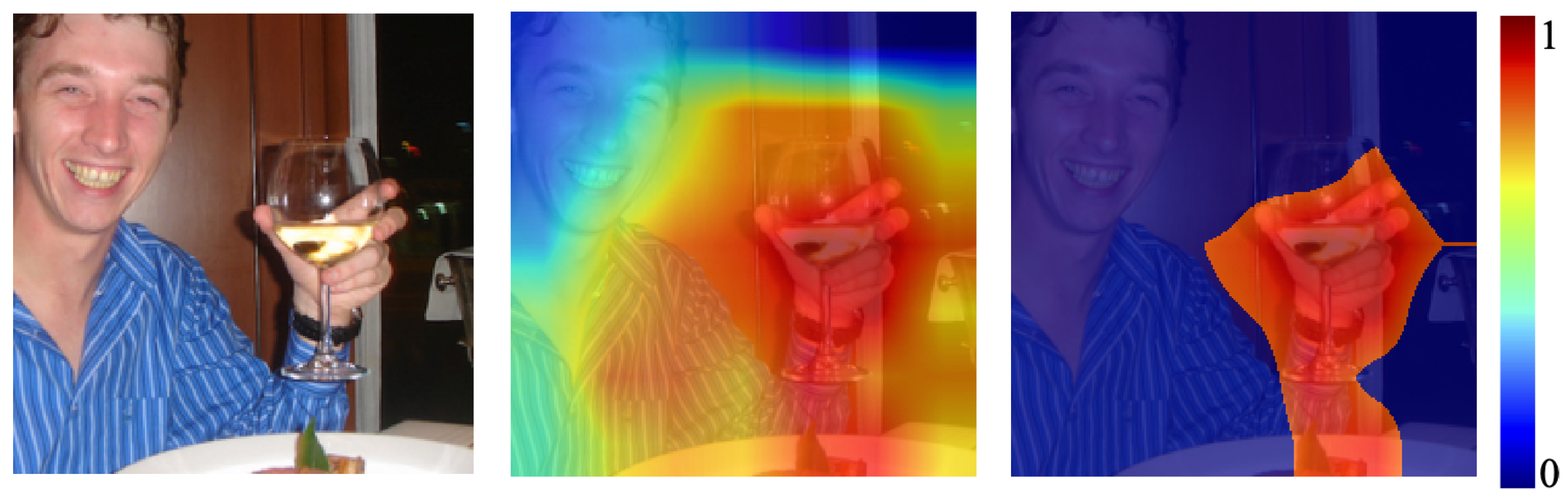
For proper input attribution, we need to deal with two aspects of the problem: detecting important features and assigning appropriate scores representing the relative importance of detected features. Due to the similarity to a detection task of the former aspect, we can conjecture that there can be a false detection of important features by input attribution methods. An example of such false detection is demonstrated in Figure 1 (middle), which shows the attribution map of Grad-CAM [4], one of the most popular input attribution methods, overlaid on an original image from the Pascal VOC dataset [13]. The attribution map is generated for the class “wine glass”. At first glance, one may think that Grad-CAM has well-highlighted regions relevant to the wine glass. However, regions outside of the wine glass have received nonzero relevance scores with respect to the class. As a result, it is unclear where the boundary between relevant and irrelevant regions is.

In fact, many of the current activation-based input attribution methods use naïve forms of relevance thresholding. Table 1 shows the percentage of muted relevance scores in popular activation-based attribution methods, namely Grad-CAM [4], Grad-CAM++ [5], Ablation-CAM [8], and Layer-CAM [9]. However, we found that such thresholding does not always provide good attribution maps that depict relevant regions well—for example, the Grad-CAM attribution map in Figure 1 (middle) shows only the top $15\%$ of the $I_{\mathrm{pre}}$ map of Grad-CAM, but it fails to highlight the specific region corresponding to the wine glass, as we have discussed above. Therefore, we discuss how to perform better thresholding in a structured way to generate attribution maps of higher quality.

4. Methodology

In this section, we first introduce the details of our threshold fine-tuning (TFT) procedure to find an optimal threshold value that maximizes the measure of relative probability increase. Then, we discuss our activation fine-tuning (AFT) strategy to refine the activations of a target CNN with the help of a tuner network and the optimal masks obtained by TFT as auxiliary data.

4.1. Threshold Fine-Tuning Procedure

To find an optimal threshold value that improves the quality of an attribution map, we introduce our threshold fine-tuning procedure.

4.1.1. Thresholding an Attribution Map

Given an attribution map I with respect to an input image x, we define a thresholded attribution map $I_{\tau }$ for a threshold value $\tau \in [0,1]$ as follows:

$${\left[I_{\tau }\right]}_{ij}=\left\{\begin{array}{cc}\hfill I_{ij}\hfill & \hfill \mathrm{if}{I}_{ij}\ge \tau \hfill \\ \hfill 0\hfill & \hfill \mathrm{otherwise}.\hfill \end{array}\right.$$

(4)

Based on $I_{\tau }$, we also define the binary mask $M_{\tau }$:

$${\left[M_{\tau }\right]}_{ij}=\left\{\begin{array}{cc}\hfill 1\hfill & \hfill \mathrm{if}{I}_{ij}\ne 0\hfill \\ \hfill 0\hfill & \hfill \mathrm{otherwise}.\hfill \end{array}\right.$$

(5)

Finally, we define the binary masked version ${\widehat{x}}_{\tau }$ of the input image x, which we use in our algorithm to evaluate the quality of $I_{\tau }$,

$${\widehat{x}}_{\tau }=M_{\tau }\odot x,$$

(6)

where ⊙ is the element-wise multiplication.

4.1.2. Finding an Optimal Threshold

To design an automated procedure for finding an optimal threshold value, we need to check the quality of a thresholded attribution map $I_{\tau }$. This can be done by asking the target classifier we use to generate attribution maps. That is, for a masked input ${\widehat{x}}_{\tau }$ created according to (6), we measure how much the model’s predicted class probability has increased due to masking: our conjecture is that if the masking has been successful, it will remove class-irrelevant features, and therefore the model will output a higher probability for the given class.

To be more specific, we define the relative probability increase (RPI) for the quality measure as follows:

$$\mathrm{RPI}({\widehat{x}}_{\tau },x):=\frac{max\{{\widehat{y}}^c-y^c,0\}}{y^c},$$

(7)

where ${\widehat{y}}^c$ is the prediction probability of a masked input ${\widehat{x}}_{\tau }$ and $y^c$ is the prediction probability of the original image x, with respect to the class c. RPI measures the increase of class probability due to masking, relative to the original probability.

We compute the RPI values for increasing values of $\tau$ so that ${\widehat{x}}_{\tau }$s generated in the process will contain progressively increasing numbers of features. Then, we choose the best $I_{{\tau }^{*}}$ for which we have the largest RPI value. Algorithm 1 shows our procedure, called threshold fine-tuning (TFT), which uses GPU-based batch processing to accelerate the computation of multiple forward passes (the lines 9 to 11 in Algorithm 1).

Algorithm 1: Threshold Fine-Tuning (TFT) Algorithm

Input: an input image x, an attribution map I, and a classifier $f\left(x\right)$ Input: an array T of increasing threshold values in $[0,1]$        1: Initialize RPI as a $\left|T\right|$-dimensional array with the zero values.        2: Initialize $\widehat{X}$ as a $\left|T\right|$-dimensional array with the zero values.        3: for$i=1:\left|T\right|$do        4:     $\tau \leftarrow T\left[i\right]$.        5:     Compute $I_{\tau }$ and ${\widehat{x}}_{\tau }$ according to (4) and (6).        6:     $\widehat{X}\left[i\right]\leftarrow {\widehat{x}}_{\tau }$.        7: end for        8: Transfer $\widehat{X}$ to a GPU.        9: GPUStart                ▹ Batch processing of all masked images at once.        10:     ${\widehat{Y}}^c\leftarrow \mathrm{the}\mathrm{prediction}\mathrm{probability}\mathrm{of}\widehat{X}\mathrm{for}\mathrm{the}\mathrm{class}c$.        11: GPUEnd        12: for$i=1:\left|T\right|$do        13:     $\mathrm{RPI}\left[i\right]\leftarrow$ the quality of ${\widehat{x}}_{\tau }$ according to (7) based on ${\widehat{Y}}^c\left[i\right]$.        14: end for        15: ${\tau }^{*}=T\left[{arg\; max}_{i=1,2,\cdots ,\left|T\right|}\mathrm{RPI}\left[i\right]\right]$.        16: Return $I_{{\tau }^{*}}$.

4.2. Activation Fine-Tuning

In experiments, we show that our threshold fine-tuning (TFT) can produce optimally thresholded attribution maps with significantly higher attribution quality than the original attribution maps. However, one downside is that TFT has to be performed on every input, which can be costly for providing an AI-based inference service with input attribution.

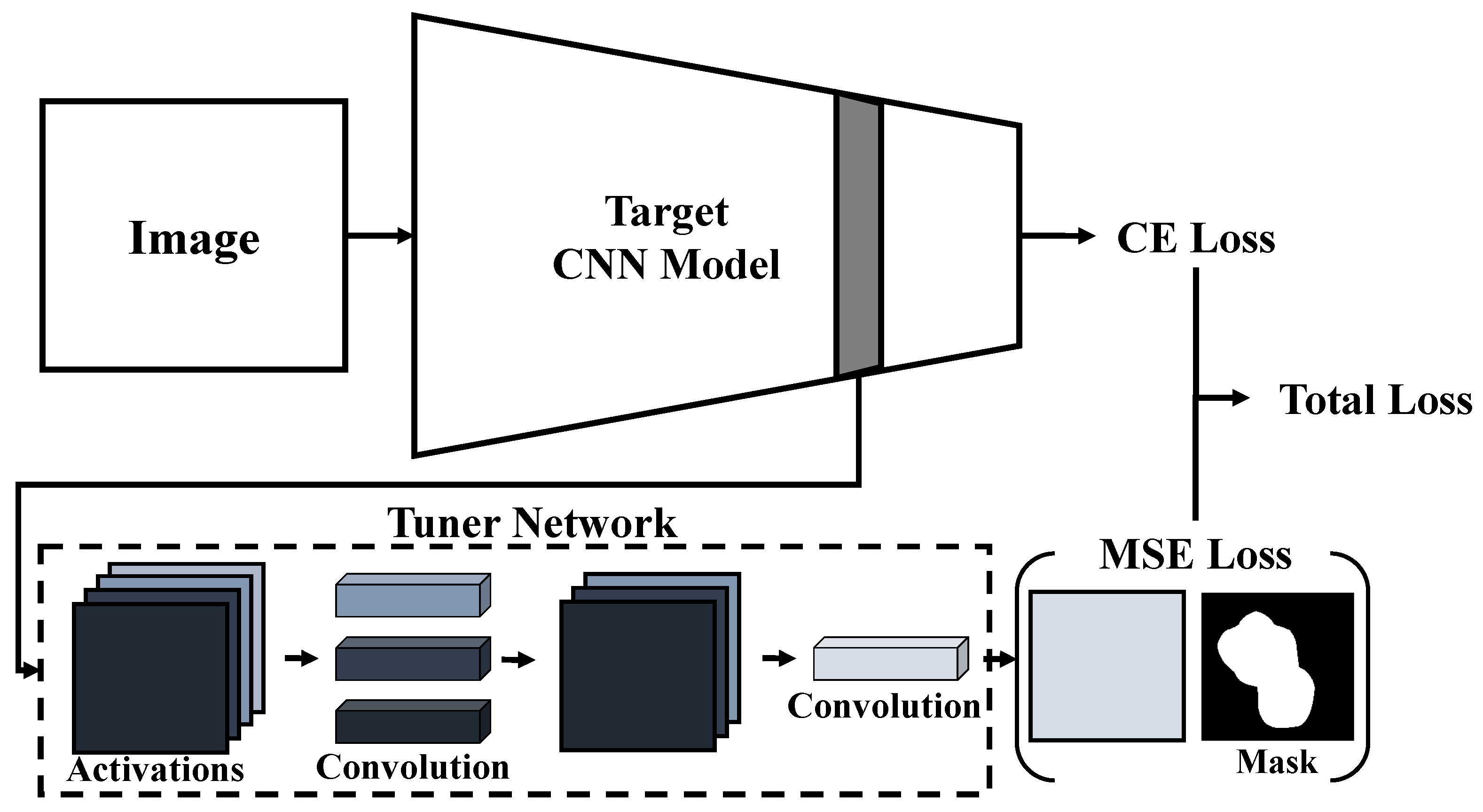
Therefore, we propose an activation fine-tuning (AFT) strategy that uses TFT to generate auxiliary data to adjust the activations of a target CNN so that they will be better suited for creating attribution maps. The idea is that since the optimal masks $M_{{\tau }^{*}}$ contain the information of class-relevant regions in activations, we can use the masks as new data to fine-tune the activations. Figure 2 illustrates our AFT strategy, which takes activations (at a specific layer where we generate input attribution) and uses a tuner network to fit the shape of activations with multiple channels to the masks with no channel information.

4.2.1. Tuner Network

Let us say that the activation A of a target CNN has the shape of $d_h\times d_w\times K$, where $d_h$, $d_w$, and K denotes the height, width, and the number of channels of the activations. To use the optimal mask $M_{{\tau }^{*}}$ of the shape $d_h\times d_w\times 1$ to fine-tune the activation A teaching class-relevant regions, we need to transform the shape of A to that of the optimal mask. In addition, the combination of the K channels will be better to learn since the activation-based attribution methods use the gradient information of the CNN with respect to the activations to construct a weighted combination of A to construct input attribution maps, from which the optimal masks have been computed.

Therefore, we use a tuner network with two layers of $1\times 1$ convolutions, which creates a linear combination of input channels without changing the spatial dimension of input tensors [31]. The network use three $1\times 1$ convolution filters to reduce activations to $H\times W\times 3$ at the first layer (the number of filters has been determined empirically) and then one $1\times 1$ filter to reduce it further to $H\times W\times 1$ as desired.

4.2.2. Optimization Problem for Activation Fine-Tuning

For a training image x, let us denote the target CNN for which we want to create input attribution as $f(x;w)$ and the layer as the ℓ-th layer, where we obtain activations for creating activation-based input attribution and also attach our tuner network. We consider the learning weights w in three parts, namely $w=(w_0,w_1,w_2)$ where $w_0$ corresponds to the first to $(\ell -1)$-th layers, $w_1$ corresponds to the ℓ-th layer, and $w_2$ to the remaining layers. Note that we freeze the weights in $w_0$ to their pre-trained version to prevent the original CNN from fluctuating too much from its optimal weights, losing its best prediction performance. We also denote the activations at the ℓ-th layer as $A(x;w_1)\in {\mathbb{R}}^{d_h\times d_w\times K}$: A depends on both $w_0$ and $w_1$, but only $w_1$ is used for fine-tuning.

For the tuner network $f_{tuner}(A(x;w_1);w^{\prime })$ and the optimal mask $M_{{\tau }^{*}}\left(x\right)$ generated by TFT, we define activation fine-tuning as the following optimization problem:

$$\underset{w_1,w_2,w^{\prime }}{min}\sum _{i=1}^{n_{\mathrm{AFT}}}{\mathcal{L}}_{CE}(f(x_i;w_1,w_2),y_i)+\lambda {\parallel f_{tuner}(A(x_i;w_1);w^{\prime })-M_{{\tau }^{*}}\left(x\right)\parallel }_2^2,$$

(8)

where the input–label pairs $(x_i,y_i)$ are from training data, ${\mathcal{L}}_{CE}$ is the cross-entropy loss, and $\lambda >0$ is a hyper-parameter balancing the strength of the tuner network.

5. Experiments

In our experiments, we applied our method on two large-scale CNNs: ResNet-50 [32] and VGG-16 [33]. We used ImageNet [12], and Pascal VOC 2012 [13] datasets, two popular datasets for object classification. For TFT experiments, we used pre-trained models of ResNet-50 and VGG-16. For AFT experiments, we retrained the pre-trained models using the original training sets of the two datasets and additional data created by applying TFT on the training data. All performance numbers have been measured on the test sets of the two datasets, summarized in

Table 2. The summary of datasets used in the experiments.

Dataset	# Train	# Test	# Classes
ImageNet [12]	1,281,167	10,000	1000
Pascal VOC 2012 [13]	1464	1449	20

.

We implemented our method with PyTorch and tested against the four activation-based input attribution methods, namely Grad-CAM [4], Grad-CAM++ [5], Ablation-CAM [8], and Layer-CAM [9]. Our implementation is available in an open-source format at https://github.com/sanglee/AFT (accessed on 14 September 2022).

5.1. Qualitative Comparison of Original and Optimally Thresholded Attribution Maps

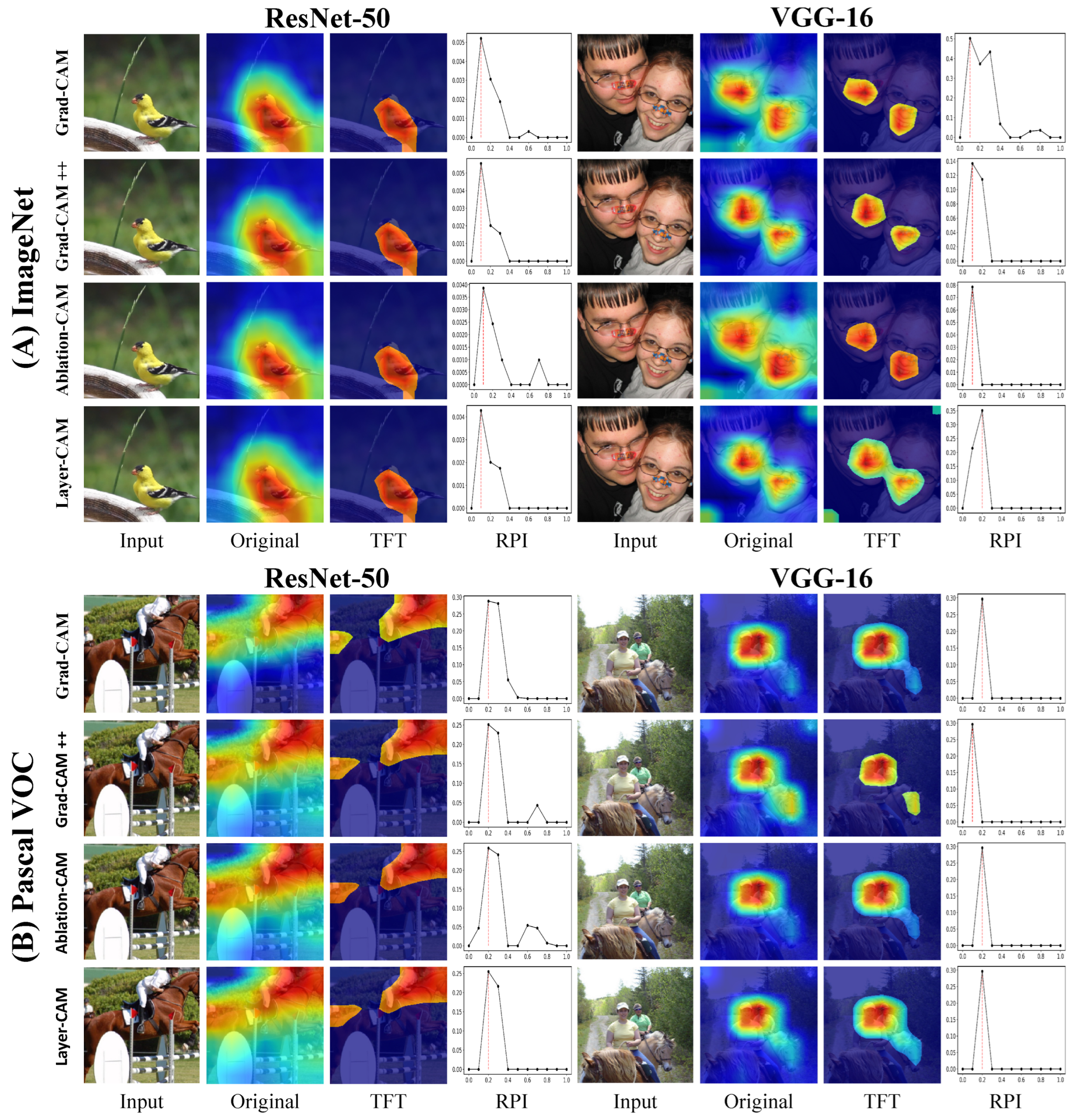
To show the effectiveness of our threshold fine-tuning (TFT) algorithm, we compared the original attribution maps with optimally thresholded attribution maps generated by TFT. For the comparison, we have chosen several images from each dataset and generated attribution maps. We have applied our TFT algorithm to the attribution maps, computing the RPI values over increasing threshold values in $[0,1]$ with an increment of $0.1$. The attribution maps were thresholded to maximize the RPI measure. Figure 3 shows the results in the order of the input image, the original attribution map I without thresholding, the thresholded attribution map $I_{{\tau }^{*}}$, and a curve of RPI values (y-axis) over increasing threshold values (x-axis) indicating the best threshold ${\tau }^{*}$ with vertical dotted lines.

In Figure 3, we can observe that (i) the best threshold values are different depending on the datasets, networks, and images, although the best threshold values were similar across different attribution methods for a specific network and image combination; (ii) most of the RPI curves have prominent peaks so that we can find the maximum point; and (iii) our thresholding does make the boundary of highlighted regions more apparent, which will be beneficial for finding important regions, parts, or objects.

5.2. Quantitative Improvements of Attribution Maps

To show that our TFT and AFT can improve the quality of input attribution, we compared the quality of attribution maps generated by the original model, TFT and AFT. For the comparison, we computed attribution quality measures widely used in model induction-based XAI research in image domains: average increase and average drop. Denoting by $y_i^c$ the predicted probability of the original input $x_i$ for the class c, by ${\widehat{y}}_i^c$ the predicted probability for the class c of the binary-masked image ${\left({\widehat{x}}_{\tau }\right)}_i$ based on a thresholded attribution map ${\left(I_{\tau }\right)}_i$, and by $y_i$ the true label, we define the attribution quality measures as follows [5]:

$$\begin{array}{cc}\hfill \mathrm{Average}\mathrm{Increase}=& \frac{1}{n}\sum _{i=1}^n\mathbf{1}[{\widehat{y}}_i^c>y_i^c]\hfill \\ \hfill \mathrm{Average}\mathrm{Drop}=& \hfill \frac{1}{n}\sum _{i=1}^{n}max\{y_i^c-{\widehat{y}}_i^c,0\}/y_i^c,\hfill \end{array}$$

where $\mathbf{1}\left[z\right]$ has the value 1 if z is true and 0 otherwise.

Table 3. Comparison of the quality of attribution maps: the original attribution maps (Original), the original attribution maps optimized by the threshold fine-tuning (TFT), and the attribution maps generated with the CNN optimized by the activation fine-tuning (AFT) without any threshold fine-tuning. The numbers in boldfaces indicate performance improvements over the original cases.

Dataset	Attribution Method	Measure	ResNet-50			VGG-16
			Original	TFT	AFT	Original	TFT	AFT
ImageNet	Grad-CAM	Avg Increase	0.334	0.439 (×1.32)	0.449 (×1.35)	0.294	0.385 (×1.31)	0.561 (×1.91)
		Avg Drop	0.130	0.117 (×1.11)	0.116 (×1.11)	0.159	0.144 (×1.10)	0.124 (×1.28)
	Grad-CAM++	Avg Increase	0.342	0.454 (×1.33)	0.507 (×1.48)	0.228	0.322 (×1.42)	0.505 (×2.22)
		Avg Drop	0.136	0.123 (×1.11)	0.105 (×1.29)	0.188	0.174 (×1.08)	0.153 (×1.23)
	Ablation-CAM	Avg Increase	0.342	0.456 (×1.33)	0.514 (×1.50)	0.261	0.352 (×1.35)	0.496 (×1.90)
		Avg Drop	0.137	0.123 (×1.12)	0.109 (×1.25)	0.173	0.159 (×1.09)	0.136 (×1.27)
	Layer-CAM	Avg Increase	0.340	0.452 (×1.33)	0.512 (×1.50)	0.230	0.325 (×1.42)	0.492 (×2.14)
		Avg Drop	0.128	0.124 (×1.11)	0.104 (×1.33)	0.187	0.172 (×1.09)	0.150 (×1.25)
Pascal VOC	Grad-CAM	Avg Increase	0.546	0.679 (×1.24)	0.659 (×1.21)	0.569	0.670 (×1.17)	0.698 (×1.23)
		Avg Drop	0.055	0.045 (×1.20)	0.037 (×1.46)	0.054	0.045 (×1.20)	0.053 (×1.02)
	Grad-CAM++	Avg Increase	0.522	0.674 (×1.29)	0.618 (×1.18)	0.445	0.583 (×1.31)	0.618 (×1.39)
		Avg Drop	0.059	0.046 (×1.28)	0.041 (×1.43)	0.067	0.056 (×1.20)	0.062 (×1.08)
	Ablation-CAM	Avg Increase	0.523	0.682 (×1.31)	0.666 (×1.27)	0.519	0.638 (×1.23)	0.674 (×1.30)
		Avg Drop	0.049	0.036 (×1.34)	0.033 (×1.48)	0.052	0.044 (×1.18)	0.050 (×1.03)
	Layer-CAM	Avg Increase	0.486	0.645 (×1.33)	0.620 (×1.28)	0.420	0.538 (×1.28)	0.562 (×1.34)
		Avg Drop	0.063	0.051 (×1.23)	0.042 (×1.52)	0.069	0.058 (×1.19)	0.059 (×1.16)

shows the comparison results for attribution quality. Higher values are better for the average increase, while lower values are better for the average drop. We can see that TFT improves the quality of attribution maps in all quality measures. Compared to the original cases, the attribution maps optimized by TFT have improved the average increase and average drop by $\times 1.31$ and $\times 1.16$ on average, respectively. Interestingly, the attribution maps generated with AFT-tuned CNN show similar improvements in the two quality measures by $\times 1.51$ and $\times 1.26$ on average, respectively, compared to the original attribution maps. In the case of AFT, activation tuning has been done with the optimal masks generated with the same attribution method to be used for the attribution quality assessment, and no threshold fine-tuning has been applied. Still, using AFT, we achieved an attribution quality similar to (sometimes better than) TFT, except for a few cases in the Pascal VOC dataset.

5.3. Impact of AFT on Prediction Performance

Since our AFT can modify the optimal learning parameters of the original CNN, one concern will be that the prediction accuracy of the CNN may drop due to the application of AFT. Therefore, to check the impact of AFT on the classification accuracy of the AFT-tuned CNN, we compared the accuracy rate of the original and the AFT-tuned models in

Table 4. Comparison of test set prediction accuracy rates of the original and the AFT-tuned CNNs.

Dataset	Attribution Method	ResNet-50		VGG-16
		Original	AFT-Tuned	Original	AFT-Tuned
ImageNet	Grad-CAM	0.737	0.736	0.720	0.720
	Grad-CAM++		0.737		0.718
	Ablation-CAM		0.737		0.720
	Layer-CAM		0.736		0.719
Pascal VOC	Grad-CAM	0.922	0.922	0.905	0.904
	Grad-CAM++		0.923		0.903
	Ablation-CAM		0.922		0.903
	Layer-CAM		0.922		0.904

, for all combinations of the datasets, CNNs, and attribution methods we have tried.

The results show that AFT consistently preserves the original model’s prediction performance, keeping the accuracy rates within $0.002$ percentage points of the original accuracy rates in all cases. Therefore, we expect that AFT can be applied to CNNs without significantly sacrificing the original prediction accuracy.

5.4. Computational Cost of TFT

In Algorithm 1, the bottleneck is computing the RPI scores for masked images at different threshold values, where each of them requires a forward pass of the target CNN to produce prediction probability for the class c for each masked image. We have tried 10 different threshold values in our experiments, and therefore a serial evaluation of the prediction probabilities requires an equal number of forward passes. To curtail runtime, we have adopted GPU-based batch processing to calculate the prediction probabilities for all masked images at once (lines 9–11 of Algorithm 1).

In

Table 5. Average runtime (in seconds) of generating an attribution map with and without our uncovering procedure using VGG-16. The Δ indicates the difference between the two cases.

	Grad-CAM	Grad-CAM++	Ablation-CAM	Layer-CAM
Without	$0.017$	$0.017$	$1.691$	$0.018$
With	$0.045$	$0.046$	$1.719$	$0.047$
Δ	$0.028$	$0.029$	$0.028$	$0.029$

, we show the runtime to create an input attribution map with and without our TFT. The measurements are conducted on a load-free Linux machine with an Intel CPU Xeon Silver 4214 CPU, an NVIDIA RTX 2080 Ti GPU, and 128 GB of RAM. The results show that our method takes less than $0.03$ seconds across all cases in our experimental environment, which we believe allowable considering the runtime of attribution map creation themselves and the expected quality improvement due to TFT.

6. Conclusions

In this paper, we proposed novel ways to replace the ad-hoc thresholding of attribution scores in activation-based input attribution approaches, which can cause the quality degradation of input attribution maps. First, we proposed the threshold fine-tuning (TFT) procedure to optimize the cut-off thresholds of attribution scores, showing that applying fine-tuned thresholds can significantly improve the quality of attribution. Secondly, we provided the activation fine-tuning (AFT) strategy using a tuner network trained by the output of TFT as auxiliary training data to regulate the activations of a CNN. As a result, AFT-tuned CNN produces activations that do not require further per-input attribution thresholding to generate activation-based input attribution. Furthermore, we have shown that AFT does not sacrifice the prediction accuracy of the target CNN. Therefore, AFT can make activation-based input attribution methods more plausible whenever providing input attribution is necessary to get more information about decision-making by CNN models.

The effectiveness of our method indicates that the activation-based attribution methods may assign nonzero relevance scores to some class-irrelevant features. We think that several factors could be involved and deserve further investigation. First, gradient computation can be noisy. The non-differentiability of activation functions such as ReLU may have introduced noise in gradient computation. Second, the inaccuracy of the underlying CNN classifier may have resulted in an incorrect evaluation of activation values. Since the effect of these factors can be combined, further research will be needed to determine the exact causes and find proper remedies to improve attribution methods.

Several aspects of this study can be improved in future works. First, our TFT and AFT methods consider only a single activation layer of a CNN—the last convolutional layer in particular. The reason is that most activation-based input attribution methods use the output of the last convolutional layer to generate input attribution maps. However, a few recent techniques, such as Layer-CAM [9], suggest that information from multiple convolutional layers helps improve input attribution. Therefore, extending our AFT approach to tune multiple convolutional layers together will be a worthwhile research direction. Second, there are a few hyperparameters in our approach, such as the number of threshold values T in Algorithm 1, the number of training examples to be used for activation fine-tuning $n_{\mathrm{AFT}}$, and the balancing parameter $\lambda$ in (8). Although these hyperparameters have not been very sensitive in our experiment, it would require further investigation into other datasets and neural networks than those we have tried in this study.

References

- DARPA-XAI. Explainable Artificial Intelligence (XAI), DARPA-BAA-16-53; Defense Advanced Research Projects Agency: Arlington County, VA, USA, 2016.
- EU-GDPR. EU General Data Protection Regulation: Regulation (EU) 2016/679 of the European Parliament and of the Council of 27 April 2016 on the Protection of Natural Persons with Regard to the Processing of Personal Data and on the Free Movement of Such Data, and Repealing Directive 95/46/EC (General Data Protection Regulation), OJ 2016 L 119/1; European Commission: Brussels, Belgium, 2016. [Google Scholar]
- Zhou, B.; Khosla, A.; Lapedriza, A.; Oliva, A.; Torralba, A. Learning Deep Features for Discriminative Localization. In Proceedings of the IEEE Conference on Computer Vision and Pattern Recognition (CVPR), Las Vegas, NV, USA, 27–30 June 2016; pp. 2921–2929. [Google Scholar]
- Selvaraju, R.R.; Cogswell, M.; Das, A.; Vedantam, R.; Parikh, D.; Batra, D. Grad-CAM: Visual Explanations From Deep Networks via Gradient-Based Localization. In Proceedings of the IEEE International Conference on Computer Vision (ICCV), Venice, Italy, 22–29 October 2017; pp. 618–626. [Google Scholar]
- Chattopadhay, A.; Sarkar, A.; Howlader, P.; Balasubramanian, V.N. Grad-CAM++: Generalized Gradient-Based Visual Explanations for Deep Convolutional Networks. In Proceedings of the 2018 IEEE Winter Conference on Applications of Computer Vision (WACV), Lake Tahoe, NV, USA, 12–15 March 2018; pp. 839–847. [Google Scholar]
- Wang, H.; Wang, Z.; Du, M.; Yang, F.; Zhang, Z.; Ding, S.; Mardziel, P.; Hu, X. Score-cam: Score-weighted visual explanations for convolutional neural networks. In Proceedings of the IEEE/CVF Conference on Computer Vision and Pattern Recognition Workshops, Seattle, WA, USA, 14–19 June 2020; pp. 24–25. [Google Scholar]
- Lee, J.R.; Kim, S.; Park, I.; Eo, T.; Hwang, D. Relevance-CAM: Your Model Already Knows Where To Look. In Proceedings of the IEEE/CVF Conference on Computer Vision and Pattern Recognition (CVPR), Nashville, TN, USA, 20–25 June 2021; pp. 14944–14953. [Google Scholar]
- Desai, S.; Ramaswamy, H.G. Ablation-CAM: Visual Explanations for Deep Convolutional Network via Gradient-free Localization. In Proceedings of the IEEE/CVF Winter Conference on Applications of Computer Vision (WACV), Snowmass Village, CO, USA, 1–5 March 2020; pp. 983–991. [Google Scholar]
- Jiang, P.T.; Zhang, C.B.; Hou, Q.; Cheng, M.M.; Wei, Y. Layercam: Exploring hierarchical class activation maps for localization. IEEE Trans. Image Process. 2021, 30, 5875–5888. [Google Scholar] [CrossRef]
- Zhang, Q.; Rao, L.; Yang, Y. A Novel Visual Interpretability for Deep Neural Networks by Optimizing Activation Maps with Perturbation. In Proceedings of the AAAI Conference on Artificial Intelligence, Vancouver, BC, Canada, 2–9 February 2021; Volume 35, pp. 3377–3384. [Google Scholar]
- Adebayo, J.; Gilmer, J.; Muelly, M.; Goodfellow, I.; Hardt, M.; Kim, B. Sanity Checks for Saliency Maps. In Proceedings of the Advances in Neural Information Processing Systems, Montréal, QC, Canada, 3–8 December 2018; Bengio, S., Wallach, H., Larochelle, H., Grauman, K., Cesa-Bianchi, N., Garnett, R., Eds.; Curran Associates, Inc.: Red Hook, NY, USA, 2018; Volume 31. [Google Scholar]
- Russakovsky, O.; Deng, J.; Su, H.; Krause, J.; Satheesh, S.; Ma, S.; Huang, Z.; Karpathy, A.; Khosla, A.; Bernstein, M.; et al. ImageNet Large Scale Visual Recognition Challenge. Int. J. Comput. Vis. (IJCV) 2015, 115, 211–252. [Google Scholar] [CrossRef] [Green Version]
- Everingham, M.; Van Gool, L.; Williams, C.K.I.; Winn, J.; Zisserman, A. The Pascal Visual Object Classes (VOC) Challenge. Int. J. Comput. Vis. 2010, 88, 303–338. [Google Scholar] [CrossRef] [Green Version]
- Erhan, D.; Bengio, Y.; Courville, A.; Vincent, P. Visualizing Higher-Layer Features of a Deep Network; University of Montreal: Montreal, QC, Canada, 2009; Volume 1341, p. 1. [Google Scholar]
- Baehrens, D.; Schroeter, T.; Harmeling, S.; Kawanabe, M.; Hansen, K.; Müller, K.R. How to Explain Individual Classification Decisions. J. Mach. Learn. Res. 2010, 11, 1803–1831. [Google Scholar]
- Oquab, M.; Bottou, L.; Laptev, I.; Sivic, J. Learning and transferring mid-level image representations using convolutional neural networks. In Proceedings of the IEEE Conference on Computer Vision and Pattern Recognition, Columbus, OH, USA, 23–28 June 2014; pp. 1717–1724. [Google Scholar]
- Zeiler, M.D.; Fergus, R. Visualizing and Understanding Convolutional Networks. In Proceedings of the European Conference on Computer Vision, Zurich, Switzerland, 6–12 September 2014; pp. 818–833. [Google Scholar]
- Ribeiro, M.T.; Singh, S.; Guestrin, C. “Why Should I Trust You?”: Explaining the Predictions of Any Classifier. In Proceedings of the 22nd ACM SIGKDD International Conference on Knowledge Discovery and Data Mining, San Francisco, CA, USA, 13–17 August 2016; pp. 1135–1144. [Google Scholar]
- Lundberg, S.M.; Lee, S.I. A Unified Approach to Interpreting Model Predictions. In Proceedings of the Advances in Neural Information Processing Systems, Long Beach, CA, USA, 4–9 December 2017; Guyon, I., Luxburg, U.V., Bengio, S., Wallach, H., Fergus, R., Vishwanathan, S., Garnett, R., Eds.; Curran Associates, Inc.: Red Hook, NY, USA, 2017; Volume 30. [Google Scholar]
- Sundararajan, M.; Dhamdhere, K.; Agarwal, A. The Shapley Taylor Interaction Index. In Proceedings of the 37th International Conference on Machine Learning, Virtual, 13–18 July 2020; PMLR: Vienna, Austria, 2020; Voume 119, pp. 9259–9268. [Google Scholar]
- Petsiuk, V.; Das, A.; Saenko, K. RISE: Randomized Input Sampling for Explanation of Black-box Models. In Proceedings of the British Machine Vision Conference (BMVC), Newcastle, UK, 3–6 September 2018. [Google Scholar]
- Kapishnikov, A.; Bolukbasi, T.; Viegas, F.; Terry, M. XRAI: Better Attributions Through Regions. In Proceedings of the 2019 IEEE/CVF International Conference on Computer Vision (ICCV), Seoul, Republic of Korea, 27 October–2 November 2019; pp. 4947–4956. [Google Scholar]
- Springenberg, J.T.; Dosovitskiy, A.; Brox, T.; Riedmiller, M. Striving for Simplicity: The All Convolutional Net. In Proceedings of the ICLR (Workshop Track), San Diego, CA, USA, 7–9 May 2015. [Google Scholar]
- Sundararajan, M.; Taly, A.; Yan, Q. Axiomatic Attribution for Deep Networks. In Proceedings of the 34th International Conference on Machine Learning, Sydney, Australia, 6–11 August 2017; PMLR: Sydney, Australia, 2017; Volume 70, pp. 3319–3328. [Google Scholar]
- Shrikumar, A.; Greenside, P.; Kundaje, A. Learning Important Features Through Propagating Activation Differences. In Proceedings of the 34th International Conference on Machine Learning, Sydney, Australia, 6–11 August 2017; Precup, D., Teh, Y.W., Eds.; PMLR: Sydney, Australia, 2017; Volume 70, pp. 3145–3153. [Google Scholar]
- Balduzzi, D.; Frean, M.; Leary, L.; Lewis, J.P.; Ma, K.W.D.; McWilliams, B. The Shattered Gradients Problem: If resnets are the answer, then what is the question? In Proceedings of the 34th International Conference on Machine Learning, Sydney, Australia, 6–11 August 2017; PMLR: Sydney, Australia, 2017; Volume 70, pp. 342–350. [Google Scholar]
- Bach, S.; Binder, A.; Montavon, G.; Klauschen, F.; Müller, K.R.; Samek, W. On Pixel-Wise Explanations for Non-Linear Classifier Decisions by Layer-Wise Relevance Propagation. PLoS ONE 2015, 10, e0130140. [Google Scholar] [CrossRef] [Green Version]
- Montavon, G.; Samek, W.; Müller, K.R. Methods for interpreting and understanding deep neural networks. Digit. Signal Process. 2018, 73, 1–15. [Google Scholar] [CrossRef]
- Gu, J.; Yang, Y.; Tresp, V. Understanding individual decisions of CNNs via contrastive backpropagation. In Proceedings of the Asian Conference on Computer Vision; Springer: Berlin/Heidelberg, Germany, 2018; pp. 119–134. [Google Scholar]
- Nam, W.; Choi, J.; Lee, S. Relative Attributing Propagation: Interpreting the Comparative Contributions of Individual Units in Deep Neural Networks. In Proceedings of the Association for the Advancement of Artificial Intelligence, AAAI’20, New York, NY, USA, 7–12 February 2020. [Google Scholar]
- Lin, M.; Chen, Q.; Yan, S. Network In Network. In Proceedings of the International Conference on Learning Representations, Banff, AB, Canada, 14–16 April 2014. [Google Scholar]
- He, K.; Zhang, X.; Ren, S.; Sun, J. Deep Residual Learning for Image Recognition. In Proceedings of the IEEE Conference on Computer Vision and Pattern Recognition, Las Vegas, NV, USA, 27–30 June 2016; pp. 770–778. [Google Scholar]
- Simonyan, K.; Zisserman, A. Very Deep Convolutional Networks for Large-Scale Image Recognition. In Proceedings of the 3rd International Conference on Learning Representations, ICLR 2015, San Diego, CA, USA, 7–9 May 2015. [Google Scholar]