Analysis of Edge Method Accuracy and Practical Multidirectional Modulation Transfer Function Measurement

Abstract

The modulation transfer function (MTF) is commonly used as an imaging quality criterion reflecting the spatial resolution capability of imaging systems. The modified edge methods based on ISO Standard 12233 are widely used in MTF measurement for various imaging fields with high confidence. However, there are two problems in the existing edge methods which limit the application in remote sensing (RS) field with complicated image quality and usually uncontrollable edge angle: a near-horizontal or near-vertical “small tilt angle straight (STAS)” edge is required, and the MTF measurement results show low robustness and non-uniqueness. In this study, the influence of edge angle, oversampling rate (OSR), region of interest (ROI), edge contrast, and random noise on the edge method accuracy is quantitatively analyzed, and a practical multidirectional MTF measurement edge method is proposed based on the above analysis results. The modified edge method adaptively determines the optimal OSR according to edge angle and combines multiple measurement states, such as multi-ROI extraction and multi-phase binning, to improve the robustness, accuracy, and practicality of the edge method.

1. Introduction

In order to ensure the effective working state of an optical RS imaging system, it is necessary to monitor its on-orbit imaging performance in real-time. Spatial resolution represents the ability to capture or distinguish fine spatial details, and it is closely related to the Ground Sampling Distance (GSD) and the Instantaneous Field of View (IFOV) [1]. However, the spatial resolution is more complicated than the concept of GSD or IFOV. Most agree that the effective spatial resolution is due to three features of the sensor: the instantaneous field of view (IFOV), the MTF, and the signal-to-noise ratio (SNR) [1]. Moreover, MTF is the most commonly used imaging quality assessment indicator for various imaging fields.

MTF is used to characterize the ability to faithfully reproduce the scene spatial frequency content of an imaging system or its components [2]. The imaging system for MTF analysis must be approximately linear and shift invariant. Furthermore, to preserve the convenience of the transfer function approach for a sampled imaging system, it is assumed that the target being imaged has spatial frequency components with random phases that are uniformly distributed with respect to the sampling sites [2]. For a sampled imaging system, it is convenient to express the unit of spatial frequency as line pair/pixel (lp/pix) with the Nyquist and sampling cutoff frequencies corresponding to 0.5 lp/pix and 1 lp/pix, respectively. According to the different structural characteristics of the target, MTF measurement methods mainly include the point source method, pulse method, edge method, and contrast method, which involve the analysis of the responses of points, lines, edges, and periodic bar patterns in the target image. Point source and pulse methods are closest to the MTF definition in principle, but the used target size of the point and line affects the accuracy of MTF measurement, which limits the application in orbit. The contrast method is mostly used for laboratory measurements due to the demand for periodic stripe targets, which is usually easy to realize in the laboratory. Among them, the edge method has high practicability and the widest application, which is not only widely used for laboratory measurements under various implementation manners but also has been used for numerous space sensors in orbit [1,3]. The existing modified edge methods are mainly based on ISO 12233: 2017 e-SFR algorithm [4]. The ISO 12233 standard, which is also known as the edge method, slanted-edge method, or knife-edge method, is intended to characterize the spatial resolution of digital still cameras with two-dimensional photo element arrays that respond to light in proportion to the intensity of the light. The spatial frequency response is measured to approximate the MTF as a function of the horizontal or vertical spatial frequency by analyzing a near-vertical or near-horizontal bi-tonal edge image, respectively. However, it cannot be directly used for multidirectional MTF estimation.

Recently, research into the edge method has mainly focused on improving the accuracy and practicability of MTF measurement. Relevant scholars pay more attention to the following five topics: the accurate and stable detection of edge angle, the accurate and effective construction of Edge Spread Function (ESF), the accuracy and error analysis of edge method, the practical research of MTF measurement method, and the transformation and acquisition of MTF [5,6]. Edge detection mainly adopts the row difference method [4] or the parameter fitting method [2]. ESF construction mainly adopts discrete oversampled binning method [4,7] or appropriate model fitting method [3,8,9]. The application of the model fitting method is an effective and excellent means for accurate edge detection and ESF construction, which is more suitable for the field of ground image processing than aerospace on-orbit processing. The research on the accuracy and error analysis of the edge method is comprehensive and in-depth [10,11,12,13]. It is basically determined that the factors affecting the accuracy of the edge method include edge angle, OSR, binning phase shift (PS), random noise, edge contrast, spatial resolution, etc. The practical research on the MTF measurement algorithm has great application significance. Dr. Masaoka has made continuous and in-depth research on the edge method and its practical improvement [2,7,11,14,15,16] and has made some progress in multidirectional MTF measurement, coupling relationship between edge angle, OSR and binning PS, variable OSR model, etc. Moreover, the Infrared and Visible Optical Sensors (IVOS) team from various countries and professional entities has conducted comparative research on MTF measurement and provided open edge reference data sets to construct an exchange platform for effectively improving edge methods [1]. Zengilowski et al. studied the adaptive improved edge method for the MTF measurement of an infrared imaging system [17]. Wang et al. used MTF measured by the edge method as a prior term for remote sensing image restoration [18]. MTF measurement technology using the edge method is also widely used to analyze the spatial resolution characteristics of optical systems in different fields such as medicine, aerospace, and so on [19,20].

However, the edge method is still restricted by the STAS edge requirement, the low robustness, and the non-uniqueness of the measurement results. When RS satellites image natural objects or targets, it is difficult to obtain images containing STAS edges. Fang et al. made use of multi-angle edges to carry out MTF measurement research and pointed out in the prospect that it is necessary to deepen it [21]. The imaging capability of the RS imaging system in the whole field of view is anisotropic, so its MTF(f) is also multidirectional. In fact, the STAS condition in ISO 12233 is proposed for measuring MTF in two specific directions, horizontal or vertical. It should be noted that the projection of ROI to the horizontal direction or the direction perpendicular to the edge does not affect the binning process of oversampled ESF construction, nor the MTF result obtained by the Fast Fourier Transform (FFT), but the different projection directions will affect the actual sampling interval, thus affecting the accurate calculation of spatial frequencies (SF), and finally affecting the accurate matching of MTF measured values with SF. There are still some problems to be explored: Does the STAS edge suggested in ISO 12233 refer to a certain angle or a certain angle range? How do the size and location of ROI affect the accuracy of the edge method? Can the influence of low edge contrast and SNR on edge method accuracy be quantified? How to improve the robustness of the edge method and make it suitable for MTF measurement in various imaging fields?

To overcome the aforementioned issues, in this paper, the influence of edge angle, OSR, ROI, edge contrast, and random noise on the edge method accuracy is quantitatively analyzed, and a practical multidirectional MTF measurement edge method is proposed based on the above analysis results. The main contribution of this work is summarized below.

(1)

The main factors that affect the accuracy of the edge method, such as edge angle, OSR, ROI, edge contrast, and random noise, are quantitatively simulated and analyzed so as to provide a universal parameter determination reference for edge method application in RS imaging fields.

(2)

To further solve the problem of stability, accuracy, and practicability of multidirectional MTF measurement by edge method, according to the quantitative analysis results of influencing factors, an adaptive determination model of optimal OSR and binning PS based on edge angle is proposed. An automatic ROI extraction model of multi-position & multi-size based on edge angle & image size is proposed. By coupling the measurement states of multi-ROI extraction and multi-PS binning, the robustness, accuracy, and practicability of the edge method are comprehensively improved.

The rest of the paper is organized as follows. Section 2 introduces the conventional edge-based MTF measurement methods. Section 3 conducts the analysis of edge method accuracy. Section 4 describes the proposed practical multidirectional MTF measurement method. Section 5 presents the experimental results and analyses. Section 6 presents the discussions and concludes the paper.

2. Conventional Edge-Based MTF Measurement Methods

2.1. Imaging Degradation Process of Edge Target

The optical RS imaging system can be considered a linear system with spatial shift invariant versus radiance. According to the theory of imaging, the image obtained by a linear spatial shift-invariant imaging system can be represented by the convolution of the imaging system’s response and object target. Considering the noise, the imaging process in the spatial domain and spatial frequency domain can be expressed as the following equations according to the convolution theorem:

$$i(x,y)=l(x,y)\otimes h(x,y)+n(x,y)$$

(1)

$$I(f_x,f_y)=L(f_x,f_y)\cdot OTF(f_x,f_y)+N(f_x,f_y)$$

(2)

where $i(x,y)$ represents the image target, $l(x,y)$ represents the object target, $h(x,y)$ is the Point Spread Function (PSF) of the imaging system, $n(x,y)$ represents the additive noise, $\otimes$ is the convolution operator, $I(f_x,f_y)$, $L(f_x,f_y)$, $OTF(f_x,f_y)$, $N(f_x,f_y)$ stands for the Fourier Transform of $i(x,y)$, $l(x,y)$, $h(x,y)$, $n(x,y)$, respectively. $OTF(f_x,f_y)$ is called the Optical Transfer Function (OTF, complex function), and its modulus is MTF.

The object target in the edge method can be approximated as the Heaviside step function, which is expressed by $hea(x)$ or $hea(y)$ [1]:

$$l(x,y)=a\cdot hea(x)\cdot unit(y)+b\cdot unit(x)\cdot unit(y)$$

(3)

where $hea(x)$ is the Heaviside step function centered on, $x=0, unit(x)=1$ for all values of x, b, and a + b represents the pixel values on both sides of the edge.

Moreover, for sensors using a CCD in the image plane, the system is no longer strictly shift-invariant; it is necessary to take sampling into account. Generally, the Dirac comb sampling function $comb(x/p_x,y/p_y)$ is used to represent the discrete sampling effect of CCD, where $p_x$ is the size of IFOV and $p_y$ is the GSD of the push broom imaging system.

To sum up, after blurring, noise, and sampling degradation, the model of the edge target imaging process in the x-direction spatial domain and spatial frequency domain is as follows:

$$i(x)=ESF(x)=\left\{[a\cdot hea(x)+b\cdot unit(x)]\otimes LSF(x)+n(x)\right\}\cdot comb(x/p_x)$$

(4)

$$I(f_x)=\left\{[a\cdot Hea(f_x)+b\cdot \delta (f_x)]\cdot OTF(f_x)+N(f_x)\right\}\otimes Comb(f_x/f_{sx})$$

(5)

where $LSF(x)$ is the cross-sectional curve of $PSF(x,y)$ in the x direction, and $f_{sx}=1/p_x$ is the sampling frequency for the $f_x$ axis.

2.2. MTF Measurement Process of Edge Method

Over-sparse ESF obtained from absolute vertical edge images will cause MTF spectrum aliasing. The problem can be solved by rotating the vertical edge target by θ angle relative to the pixel column of the imaging device. It is assumed that the sampling interval of the detector in both horizontal and vertical directions is p. If all the sampling points are projected on the coordinate axis perpendicular to the edge, the sampling interval in the horizontal and vertical directions become p·cos θ and p·sin θ, respectively. For the slanted edge method, the ESF sampling interval is ε as follows (The schematic diagram of ε is given in document [5]):

$$\epsilon =\left\{\begin{array}{c}p\sin \theta \\ p\cos \theta \end{array}\right.\begin{array}{c}\\ \end{array}\begin{array}{c}(0<\theta <\pi /4)\\ (\pi /4<\theta <\pi /2)\end{array}$$

(6)

Theoretically, by adjusting the edge angle θ, an oversampled ESF(x) with an arbitrarily small sampling interval can be obtained. After one-dimensional comb function sampling, the expression of ESF can be obtained as follows: (The following equation is simplified on the basis of Equation (4), in which the heaviside step function is briefly referred to as step(x), the noise term n(x) is omitted in order to ease the reading of equation, and the comb sampling interval p_x in the horizontal direction is replaced by ε in Equation (6).)

$$\begin{array}{ll}ESF(x)& =\left[step(x)\otimes h(x)\right]\cdot comb(x/\epsilon )\\ & {{}_{}}_{}{{}_{}}_{}{{}_{}}_{}{{}_{}}_{}{{}_{}}_{}{}_{}=\left[step(x)\otimes h(x)\right]\cdot \left[\epsilon {\displaystyle \sum _{n=-\infty }^{\infty }\delta (x-n\cdot \epsilon )}\right]\end{array}$$

(7)

The oversampled LSF(x) can be obtained by computing finite differences of ESF(x):

$$\begin{array}{ll}LSF\left(x\right)& =\frac{d}{dx}ESF(x)=ESF(x)\otimes \left[\frac{\delta (x+\epsilon )-\delta (x-\epsilon )}{2\epsilon }\right]\\ & {{}_{}}_{}{{}_{}}_{}{{}_{}}_{}{{}_{}}_{}{{}_{}}_{}{}_{}=\left[step(x)\otimes h(x)\right]\cdot \left[\epsilon {\displaystyle \sum _{n=-\infty }^{\infty }\delta (x-n\cdot \epsilon )}\right]\otimes \left[\frac{\delta (x+\epsilon )-\delta (x-\epsilon )}{2\epsilon }\right]\end{array}$$

(8)

Applying FFT, modulus, and normalization to Equation (8):

$$\begin{array}{ll}MT{F}_{mea}\left(f\right)& =C\cdot \left|\mathrm{FFT}[LSF\left(x\right)]\right|\\ & {{}_{}}_{}{{}_{}}_{}{{}_{}}_{}{{}_{}}_{}{{}_{}}_{}{{}_{}}_{}{{}_{}}_{}{{}_{}}_{}=C\cdot \left|\left(\frac{2\cdot i\cdot \sin (2\pi \epsilon f)}{2\epsilon }\right)\cdot \left[\frac{1}{2}\cdot \left(\delta (f)-\frac{i}{\pi f}\right)\cdot h(f)\cdot {\displaystyle \sum _{n=-\infty }^{\infty }\delta (f-\frac{n}{\epsilon })}\right]\right|\end{array}$$

(9)

where $MT{F}_{mea}\left(f\right)$ is the measured MTF, C is a normalization factor, and FFT (·) is an FFT operator. According to the Shannon sampling theorem, the sampling interval needs to satisfy the following condition (ε: Actual projection sampling interval; p: Detector sampling interval; $\frac{\epsilon }{p}$: Sampling rate factor):

$$\frac{1}{\epsilon }>2\cdot f_c{}_{}{\iff }_{}\epsilon <\frac{1}{2\cdot f_c}=\frac{1}{2\cdot \left(1/2p\right)}=p_{}{\iff }_{}\frac{\epsilon }{p}<1$$

(10)

where $f_c$ is the Nyquist frequency of the imaging system. No spectrum aliasing occurs in $MT{F}_{mea}\left(f\right)$ when the actual projection and the detector sampling interval satisfy Equation (10). Thus, Equation (9) can be simplified as follows:

$$MT{F}_{mea}\left(f\right)=C\cdot \left|\frac{\sin (2\pi \epsilon f)}{2\pi \epsilon f}\right|\cdot \left|h(f)\right|=C\cdot \left|\frac{\sin (2\pi \epsilon f)}{2\pi \epsilon f}\right|\cdot MT{F}_{rea}\left(f\right)$$

(11)

where $MT{F}_{rea}\left(f\right)$ is real MTF of the imaging system. Therefore, $MT{F}_{rea}\left(f\right)$ is:

$$MT{F}_{rea}\left(f\right)=\frac{MT{F}_{mea}\left(f\right)}{C\cdot \left|\frac{\sin (2\pi \epsilon f)}{2\pi \epsilon f}\right|}$$

(12)

The impact introduced by the differential operator on real MTF of the imaging system can be corrected by use of Equation (12).

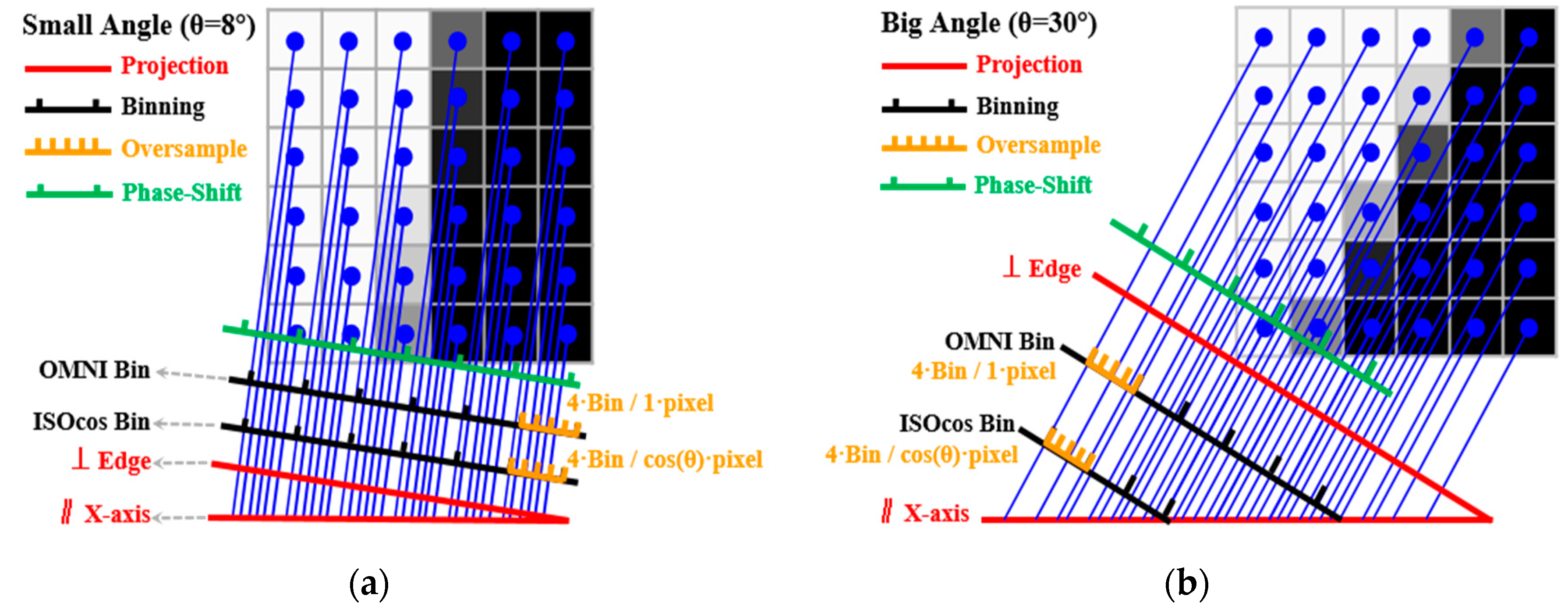
2.3. Analysis of Conventional Edge Method

The main steps of the existing modified edge methods derived from ISO 12233: 2017 [4] have not changed essentially, and they still include the following contents: ROI extraction, edge detection, ESF construction based on projection binning, LSF construction by difference or derivation, MTF calculation from Fourier transform and MTF compensation. Among these steps, the condition of the STAS edge greatly limits the practical application range of the edge method in the field of RS. If this constraint condition cannot be relaxed, the high-precision angle measuring model and ESF curve fitting model can hardly exert their effectiveness for those RS images lacking the STAS edge feature.

The ROI extraction and ESF construction step in the edge method correspond to the applicable limit of “straight edge” and “small tilt angle (STA),” respectively. This paper focuses on solving the STA application limitation for straight edges, that is, studying the conditions under which projection binning with arbitrary edge angle can be realized. For the “vertical edge”, there are two main projection schemes along the edge: projecting to the horizontal direction or the direction perpendicular to the edge. The two projection schemes are approximately the same when the edge angle is small. However, the two projection schemes cannot be approximated when the edge angle increases. ESF oversampling binning mainly includes two schemes based on unit pixel width (called OMNI binning [11]) or horizontal adjacent pixel projection path width (called ISO-cos binning [22]), both of which involve the determination of OSR and binning PS. A comparison of different schemes for projection and binning is shown in Figure 1. When adopting a fixed and same OSR (such as 4), the essential difference between ISO-cos and OMNI binning methods lies in whether the width of the bin changes with the edge angle. The bin width of ISO-cos is less than or equal to OMNI for arbitrary edge angle, which makes the possibility of the empty bin in OMNI less than ISO-cos under the condition of fixed OSR.

3. Analysis of Edge Method Accuracy

The principle of the edge method is not complicated, but its MTF measurement results often show low robustness and non-uniqueness. For example, it is difficult to keep the MTF results of the same edge image measured many times by the same algorithm completely consistent. The accuracy of the edge method is limited by the randomness of edge images used in different imaging fields and the strong coupling between algorithm steps. This section analyzes the main factors that affect the accuracy of the edge method: edge angle (Ang), oversampling rate (OSR), height and width of ROI (ROI-H and ROI-W), edge contrast (Con), random noise (noise level can be characterized by SNR) and gives suggestions on parameter determination with universal reference significance.

In this paper, four representative edge methods are used for simulation analysis: ISO 12233: 2017 international standard edge method [4], ISO-cos modified edge method [22], OMNI modified edge method [11], and OMNI-sin modified edge method with variable OSR [7], which are abbreviated as ISO, ISO-cos, OMNI, and OMNI-sin, respectively. In order to compare the accuracy of different modified edge methods, the non-critical analysis steps are unified: ROIs with the same shape, size, and position are determined, and the widely used row difference linear fitting method is used to detect the edge angle [4], the oversampled discrete ESF is differentiated to obtain LSF, and the same MTF compensation model is used [2]. The similarities and differences adopted in the main steps of the above methods are summarized in the following

Table 1. Projection and binning process comparison among four edge methods.

	Method	ISO 12233	ISO-cos	OMNI	OMNI-sin
Process
Project to		∥ X-axis	⊥ Edge	⊥ Edge	⊥ Edge
OSR		4	4	4	Variable OSR [7]
Bin Width (pixel)		1/4	cos(θ)/4	1/4	1/(Variable OSR)

:

Ideal discrete edge (IDE) image: The IDE image with specified size, angle, bright/dark gray values, and resolution can be simulated and generated by the heaviside function. It should be noted that the simulated IDE image contains the discrete sampling degradation only (i.e., $MT{F}_{IDE}\left(f\right)=$$MT{F}_{samp}\left(f\right)$), so $MT{F}_{IDE}\left(f\right)$ is slightly less than or equal to 1 in the whole SF ranges. The size of the simulated IDE image is 400 × 400 pixels, the resolution is 300 dpi, and the gray values of the bright and dark edges are 180 and 60, respectively. It should be noted that, in this paper, the reference value of $MT{F}_{samp}\left(f\right)$ for IDE images with different edge angles is approximately obtained by the mean value of MTF measurements of the above four edge methods.

Blurry degraded edge (BDE) image: The types and parameters of the blurry kernel do not affect the analysis of the edge method, so the Gaussian blurry kernel, which is the most widely used, with a size of 5 × 5 pixels, the mean value of 0 and the variance of 1 is determined. Based on the IDE image, the corresponding BDE image is obtained by convolution of 5×5 Gaussian blurry kernel. It should be noted that the simulated BDE image contains the discrete sampling degradation and blurring degradation (i.e., $MT{F}_{BDE}\left(f\right)=$$MT{F}_{samp}\left(f\right)\cdot MT{F}_{blur}\left(f\right)$). The theoretical value of $MT{F}_{blur}\left(f\right)$ can be calculated by the modulus of FFT of the Gaussian fuzzy kernel. The simulated partial BDE images with different edge angles of 0~45 deg are shown in Figure 2 (The simulated angle interval is 0.1 deg.).

Blurry degraded edge with different contrasts (BDE@Con): Based on the BDE image, eight kinds of BDE@Con edge images (0.04, 0.10, 0.15, 0.20, 0.36, 0.52, 0.68, 0.84) were obtained by adjusting the gray values of the bright (B) and dark (D) edges (B130/D120, B138/D112, B144/D106, B150/D100, B170/D80, B190/D60, B210/D40, B230/D20). The simulated partial BDE@Con images with different contrasts are shown in Figure 3.

Blurry, noisy degraded edge (BNDE) image: The added random noise is composed of Gaussian, uniform, exponential, and speckle noise which are common in actual RS images. In order to simplify the analysis model, the asymmetry of photon noise on both sides of the edge is not considered in this paper. Based on the BDE image, five kinds of SNR BNDE images (3.9, 4.2, 4.8, 10.0, 12.6) were obtained by adding noises with different intensities (See

Table 2. Noise parameter and SNR of different noise levels for different noise types.

	Noise Type	Gaussian Noise (Variance)	Uniform Noise (Threshold)	Exponential Noise (Mean)	Speckle Noise (Variance)	SNR (dB)
Noise Level
00 (noise free)		0.000	0	0	0.000	∞
01		0.001	1	1	0.001	12.6
02		0.005	2	2	0.005	10.0
03		0.010	3	3	0.010	4.8
04		0.015	4	4	0.015	4.2
05 (noise max)		0.020	5	5	0.020	3.9

below for detailed noise parameters.). The simulated partial BNDE images with different noise levels are shown in Figure 4.

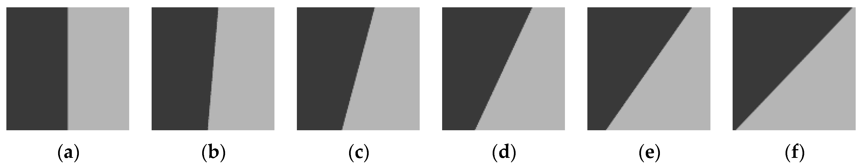
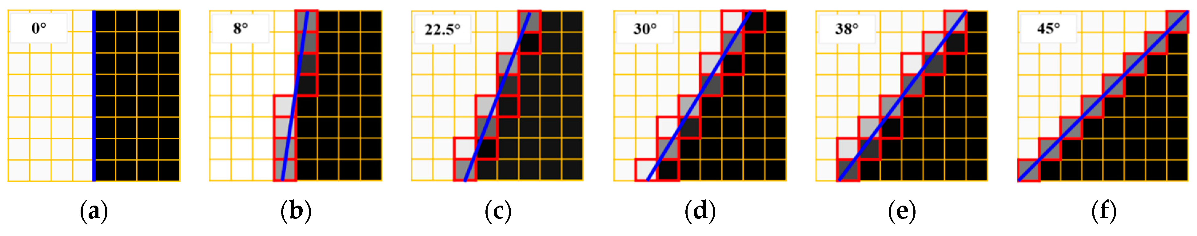
3.1. Edge Angle

If the absolutely vertical upward edge is taken as the reference of 0 deg and the clockwise is positive, the angle range of all possible edges is [0, 360] deg, which can be divided into the vertical edge (θ∈ [−45, 45] ∪ [135, 225] deg) and horizontal edge (θ∈ [45, 135] ∪ [225, 315] deg). According to the axisymmetric and centrosymmetric properties of edge features, and referring to the angle transformation equation of reference [7], [0, 360] deg edges can be correspondingly transformed into [0, 45] deg vertical edges for analysis. The angle transformation diagram is shown in Figure 5. In this section, four representative edge methods are used to measure the MTF of BDE images with different edge angles of 0~45 deg. The simulation results are expressed in Cartesian coordinates and polar coordinates, as shown in Figure 6.

Figure 6a–h show that the consistency of MTF curves obtained by [0.2, 14.5] deg edges is obviously higher than that of other angle interval edges in the whole frequency ranges. This conclusion is basically consistent with the view that accurate MTF measurement results can be obtained by [2,10] degree edge verified in literature [23]. It shows that MTF measurement with STA edges has high stability. When the edge angle is greater than 15 deg, the MTF curves appear a downward trend with the increase of edge angle in the middle and low frequency ranges (Roughly [0, 0.42] lp/pix). It can be clearly seen that the larger the angle is, the more obvious the MTF downward trend is. When the edge angle is greater than 30 deg, the MTF curves appear an upward trend with the increase of edge angle and tend to be aliased in the high frequency ranges (roughly [0.42, 0.50] lp/pix). The above simulation results further confirm the validity and rationality of ISO 12233′s recommendation of determining STA edges to measure MTF in horizontal or vertical directions approximately.

Figure 6e–h verify the effectiveness of measuring MTF in different directions with different angle edges. However, the simulation results show that when the edge images with the same blurry effect and different angles are used, the MTF results are different in various directions, which may be directly related to the rectangular grid structure of digital image detectors or displays. The physical structure leads to different sampling degradation in different directions. The blurry degradation effect of simulated edge images with different angles is consistent, but the sampling degradation effect is different, so the actual MTF curves are scattered with the change of edge angles. The schematic diagrams of degradation caused by a digital sampling of edge images from different angles are shown in Figure 7. In particular, the conclusion is reasonable speculation, and it is necessary and valuable to further study and verify.

The smoothness and convergence of MTF curves in the middle and high frequency ranges in Figure 6a,b,e,f, which adopt ISO-cos projection binning, are obviously better than those in Figure 6c,d,g,h, which adopt OMNI projection binning. It indirectly verifies that the accuracy of the ISO-cos projection binning scheme is better than that of OMNI, which is consistent with the graphical analysis result of Figure 1. The binning principles of ISO-cos and OMNI, both of which adopt fixed OSR = 4, are essentially different: the oversampled bin width of ISO-cos (cos(θ)/4 (pix)) is always less than or equal to that of OMNI (1/4 (pix)) for arbitrary edge angle. To sum up, the binning adaptability of ISO-cos is better than that of OMNI. OMNI binning aims to reduce the probability of an empty bin for large-angle edge projection, while ISO-cos binning aims to achieve more accurate binning.

All in all, the feasibility of multidirectional MTF measurements based on arbitrary angle edges can improve the practical application efficiency of the edge method. For the edges in different angle intervals, we can adopt the ISO-cos projection binning model and a more adaptive OSR model to improve the effectiveness and accuracy of the edge method.

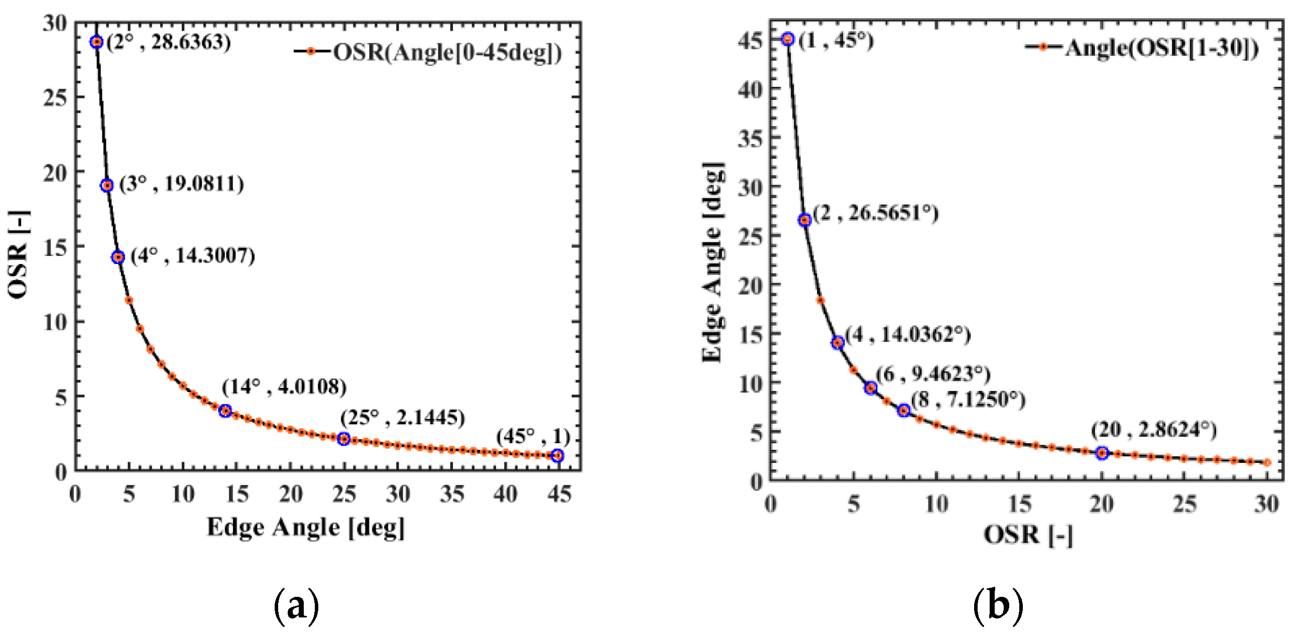
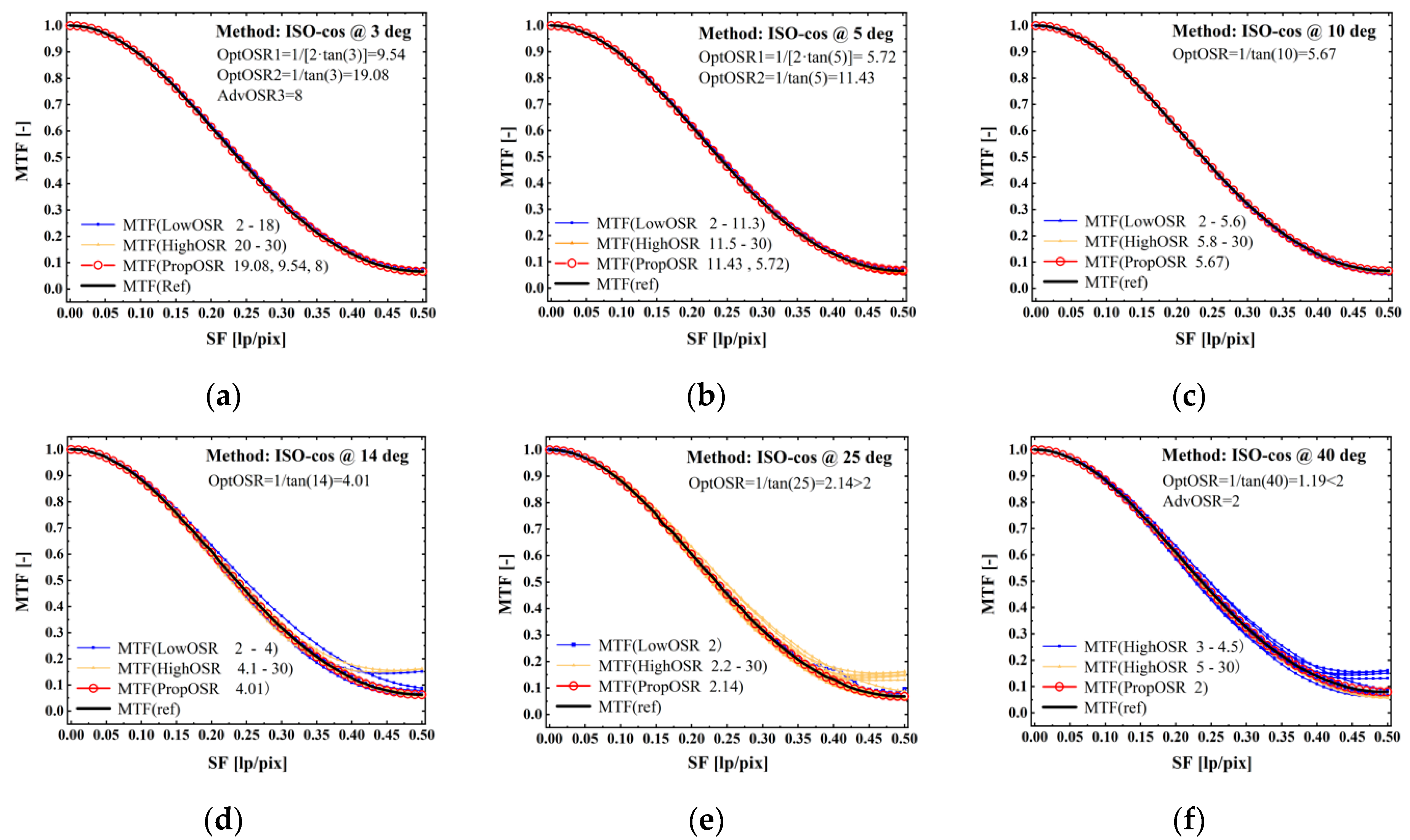
3.2. Oversampling Ratio

Binning, OSR, and phase shift (PS) play a decisive role in the accuracy of ESF construction. Adopting 4× OSR has the advantages of moderate calculation and obtaining valid data before the cut-off frequency, but it may not be suitable for edges with a too-small or too-large angle. Related research [7] proves that the accuracy of the edge method can be further improved by adopting different OSRs for different edge angles, so it is necessary to propose a more adaptable OSR model.

The row and column projection path distance formed by projecting the row and column pixels of ROI along the edge to the direction perpendicular to the edge plays an important role in the reasonable determination of OSR. For [0, 45] deg vertical edge, the projection path distance of adjacent pixels in each row (or adjacent columns) is cos(θ)(pix), and the projection path distance of adjacent pixels in each column (or adjacent rows) is sin(θ)(pix). Based on the ISO-cos binning strategy, it is necessary to bin multi-row projection data with a projection pitch of sin(θ)(pix) that fall within the width of cos(θ)(pix). The optimal adaptive binning of the projection pixels can be realized when the OSR is determined as 1/tan(θ) = (cos(θ)/sin(θ)). Figure 8 shows a comparative schematic diagram of the ISO-cos binning process when different OSRs are determined for different edge angles. It can be seen that 1/tan(θ) determines the minimum number of effective rows to be determined and the optimal OSR for adaptive binning. When the actual OSR is higher than the optimal OSR, there will be empty bins, while when it is lower than the optimal OSR, the data utilization rate will be insufficient. The relationship between the ideal OSR and edge angle is shown in Figure 9. When the edge angle is less than 3 deg, the minimum effective rows and ideal OSR are greater than 20 and increase sharply with the decrease of the edge angle. When the edge angle is greater than 25.56 deg, the minimum effective rows and ideal OSR are less than 2 and gradually decrease to 1 with the increase of edge angle. The practical application of the edge method requires that the OSR should not be too high or too low. OSR higher than 10 will obviously increase the calculation cost, but the accuracy will not be improved qualitatively. Meanwhile, an OSR lower than 2 will decrease the accuracy and make it difficult to obtain MTF accurately before Nyquist frequency.

In this section, the ISO-cos edge method is used to measure the MTF of BDE images with 3, 5, 10, 14, 25, and 40 deg, and three kinds of OSR, ideal, low, and high, are used to simulate and verify the influence of different OSR on the accuracy of edge method. 1/tan(θ) is used to calculate the ideal optimal OSR (OptOSR/OptOSR2) corresponding to different edge angles. When the ideal OSR is greater than 8, the ideal suboptimal OSR (OptOSR1) will be calculated by 1/[2·tan(θ)], and when the suboptimal OSR is still greater than 8, 8 will be determined as the advised OSR (AdvOSR3). When the ideal OSR (OptOSR1) is less than 2, 2 will be determined as the advised oversampling rate (AdvOSR), and the problem of an empty bin will be solved by interpolation. It should be noted that the MTF reference value MTF(Ref) of the BDE image is calculated by $MT{F}_{samp}\left(f\right)\cdot MT{F}_{blur}\left(f\right)$ (for the methods of obtaining $MT{F}_{samp}\left(f\right)$ and $MT{F}_{blur}\left(f\right)$, see the previous description in Section 3). The simulation results are shown in Figure 10.

Figure 10a–f shows that when the ideal optimal or suboptimal OSR calculated based on 1/[k∙tan(θ)] (k∈Z₊) is determined for arbitrary angle edge of [0, 45] deg, the edge method accuracy is higher than that of other higher or lower OSR. The consistency of MTF curves with different OSRs in Figure 10a–c is higher than in Figure 10d–f. On the one hand, it indicates that OSR has little influence on STA edges (e.g., ≤10 deg), which is related to the tight projection path with more data involved in binning and less possibility of an empty bin. On the other hand, it indicates that OSR greatly influences the large angle edges (e.g., ≥14 deg) when the higher or lower OSR is used, which is related to the sparse projection path with fewer data involved in binning and the greater possibility of the empty bin.

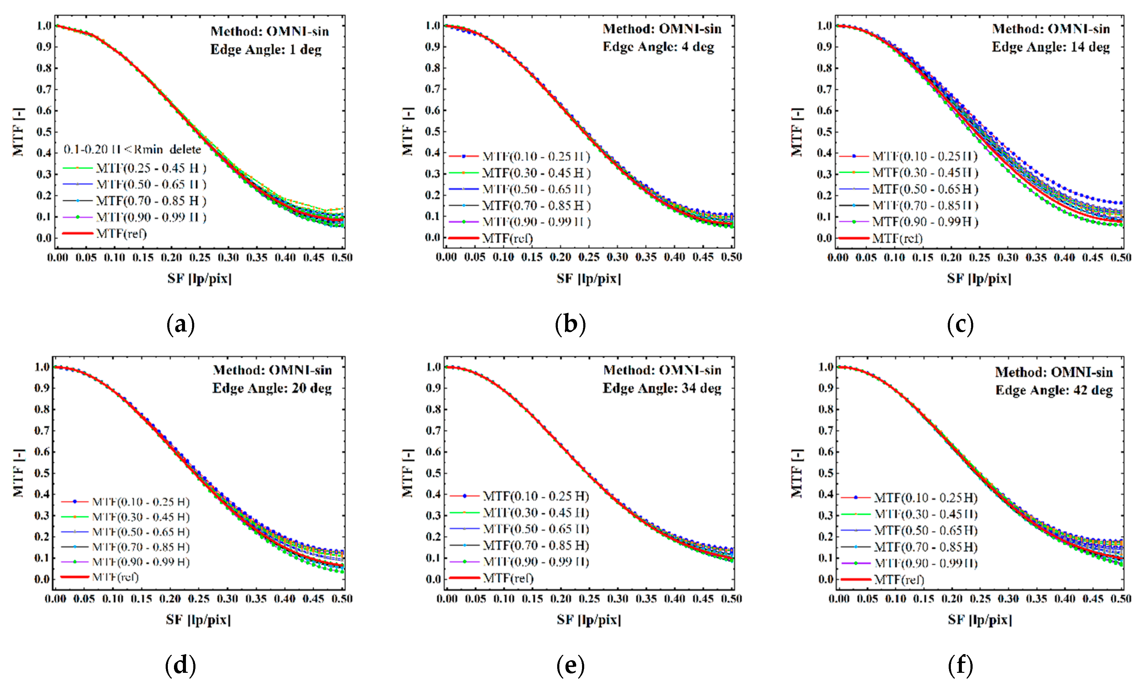
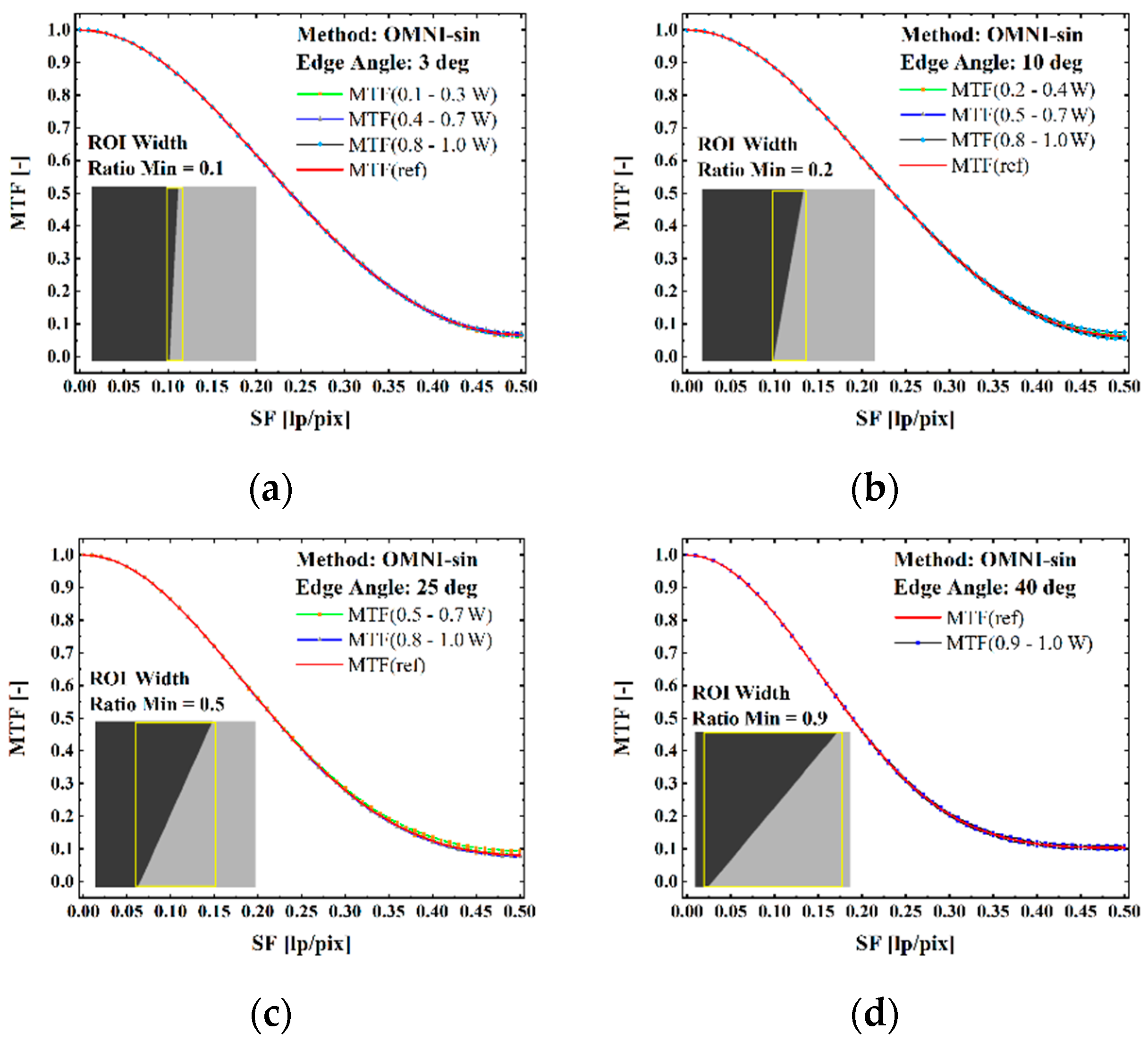
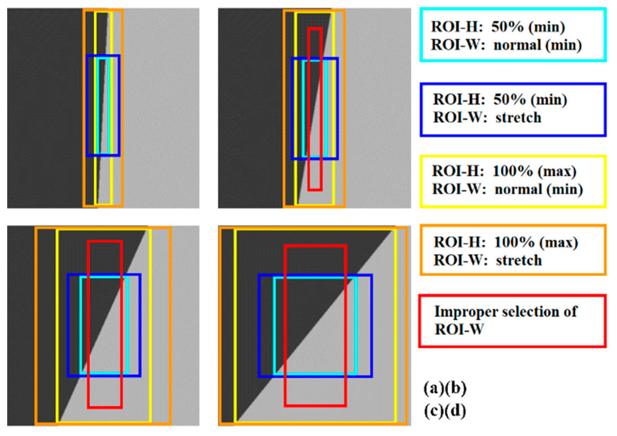
3.3. Region of Interest (ROI)

It is generally believed that the ROI extraction in edge method should ensure the vertical or horizontal edge intersect with the upper-lower sides or the left-right sides of the ROI, respectively, but the position and size of ROI are not considered. In practice, it is found that even when the same edge method is used to measure the same edge image, the MTF results may differ with the size and position of the determined rectangular ROI, which will lead to a lack of robustness. It is necessary to study the accurate constraint conditions of ROI extraction to realize automatic and effective ROI extraction. References [11,14] verify that extracting any irregular ROI shape with edges does not affect the accuracy of the edge method, thus relaxing the constraint of ROI shape. However, it is more difficult to extract any irregular shape than a rectangle, and the result of irregular extraction is difficult to process, which leads to its limited practicability. Considering the practicality and convenience of data processing, this section still adopts rectangular ROI extraction.

According to the analysis results in Section 3.1 and Section 3.2, it is necessary to consider the concept of “the minimum number of effective rows” (R_min = 1/tan(θ)) to meet the oversampled binning requirements of edge projection at different angles in order to avoid the empty bin caused by insufficient ROI extraction data. However, in order to ensure the accuracy of the edge method, the height of the actual extracted ROI is usually a multiple of R_min. This section mainly analyzes the influence of ROI size, including height (ROI-H) and width (ROI-W) of ROI, on the accuracy of the edge method and provides quantitative suggestions for efficient ROI extraction. In order to analyze the influence of ROI size on the edge method more accurately, the ROI extraction position is determined in the center of the edge image, and the ROI with a specified size is automatically extracted by programming. Since the relevant influencing factors of the edge method have nothing to do with which the improved method is adopted, this section will adopt another improved edge method, OMNI-sin, for fairness. When analyzing the influence of ROI-H, the ratio of ROI-H to the height of the edge image is determined as 0.1~0.99, and the ROI-W is automatically determined according to the intersection of the edge and the upper-lower sides, which extend 5 pixels to both sides, respectively. When analyzing the influence of ROI-W, ensure the same ROI-H, and control the extraction of different ROI-W by the ratio of pixel width extending to both sides to edge image width. In this section, the ROI-H factor is analyzed for 0~45 deg BDE edges (at an interval of 0.5 deg). The measurement results representing different angle types are randomly determined and shown in Figure 11. The simulation results of the influence of ROI-W on the accuracy of the edge method are shown in Figure 12. The MTF(Ref) of the BDE image is as described in Section 3.2.

The MTF curves in Figure 11a–f show various intensity divergences in the middle and high frequency, and the higher the frequency, the more obvious the divergence. It proves that the ROI-H has an influence on the accuracy of the edge method. Furthermore, it can be founded that the consistency and accuracy of MTF are relatively higher when the ratio of ROI-H to edge image height is greater than 0.5. The MTF curves in Figure 12a–d show high consistency in all frequency ranges. On the premise of satisfying the minimum width, even if the ROI-W is further increased, the improvement of MTF accuracy will be limited, and the computational cost will be increased. When the uniformity of image quality is poor, the MTFs of different edge regions fluctuate greatly. Multi-MTF measurement can be carried out for multi-regions and multi-ROI-H. The schematic diagram of effective and invalid ROI extraction is shown in Figure 13.

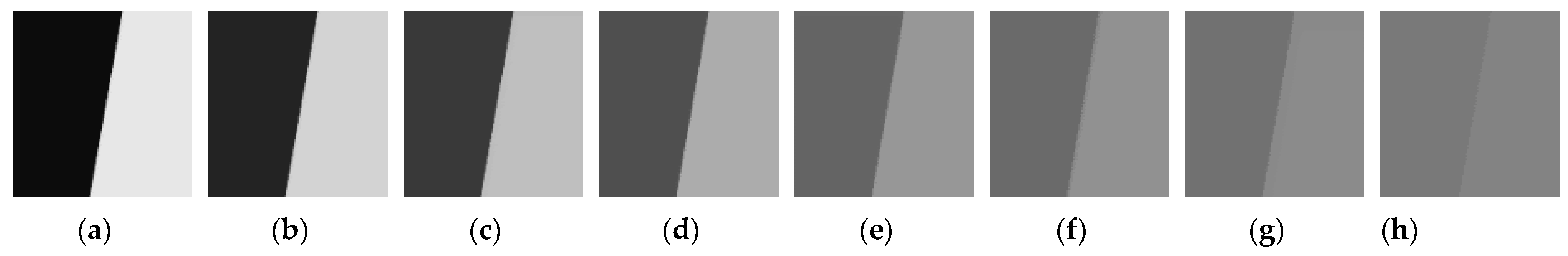
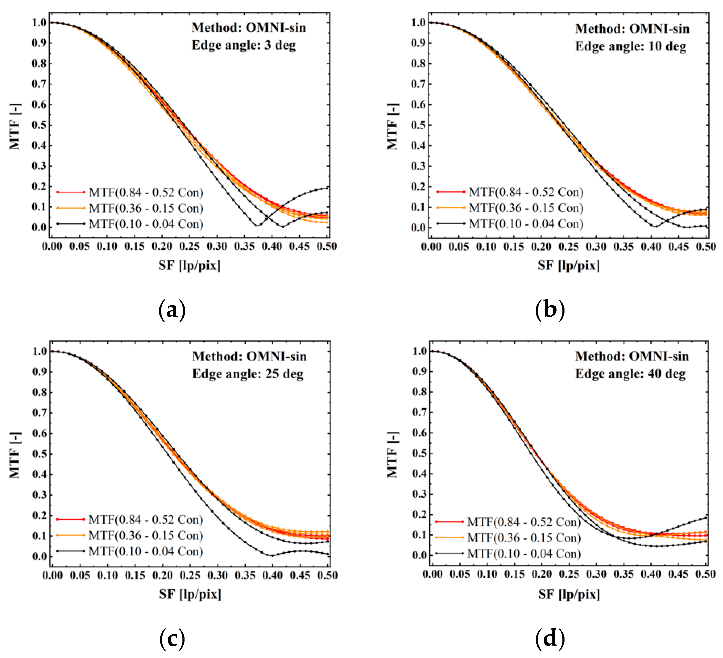
3.4. Edge Contrast

Generally, related studies have proved that contrast does not affect the accuracy of MTF measurement by edge method [10]. However, when the edge contrast is too low, that is, it is difficult to distinguish the edge visually, and the stability of MTF measurement results will also be affected. Therefore, in this section, contrast is analyzed again as an influencing factor. The BDE images with four angles of 3, 10, 25, and 40 deg, 400 × 400 pixels, and 300 dpi are determined for analysis, and the edge contrast is controlled at 0.04~0.84 by adjusting the gray values on both sides of the edge. The OMNI-sin edge method is used to measure the MTF of the edge images with different angles and different contrasts in Figure 3, and the simulation results are shown in Figure 14.

Figure 14a–d show that the accuracy of the edge method is improved with the increase of edge contrast, but the improvement effect is not obvious. The consistency of MTF curves with edge contrast greater than 0.15 is relatively high, which indicates that the contrast has little influence on the accuracy of the edge method. It is consistent with the conclusion in reference [10] and the consensus in the field of MTF measurement. However, when edge contrast is lower than 0.1, MTF in the middle and high frequency ranges is prone to aliasing. This paper only determines that too low edge contrast will have a certain impact on the stability of MTF measurement. It is necessary to further analyze and verify to what extent the contrast reduction will seriously affect the accuracy of the edge method.

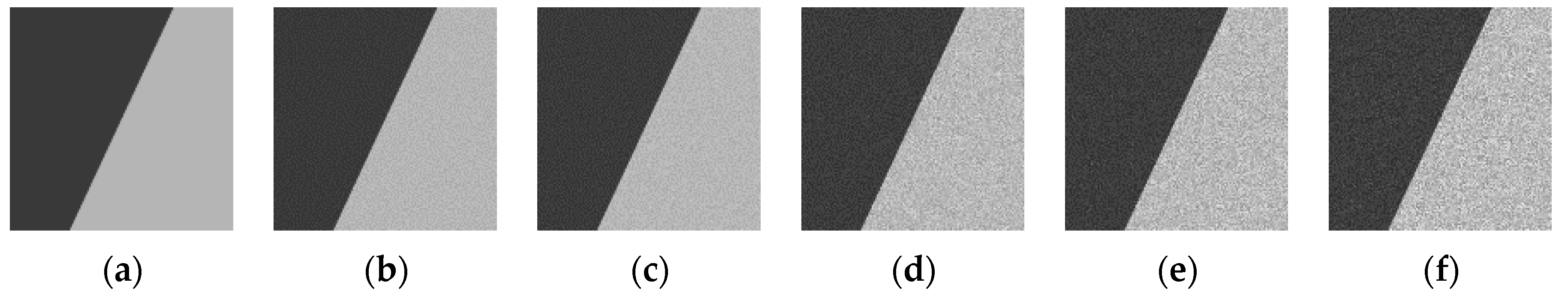
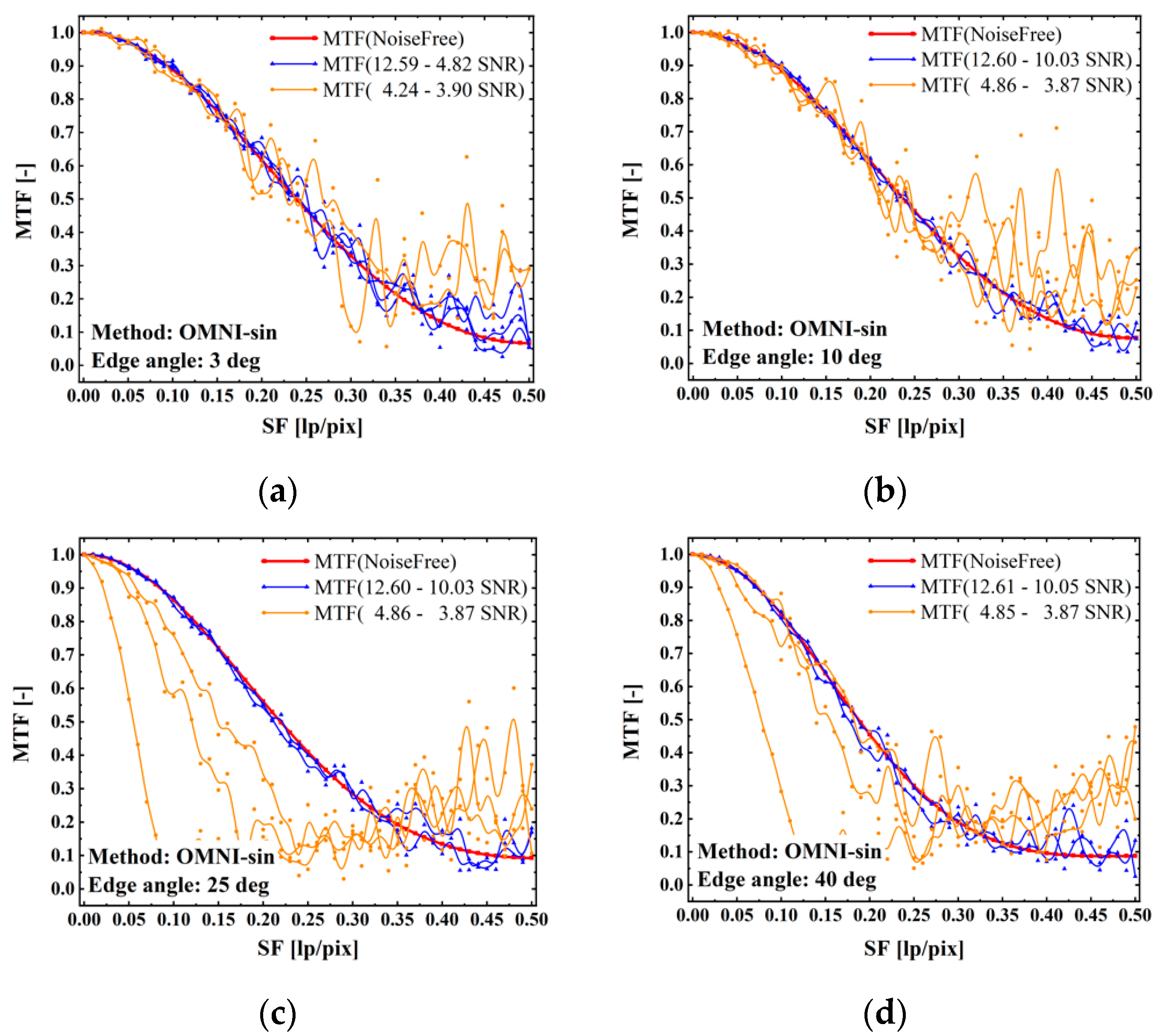
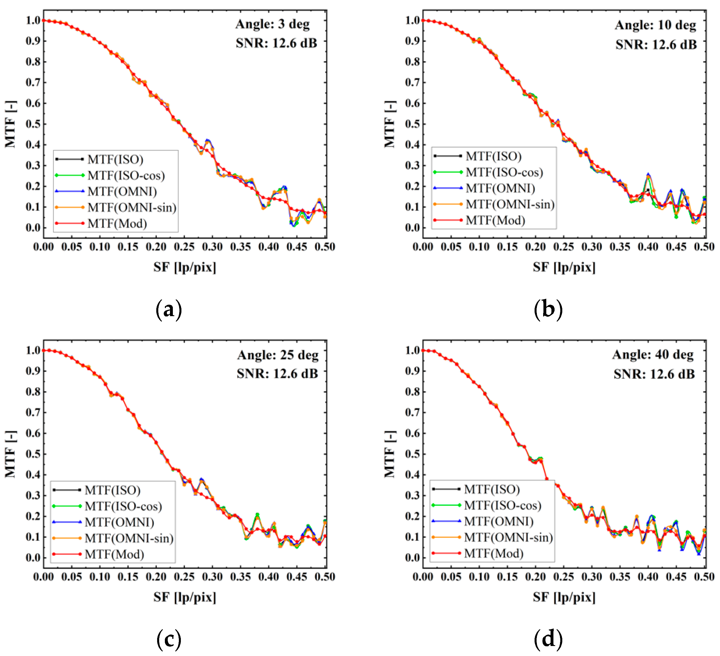
3.5. Random Noise

In this section, Gaussian, gamma, uniform, and speckle noise, which are four typical noises, are mixed and added into ideal edge images as noise simulation sources in RS images. Different noise levels are controlled by modifying the variance and mean of noise. Moreover, the parameters of added noise are shown in Table 2. The BNDE images with four angles of 3, 10, 25, and 40 deg, 400 × 400 pixels, and 300 dpi are determined for analysis, and the SNR of edge images is controlled to be 3.9~12.6 dB by adjusting different noise parameters. The OMNI-sin edge method is used to measure the MTF of edge images with different angles and different SNRs in Figure 4, and the simulation results are shown in Figure 15.

Figure 15a–d shows that MTF curves will fluctuate to some extent as long as there is noise in the edge image. When the SNR of the edge image is greater than 10 dB, both the noisy fluctuant MTF and the noiseless smooth MTF still have high consistency, and the measured results are still valid. When the SNR of the edge image is lower than 4.8 dB, the possibility of aliased MTF is greatly increased. In this case, MTF deviates from the trend line of noiseless MTF in all frequency ranges, so the confidence of the measured MTF is extraordinarily low. The larger the edge angle, the more obvious the influence of noise. In this study, only the upper and lower limits of two thresholds are preliminarily determined, but the influence of the signal-to-noise ratio between 4.8 and 10 dB needs further study.

4. Practical Multidirectional MTF Measurement Method

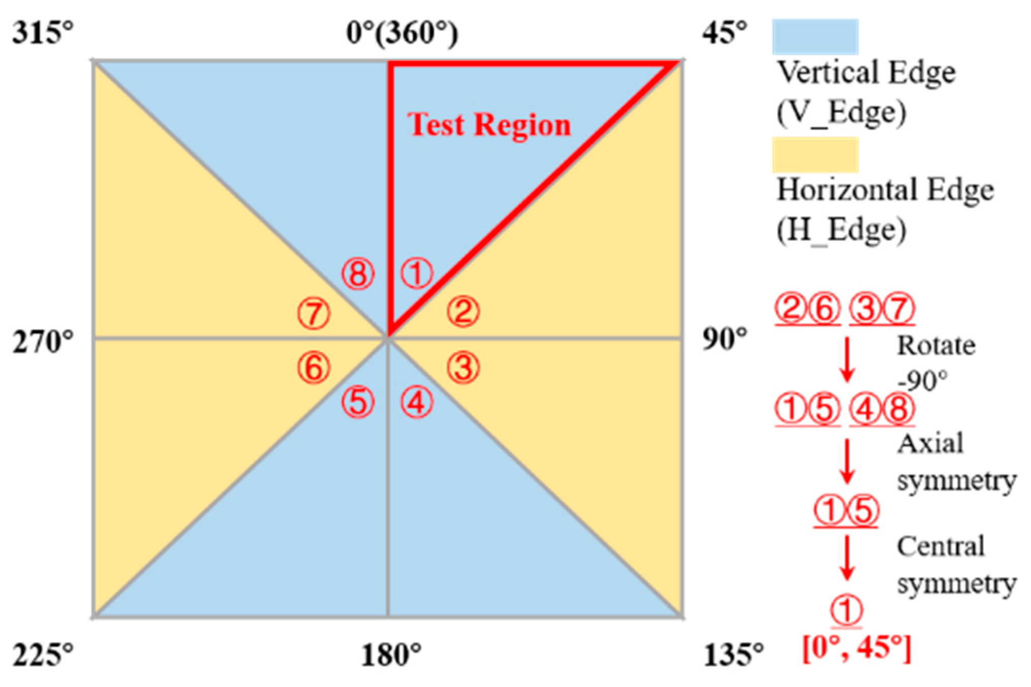
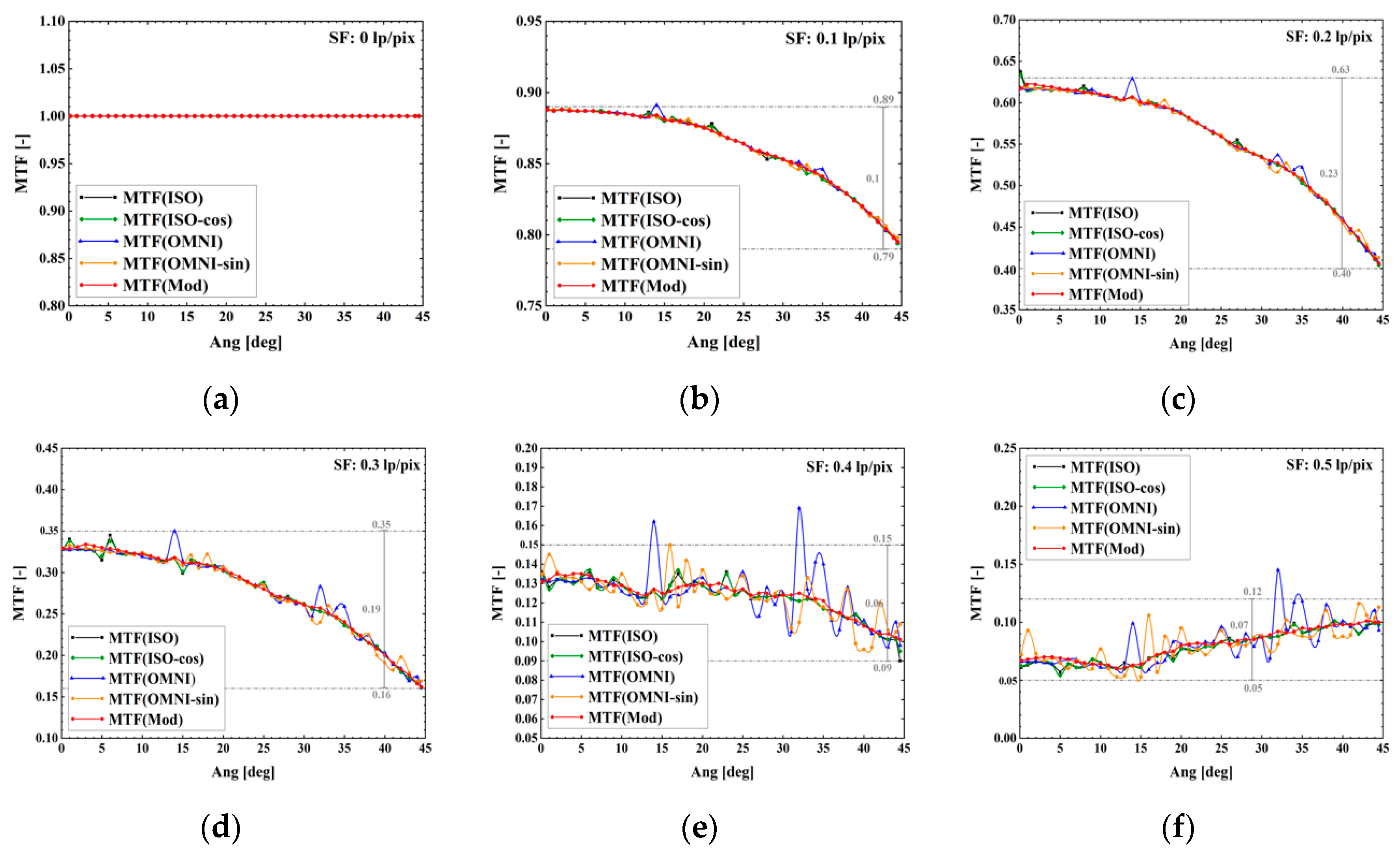
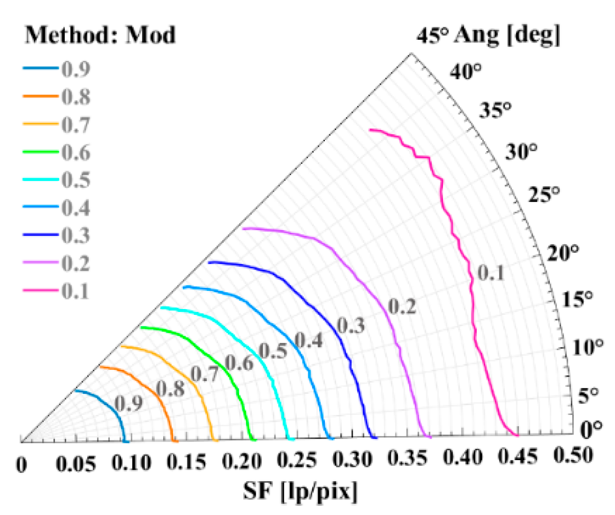
4.1. Rationality of Multidirectional MTF

Based on the analysis conclusion in Section 3.1, it can be seen that the results of measuring MTF in the horizontal or vertical direction with 0~14.5 deg edge are effective and reliable. If multidirectional MTF needs to be measured, the edge ROI should be projected in the direction perpendicular to the edge. The effectiveness of multidirectional MTF measurement will make the application of the edge method no longer limited by STA edge. The MTF measured by a certain angle edge can further reflect the image quality degradation of the sampling imaging system in the whole field of view, but it needs a more reasonable sampling MTF compensation model. In addition, PSF parameters obtained by multidirectional MTF can be used for non-blind image restoration.

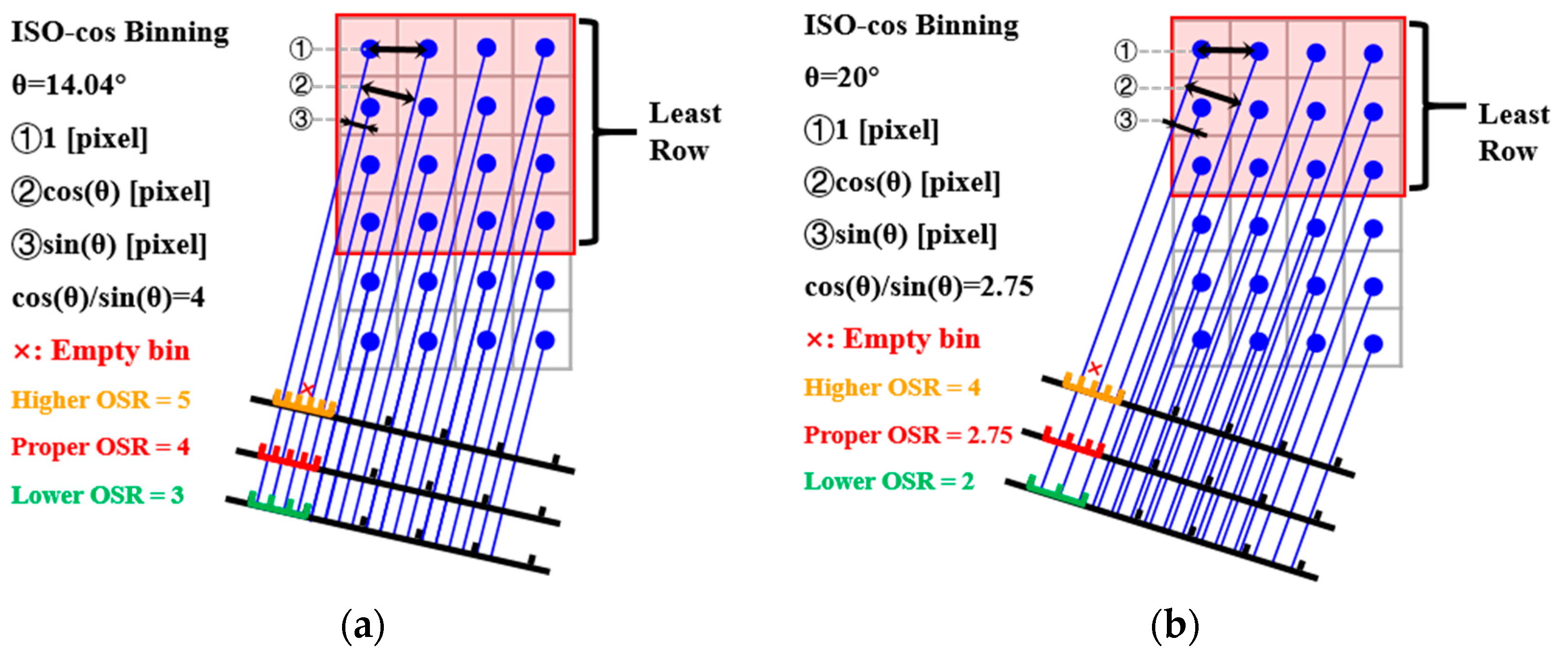
4.2. Modified Adaptive OSR Model

Based on the analysis conclusion in Section 3.2, this paper proposes an OSR determination model which is more in line with the principle of multidirectional projection and the actual calculation demand, as shown in Equation (13).

$$OSR=\left\{\begin{array}{cc}8& ,\theta \in [0,3.18)\hspace{1em}or\left[0,\arctan \left(\frac{1}{18}\right)\right)\mathrm{deg}\\ \frac{1}{2\cdot \tan (\theta )}& ,\theta \in [3.18,6.34)\hspace{1em}or\left.\left[\arctan \left(\frac{1}{18}\right),\arctan \left(\frac{1}{9}\right)\right.\right)\mathrm{deg}\\ \frac{1}{\tan (\theta )}& ,\theta \in [6.34,14.04]\hspace{1em}or\left[\arctan \left(\frac{1}{9}\right),\arctan \left(\frac{1}{4}\right)\right]\mathrm{deg}\\ \max \left[{\frac{1}{\tan (\theta )}}_{}{,}_{}2\right]& ,\theta \in (14.04,45]\hspace{1em}or\left.\left(\arctan \left(\frac{1}{4}\right),\arctan \left(1\right)\right.\right]\mathrm{deg}\end{array}\right.$$

(13)

When θ∈[0, 3.18) deg, the edge angle is “too small,” and the projection path is too dense. The ideal optimal OSR in this angle interval is all greater than 18. The minimum effective number of ROI rows (R_min = 1/tan(θ)) corresponding to the small angle edge is relatively large. If the ideal high OSR is still adopted, the calculation cost will be increased, and the accuracy will not be improved obviously. Therefore, considering the accuracy and calculation cost of MTF measurement for small angle edges, the OSR is determined as 8, which can sufficiently ensure the accuracy of the edge method.

When θ∈[3.18, 6.34) deg, the edge angle is “relatively small,” and the projection path is still relatively dense. The ideal optimal OSR in this angle interval lies between (9, 18]. If the ideal OSR in this interval is all reduced by 0.5 times, the OSR will be between (4.5, 9], which is moderate and conforms to the ideal suboptimal OSR model 1/[k∙tan(θ)] (k∈Z₊). Therefore, the actual OSR will be determined according to the ideal suboptimal OSR model 1/[2∙tan (θ)].

When θ∈[6.34, 14.04] deg, the edge angle is “moderate,” and the projection path distance is moderate. The ideal OSR of this angle interval is moderate, which lies between [4,9] and meets the actual needs of engineering. Therefore, the actual OSR will be determined according to the ideal optimal OSR model 1/tan(θ).

When θ∈(14.04, 45] deg, the edge angle is “too big,” and the projection path is sparse. The ideal optimal OSR corresponding to this angle interval is small, lies between [1, 4), which shows the projection data used for ESF construction is insufficient. In order to obtain the MTF before Nyquist frequency (0.5 lp/pix) accurately, the actual OSR should be above 2. When the ideal optimal OSR is less than 2, the actual OSR is determined as 2, and the empty bin in the construction of oversampled ESF can be filled with the vacant value by linear interpolation. When the ideal optimal OSR is greater than or equal to 2, the actual OSR will be determined according to the ideal optimal OSR model 1/tan(θ). Therefore, the actual OSR will be determined according to the max[1/tan(θ), 2] model to ensure that the OSR is greater than or equal to 2.

4.3. Multi-state MTF Measurement

In order to reduce the fluctuation of MTF results caused by different ROI extraction, this paper will measure MTF several times by extracting different ROI-H and different positions in the same edge image and improve the accuracy of the edge method from the statistical point of view. The multi-ROI automatic extraction strategy proposed in this paper is shown in Algorithm 1. When the determined edge image size is large enough, the multi-ROI will be automatically extracted according to the condition that X_max-R_min > 10, and ten sub-ROIs with different sizes and positions will be extracted. R_min represents the least number of valid rows. X_max-R_min represents the maximal number of valid row areas. The specific calculation formula is shown in Algorithm 1. According to the analysis results in Section 3.3, when the ROI-H ratio is above 0.5, the robustness of MTF results is relatively high. Therefore, only six extracted sub-ROIs with an ROI-H ratio of 0.5~1: ROI5~ROI10 can be used in practical application.

ISO-cos projection binning is adopted in the modified edge method. In order to further improve the accuracy, multi-phase binning is adopted as an auxiliary method (see Figure 1 for the schematic diagram of binning PS). For the specific application diagram of a multi-phase binning method, please refer to reference [15]. In this paper, the number of binning PS (PS_Num) is adaptively determined according to the edge angle as Equation (14). When the edge angle is “too small,” the projection data is the largest. It is not suitable for the ideal optimal OSR model, so the binning PS is set to the maximum (such as 8) to ensure the accuracy. When the edge angle is “moderate,” the stability and accuracy of the edge method are high, so the number of binning PS is set to a minimum (such as 4) to save the computational cost. When the edge angle is “relatively small or large”, the accuracy of the edge method is average, so the number of binning PS is set moderately (such as 6).

Algorithm 1 Automatic determination strategy of multi-ROI for edge image

Input: ①Edge image, ②Edge angle(θ), ③Number of edge image row(R).

Calculation: ①Least number of valid rows (Rmin = ceil(1/tan(θ))),

②Maximal number of valid row area (Xmax-Rmin = floor(R/Rmin)).

where ROI Height is k·Full or g·Rmin (k∈(0,1], g∈Z+);

where ROI Position should be determined from Top, Middle or Bottom.

if Xmax-Rmin∈(0,3)

ROI-Num = 1→ROI1(Full, Middle)

elseif Xmax-Rmin∈[3,5)

ROI-Num = 4→ROI1(3·Rmin, Top), ROI2(3·Rmin, Middle), ROI3(3·Rmin, Bottom),

ROI4(Full, Middle).

elseif Xmax-Rmin∈[5,10)

ROI-Num = 8→ROI1(3·Rmin, Top), ROI2(3·Rmin, Bottom), ROI3(5·Rmin, Middle),

ROI4(5·Rmin, Top), ROI5(5·Rmin, Bottom), ROI6(0.5·Full, Top),

ROI7(0.5·Full, Bottom), ROI8(Full, Middle).

else Xmax-Rmin> 10

ROI-Num = 10→ROI1(3·Rmin, Top), ROI2(5·Rmin, Bottom), ROI3(8·Rmin, Middle),

ROI4(10·Rmin, Middle), ROI5(0.5·Full, Top), ROI6(0.6·Full, Middle),

ROI7(0.7·Full, Bottom), ROI8(0.8·Full, Top), ROI9(0.9·Full, Bottom),

ROI10(Full, Middle).

end

$$PS\_Num=\left\{\begin{array}{cc}8& ,\theta \in [0,3.18)\hspace{1em}or\left[0,\arctan \left(\frac{1}{18}\right)\right)\mathrm{deg}\\ 6& ,\theta \in [3.18,6.34)\hspace{1em}or\left.\left[\arctan \left(\frac{1}{18}\right),\arctan \left(\frac{1}{9}\right)\right.\right)\mathrm{deg}\\ 4& ,\theta \in [6.34,14.04]\hspace{1em}or\left[\arctan \left(\frac{1}{9}\right),\arctan \left(\frac{1}{4}\right)\right]\mathrm{deg}\\ 6& ,\theta \in (14.04,45]\hspace{1em}or\left.\left(\arctan \left(\frac{1}{4}\right),\arctan \left(1\right)\right.\right]\mathrm{deg}\end{array}\right.$$

(14)

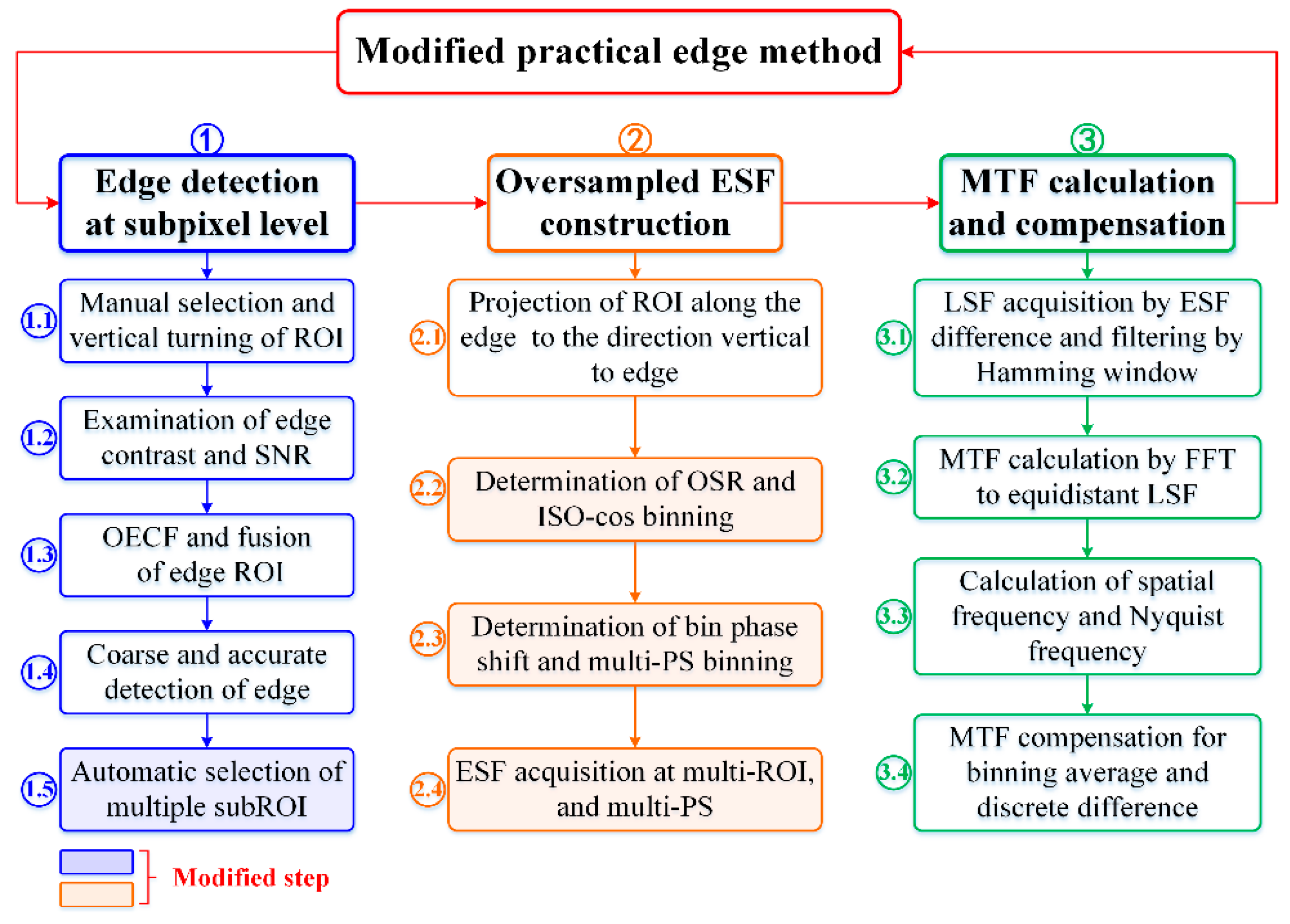
4.4. Modified Practical Edge Method

Based on the modified strategies in 4.1~4.3, this paper proposes a practical multidirectional MTF modified edge method with an adaptive determination of OSR. The flow chart of the modified practical edge method is shown in Figure 16.

The subpixel edge detection process is explained as follows: the actual image may not only contain edge features, so step 1.1 is to preliminarily extract the vertical or horizontal edge ROI from the actual image with edges. In order to facilitate the computation and processing, the horizontal edge should be rotated into the vertical edge. Step 1.2 is used to verify whether the extracted edge contrast (which should be greater than 0.1) and edge SNR (which should be greater than 10 dB) can guarantee the accuracy and validity of MTF measurement results. Step 1.3 is used to selectively perform inverse photoelectric conversion on actual images and multi-layer data fusion of color images. In step 1.4, the accuracy of edge angle determined by coarse and fine edge detection twice can meet the MTF measurement requirements in most imaging fields. Both coarse and fine edge detection are composed of three steps: filtering each row of ROI data, determining edge points by row difference, and performing least square linear fitting on edge points. The difference between the coarse and fine edge detection lies in the application of a symmetric Hamming window filter and an asymmetric Hamming window filter based on coarse positioning edge points. In step 1.5, firstly, calculate the minimum number of rows R_min(=1/tan(θ)) of effective ROI according to the edge angle, then calculate the maximum number X_max-R_min(=R/R_min) of optional R_min according to the number of rows R of input edge ROI, and finally, extract multiple sub-ROIs with different sizes and different positions that meet the MTF measurement requirements according to the multi-ROI automatic extraction algorithm in Algorithm 1.

The modified practical edge method in this paper constructs multiple ESF by automatically extracting multiple ROI and binning with multiple PS. In step 2.1, each ROI is projected along the edge to the direction perpendicular to the edge, and multidirectional projection data is obtained. In step 2.2, the OSR with stronger adaptability is determined by the variable OSR determination model proposed in Section 4.2, and the oversampled ESF is constructed according to ISO-cos binning scheme. In step 2.3, the number of binning PS is determined according to the model mentioned in Section 4.3, and the accuracy of the edge method is improved by constructing multi-PS oversampled ESF. To sum up, a plurality of ESFs will be obtained from multiple measurement states, i.e., multiple ROIs and multiple binning phases.

It is found that the calculation rationality of spatial frequency (SF) and the accuracy of the correspondence between SF and MTF directly determine the accuracy and reliability of the edge method, but the relevant research shows little about the accurate calculation of SF. The calculation of SF and Nyquist frequency depends on edge image resolution DPI (e.g., 300 dpi), edge angle θ (e.g., 10 deg), the number of discrete LSF point L (even number) participating in FFT, and OSR (e.g., 1/tan(10) = 5.67). Assume that the pixel spacing of the edge image is del (mm), the projection path spacing of adjacent pixels in each row is delcorr, the Nyquist frequency is freNyq, the number of valid data after FFT is Num, and the spatial frequency value to be calculated is SF. The SF and freNyq are calculated and deduced as follows:

$$\begin{array}{l}del=\frac{25.4}{DPI}\left(\mathrm{mm}\right)\hspace{1em}delcorr=del\cdot \cos \left(\theta \right)\\ freNyq=0.5\cdot \frac{1}{delcorr}\left(\mathrm{lp}/\mathrm{mm}\right)\hspace{1em}or\hspace{1em}0.5\left(\mathrm{lp}/\mathrm{pix}\right)\\ Num=\frac{L}{2}\\ SF=OSR\cdot \frac{\left[0:\left(Num-1\right)\right]}{L}\cdot \frac{1}{delcorr}\left(\mathrm{lp}/\mathrm{mm}\right)\hspace{1em}or\hspace{1em}OSR\cdot \frac{\left[0:\left(Num-1\right)\right]}{L}\left(\mathrm{lp}/\mathrm{pix}\right)\end{array}$$

(15)

The main differences between the modified method (named Mod) and other edge methods are different ROI extraction strategies, different OSR determination models, and different ESF binning PS schemes.

5. Comparative Experiments and Discussion

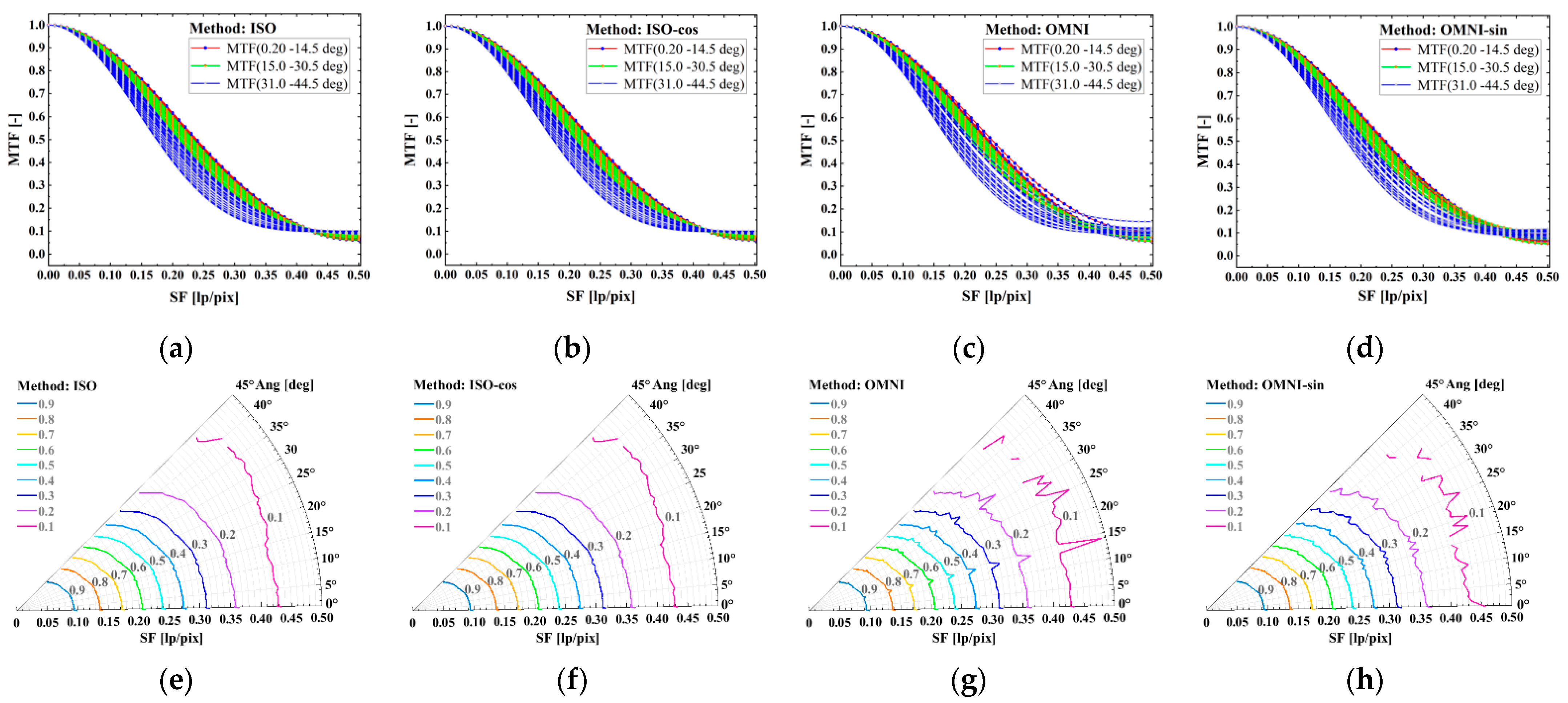
5.1. Simulation: Proposed Method vs. Other Methods

The Mod edge method is compared with the four representative edge methods used in the previous simulation analysis. The 0~45 deg BDE images are used for testing, and the MTF results of five methods at 0, 0.1, 0.2, 0.3, 0.4, and 0.5 lp/pix are compared. The simulation results are shown in Figure 17.

It can be seen from Figure 17a–f that the robustness of Mod, ISO, and ISO-cos edge methods in all frequency ranges is better than that of OMNI and OMNI-sin edge methods. However, the performance superiority of Mod is not obvious compared with ISO-cos because the test image is noiseless and the image quality uniformity in different areas is high. On the premise of ensuring the accuracy of MTF measurement, the Mod edge method mainly solves the problem of weak robustness caused by the complicated image quality. In addition, it can be clearly observed from Figure 17 that the data volatility of MTF results measured by the OMNI edge method is the greatest; that is, the possibility of abnormal measured values is the greatest. This also indirectly verifies the analysis conclusion in the second paragraph of Section 2.3 and Figure 1; that is, the accuracy of ISO-cos projection binning strategy is superior to OMNI projection binning strategy in principle. However, the data volatility of OMNI-sin measurement results is lower than that of the OMNI method because the variable OSR model with stronger adaptability improves the stability of MTF measurement to some extent.

Referring to the simulation process in Figure 6e–h, the simulation results according to the Mod edge method are shown in Figure 18. Comparing the smoothness and continuity of the polar coordinate curves of Figure 18 and Figure 6e–h, it can be seen that the multidirectional MTF measurement of the Mod edge method is more robust.

The analysis in Section 3.5 shows that when the SNR of the edge image is greater than 10 dB, the MTF result is reliable. Therefore, in order to further verify the performance of the Mod edge method, the simulated BNDE image with an SNR of 12.6 dB is used for MTF measurement, and the simulation result is shown in Figure 19.

It can be seen from Figure 19a–d that when there is noise in the image, the MTF measurement robustness of the Mod edge method in the whole frequency ranges is higher than that of ISO, ISO-cos, OMNI, and OMNI-sin edge methods, especially in the high frequency ranges, which proves that Mod edge method has certain anti-noise ability and stronger engineering practicability. When the image SNR is less than 10 dB, how to ensure the effectiveness of MTF measurement by edge method remains unsolved, and further research is needed to expand the application scope of the edge method.

5.2. Experiment: Application to Reference Dataset

In order to further verify the accuracy and engineering practicability of the Mod edge method in this paper, the simulated and actual edge image datasets are determined for MTF measurement, and the MTF measurement result comparisons with multinational research teams are conducted. The simulated and actual edge image dataset (Geospatial Quality Reference Dataset) is provided by the MTF project team of CEOS/WGCV/IVOS [1]. The four simulated edge images (labeled Sim-A, C, D, E) and two actual edge images (labeled Act-B, F) contained in this dataset are shown in Figure 20. The measurement results are shown in Figure 21, and the comparison and summary with the corresponding MTF results provided in reference [1] are shown in

Table 3. MTF experiment result comparison between modified edge method and reference [1].

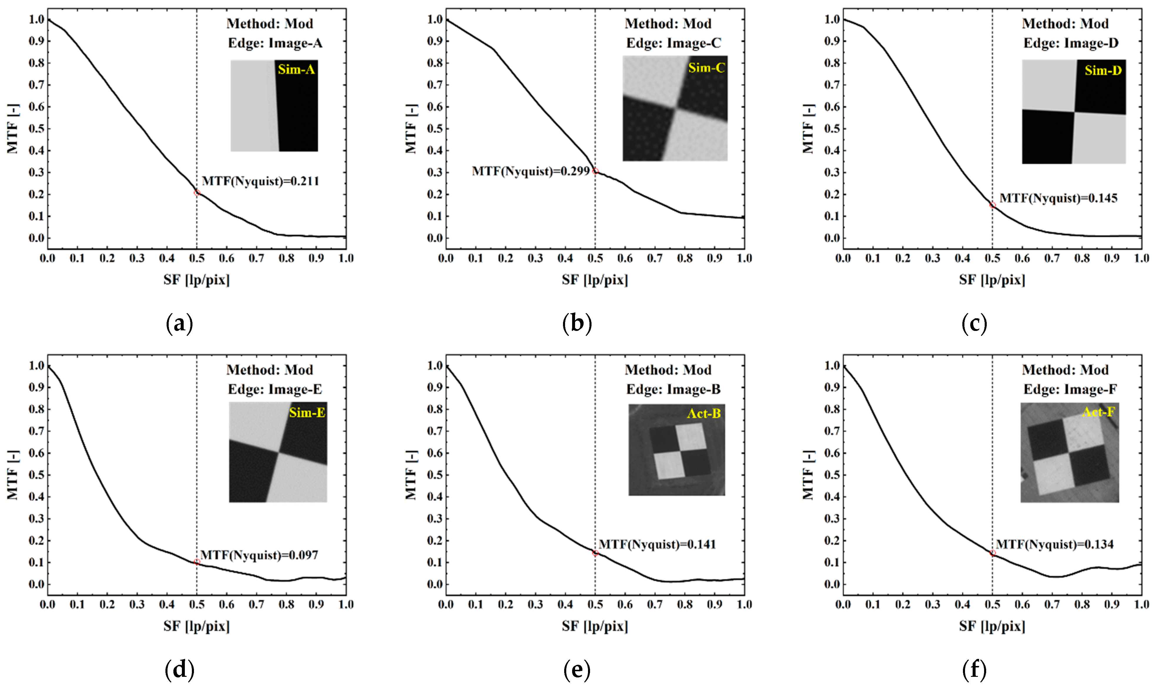
	MTF	Mod MTF at Nyquist Frequency	Reference [1] MTF Average at Nyquist Frequency
Edge Image
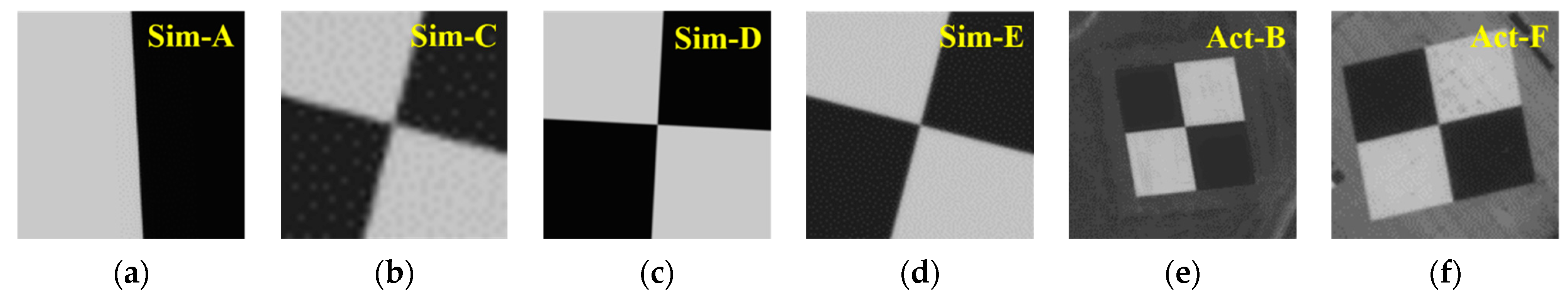
Simulated edge image A		0.221	0.20~0.21
Simulated edge image C		0.299	0.29~0.30
Simulated edge image D		0.145	0.12~0.14
Simulated edge image E		0.097	0.08~0.10
Actual edge image B		0.141	0.13~0.14
Actual edge image F		0.134	0.12~0.13

.

From the comparison of MTF measurement results in Table 3, it can be seen that the MTF of edge images A, D, B, and F measured by the Mod edge method is slightly higher than the measurement reference value provided in reference [1], but the measurement error is kept within 0.01, which verifies the effectiveness of the Mod edge method. On the one hand, it is related to the insufficient adaptability of the existing MTF compensation model. On the other hand, it is related to the generally low MTF measurement result of the existing edge method, which mostly adopts a single large ROI.

5.3. Discussion of Influencing Factors

Quantitative suggestions on the influencing factors and the performance of the Mod edge method are summarized as follows:

(1) It is reasonable to measure multidirectional MTF by using edges with different angles. For [0, 45] deg edge images, the MTF curves decrease with the increase of edge angle, but the consistency of MTF curves obtained by [0.2, 14.5] deg edge in the whole frequency ranges is obviously higher than that of other angle intervals.

(2) The MTF measurement accuracy is higher when the ideal optimal or suboptimal OSR calculated based on 1/[k·tan(θ)] (k∈Z₊) is adopted, and the minimum computational cost is realized. However, when the calculated OSR is too high (>10) or too low (<2), the actual OSR can be corrected to 8 or 2 to balance the computational cost and MTF measurement accuracy.

(3) The extracted ROI-H should be increased as much as possible to contain more edge information which can improve the MTF accuracy in middle and high frequency ranges. In practice, the ROI-H ratio of extracted ROI should be above 0.5 at least. On this basis, the ROI-W can be appropriately increased to ensure MTF stability in low frequency ranges.

(4) It is necessary to add contrast verification to ensure the determined edge contrast is greater than 0.1, thus ensuring the accuracy and effectiveness of the edge method. Although contrast has little impact on the edge method, it is recommended to give priority to high-contrast edge images when other conditions are consistent.

(5) It is necessary to add SNR verification to ensure the determined edge SNR is greater than 10 dB, thus ensuring the effectiveness of the edge method. When the SNR is lower than 10 dB, appropriate denoising should be done first. It is suggested that only the gentle regions on both sides of the edge should be denoised to keep the original features near the edge most.

6. Conclusions

In this paper, the effects of edge angle, OSR, ROI, edge contrast, and random noise on the accuracy of the edge method are quantitatively analyzed, which can provide a universal parameter determination reference for MTF measurement in different imaging fields. According to the results of quantitative analysis, a modified practical multidirectional edge method for MTF measurement is proposed. The adaptive determination model of optimal OSR and binning PS based on edge angle is established, and the automatic extraction model of multi-region and multi-size ROI based on edge angle and the image size is established. On the premise of ensuring the effectiveness of the edge method, the Mod edge method solves the problem of weak robustness caused by actual complicated edge image quality through a more reasonable OSR model and statistical method. Moreover, the Mod edge method has certain anti-noise ability and engineering practicability and is more robust in multidirectional MTF measurement.

References

- Viallefont-Robinet, F.; Helder, D.; Fraisse, R.; Newbury, A.; van den Bergh, F.; Lee, D.; Saunier, S. Comparison of MTF measurements using edge method: Towards reference data set. Opt. Express 2018, 26, 33625–33648. [Google Scholar] [CrossRef] [PubMed]
- Masaoka, K.; Yamashita, T.; Nishida, Y.; Sugawara, M. Modified slanted-edge method and multidirectional modulation transfer function estimation. Opt. Express 2014, 22, 6040–6046. [Google Scholar] [CrossRef] [PubMed]
- Viallefont-Robinet, F.; Leger, D. Improvement of the edge method for on-orbit MTF measurement. Opt. Express 2010, 18, 3531–3545. [Google Scholar] [CrossRef] [PubMed]
- ISO 12233:2017; Photography-Electronic Still Picture Imaging-Resolution and Spatial Frequency Responses, document ISO 12233:2017. Multiple. Distributed through American National Standards Institute (ANSI) : Washington, DC, USA.
- Duan, Y.X.; Xu, S.B.; Yuan, S.C.; Chen, Y.Q.; Li, H.G.; Da, Z.S.; Gao, L.M. Modified slanted-edge method for camera modulation transfer function measurement using nonuniform fast Fourier transform technique. Opt. Eng. 2018, 57, 014103. [Google Scholar] [CrossRef]
- Zhang, H.S.; Li, C.; Duan, Y.X. Modified slanted-edge method to measure the modulation transfer function of camera. Optik 2018, 157, 635–643. [Google Scholar] [CrossRef]
- Masaoka, K. Edge-based modulation transfer function measurement method using a variable oversampling ratio. Opt. Express 2021, 29, 37628–37638. [Google Scholar] [CrossRef] [PubMed]
- Li, T.C.; Feng, H.J.; Xu, Z.H. A new analytical edge spread function fitting model for modulation transfer function measurement. Chin. Opt. Lett. 2011, 9, 031101. [Google Scholar] [CrossRef]
- Xie, X.F.; Fan, H.D.; Wang, A.D.; Zou, N.Y.; Zhang, Y.C. Regularized slanted-edge method for measuring the modulation transfer function of imaging systems. Appl. Opt. 2018, 57, 6552–6558. [Google Scholar] [CrossRef] [PubMed]
- Li, X.B.; Jiang, X.G.; Zhou, C.J.; Gao, C.X.; Xi, X.H. An analysis of the knife-edge method for on-orbit MTF estimation of optical sensors. Int. J. Remote Sens. 2010, 31, 4995–5010. [Google Scholar] [CrossRef]
- Masaoka, K. Accuracy and Precision of Edge-Based Modulation Transfer Function Measurement for Sampled Imaging Systems. IEEE Access 2018, 6, 41079–41086. [Google Scholar] [CrossRef]
- Xie, X.F.; Fan, H.D.; Wang, H.Y.; Wang, Z.B.; Zou, N.Y. Error of the slanted edge method for measuring the modulation transfer function of imaging systems. Appl. Opt. 2018, 57, B83–B91. [Google Scholar] [CrossRef] [PubMed]
- Maruyama, S. Assessment of uncertainty depending on various conditions in modulation transfer function calculation using the edge method. J. Med. Phys. 2021, 46, 221–227. [Google Scholar] [PubMed]
- Masaoka, K. Real-time modulation transfer function measurement system. In Proceedings of the Proc. SPIE Conference on Ultra-High-Definition Imaging Systems II, San Francisco, CA, USA, 2–3 February 2019; Volume 10943, p. 1094309. [Google Scholar]
- Masaoka, K. Practical edge-based modulation transfer function measurement. Opt. Express 2019, 27, 1345–1352. [Google Scholar] [CrossRef] [PubMed]
- Masaoka, K. Line-Based Modulation Transfer Function Measurement of Pixelated Displays. IEEE Access 2020, 8, 196351–196362. [Google Scholar] [CrossRef]
- Zengilowski, G.R.; McMurtry, C.W.; Pipher, J.L.; Reilly, N.S.; Dorn, M.L.; Mainzer, A.K.; Wong, A.F.; Reinhart, L.; Newswander, T.; Luder, R. Modulation transfer function measurements of HgCdTe long wavelength infrared arrays for the Near-Earth Object Surveyor. J. Astron. Telesc. Instrum. Syst. 2022, 8, 23. [Google Scholar] [CrossRef]
- Wang, C.; Zhu, R.F. Optical satellite image MTF compensation for remote-sensing data production. Int. J. Comput. Appl. Technol. 2022, 68, 132–142. [Google Scholar] [CrossRef]
- Takeuchi, T.; Hayashi, N.; Asai, Y.; Kayaoka, Y.; Yoshida, K. Novel method for evaluating spatial resolution of magnetic resonance images. Phys. Eng. Sci. Med. 2022, 45, 487–496. [Google Scholar] [CrossRef] [PubMed]
- Kakinuma, R.; Kawagishi, N.; Yasugi, M.; Yamamoto, H. Influence of incident angle, anisotropy, and floating distance on aerial imaging resolution. OSA Continuum. 2021, 4, 865–878. [Google Scholar] [CrossRef]
- Fang, Y.-C.; Tsay, H.-L. A study of multi-angles knife-edge method applied to digital modulation transfer function measurement. Microsyst. Technol. 2021, 27, 1429–1437. [Google Scholar] [CrossRef]
- Roland, J.K.M. A study of slanted-edge MTF stability and repeatability. In Proceedings of the Proc. SPIE Conference on Image Quality and System Performance XII, San Francisco, CA, USA, 10–12 February 2015; Volume 9396, p. 93960L. [Google Scholar]
- Fang, Y.C.; Tzeng, Y.F.; Wu, K.Y.; Tsay, H.L.; Lin, P.M. Measurement and analysis of modulation transfer function of digital image sensors. Microsyst. Technol. 2022, 28, 137–142. [Google Scholar] [CrossRef]