1. Introduction
In order to realize high-speed and low-power operations, embedded neural network accelerators generally only support low-precision numerical operations, such as 8-bit or 4-bit low-bit integer operations. In contrast, the original numerical precision of neural network models is generally 32-bit floating-point numbers. Therefore, quantization algorithms need to be employed to compress the original network by reducing the number of bits of precision required to represent weights or activations [
1]. In the calculation process of the neural network accelerator deployed with the quantization algorithm, the number of data transfers can be effectively reduced, the bottleneck of transmission bandwidth can be reduced, and the calculation speed can be improved [
2]. Quantization converts the floating-point value of the neural network into a fixed-point integer value with a set of scale factors. These scale factors, sometimes also called quantization parameters, are calculated according to the dynamic range threshold and quantization bit width of the floating-point data during the conversion process. When the upper and lower boundaries of the data dynamic range threshold are symmetrical, it is called a symmetric quantization, and when they are asymmetrical, it is called asymmetric quantization. The goal of a quantization algorithm is to determine the quantization parameters of a neural network model.
This paper is an extended version of a conference paper [
3]. Unlike the conference paper, the method proposed here determines a quantization parameter generation method for the LSTM layer for processing sequential features. Multi-bit quantization retraining is added to be supported on CPU/GPU. This method is universal, the corresponding classical benchmark datasets are selected for evaluating different applications such as character-level language prediction, word-level language prediction, and image classification.
Many of the most widely used AI applications are now based on Long Short-Term Memory (LSTM) recurrent neural networks (RNNs), which learn from experience to solve all kinds of previously unsolvable problems. The LSTM principle has become a foundation of what is now called deep learning, especially for sequential data. LSTM-based systems can learn to translate languages; control robots; analyze images; summarize documents; recognize speech, videos, and handwriting; run chatbots; predict diseases, click rates, and stock markets; compose music; and much more [
4].
LSTM is mainly used to perform tasks in sequential data processing. It can effectively solve the problem of gradient explosion in RNN and can effectively capture the dependencies between contexts. In these real-time machine learning applications with sequential features, LSTM is severely limited by latency, energy, and size. In order to improve hardware efficiency, many researchers have proposed the use of the quantization technology of intelligent algorithms to relieve the technical pressure of platform computing power and improve computing efficiency.
However, there are two technical bottlenecks regarding LSTM quantization: one is the embedded computing platform, and the other is the quantization algorithm itself. We will start with a general overview from these two perspectives.
Technical Bottleneck 1: Most of the current embedded computing platforms do not directly support performing the quantization operation for the LSTM layer. There are two difficulties: (1) such hardware interfaces rely too much on neural network models; (2) there is a lack of quantization tools to support LSTM calculation.
Technical Bottleneck 2: The influence of sequential input properties of LSTM has not been taken into account by quantization algorithms. There are two problems: (1) ordinary quantization calibration images, which are used for regular layers, do not have sequential characteristics; (2) quantization calibration images adapted to LSTM do not ensure the diversity of quantization.
Aiming at these two technical bottlenecks in both the embedded computing platform and the quantization algorithm, this paper proposes a sequential-characteristics-based operators-disassembly-quantization method for LSTM layers. There are two innovations in this proposed method to improve the technical bottlenecks described above:
- (1)
We design an operators disassembly quantization process for the LSTM layer, so that the neural network accelerator can support the LSTM layer on the embedded platform.
- (2)
The quantization parameter generation process is designed as a sequential-characteristics-based combination strategy for LSTM quantization calibration. The advantages of this design are that sequential characteristics are added to the quantization algorithms. It breaks through the limitations of existing quantization methods that rely on the quantization calibration sets to be still images and can only support model structure with traditional layer types.
2. Related Works
The main acceleration targets of the current neural network accelerators on the embedded Field Programming Gate Arrays (FPGA) platform [
5] are typical neural network operators, such as convolution, full connection, pooling, etc. However, with the increasing complexity of the problems solved by deep learning technology, some new types of complex operators have gradually emerged, which are mainly represented by variant form models of RNN [
6], such as LSTM [
7] and GRU [
8]. The RNN neural network model is widely used in the field of natural language processing, but it has problems with vanishing or exploding gradients when processing large amounts of text.
The improved form of RNN is LSTM, which introduces three gated structures, the forget gate, the input gate, and the output gate, in the unit, which can effectively solve this problem. The forget gate is responsible for the selective deletion of the input information and the hidden state information output by the previous unit, the input gate is responsible for selectively storing the retained new information into the unit state, and the output gate is responsible for selectively outputting the information in the unit state to the hidden layer.
LSTM removes or adds information to the cell state, called gates: input gate (
), forget gate (
), output gate (
), cell input vector (
), cell state vector (
), and hidden state vector (
) can be defined as follows:
where
,
,
,
is the weight matrix of the input node;
,
,
,
is the weight matrix of the hidden state; and
,
,
,
is the bias term.
LSTM has been widely used in various sequential data predictions [
9]. In the field of text processing, LSTM can perform text classification, text sequence annotation, text translation, image generation text, text-generated speech, speech recognition [
10], etc. In the field of computer vision, LSTM is primarily used for video classification, image annotation, video annotation [
11], and recently popular visual Q&A. In the field of engineering practice, computation offloading in mobile edge computing can also be predicted by LSTM [
12].
The quantization for LSTM compresses the original LSTM network by reducing the numerical bit width of the model and reducing the calculation and inference time, and it has a direct relationship with the hardware. The specific quantization process for most quantization algorithms is as follows. It uses the layers as the basic processing unit. First, the distribution and range of weight and output data of each layer of the neural network model are analyzed in advance. Then, each floating-point value is represented by a low-bit integer based on the uniform-symmetric [
13] quantization strategy. Finally, the quantization-calibrated weights and activation thresholds, namely quantization parameters, are calculated to generate a guide file for the neural network accelerator to map floating-point data into integer data.
The quantization strategy of mapping floating-point data to integer data is to select a reasonable threshold based on the dynamic range of the data to ensure that the loss of information is minimized. Therefore, the original information is truncated before mapping through the threshold, and it is mapped to a low bit-precision range. This avoids the problem of wasted dynamic range resources. There are many quantization strategies for selecting thresholds, such as the minimum–maximum (MIN–MAX) quantization strategy used by Tengine, which makes the absolute maximum value the threshold value. Taking 8-bit quantization as an example, we can see that it is proportionally mapped to the range of plus or minus 127. This simple MIN–MAX clipping only works for uniform distributions. When the data are non-uniformly distributed, the loss of dynamic range can cause a considerable loss of accuracy. Most users, such as NVIDIA, have proposed using the KL-divergence (KLD)-based method [
14] to measure the degree of difference in the distributions before and after the quantization to find the optimal threshold value. KL divergence has some disadvantages, such as being unbounded asymmetric, and the results obtained are meaningless if the two distributions do not overlap. There are also some other quantization strategies that use the average–maximum (AVG–MAX), Easy Quant [
15], etc., to determine the optimal threshold value. AVG–MAX takes the average value according to the change in value, taking into account the principles of simplicity and balance. EasyQuant achieves close to Int8 and Float32 performance even at Int7 or lower bits. However, its accuracy and performance advantages over KLD are mainly reflected in the int7 type, and the accuracy of int8 seems similar to KLD. Google’s TensorFlow [
16] applies exponential moving averages (EMA) for the activation quantization, which calculates the bounds of activations on the fly. It modifies the bounds after each iteration, which is too frequent to be suitable for quantization parameter learning. The comparison table of key characteristics and limitations of different quantization strategies is shown in
Table 1.
We want to achieve LSTM quantization that performs as well as quantization on the regular layers. For this purpose, we analyze previous quantization methods and observe that, at present, the quantization of the LSTM layer still has the following two problems:
- (1)
LSTM has not only high-density computation such as matrix-vector multiplication [
17] but also has complex control flow, which will significantly affect the execution speed of LSTM [
18]. It is implemented on a specific FPGA platform [
19]. However, such hardware interfaces rely too much on neural network models and hardware platforms and lack generality [
20].
- (2)
Most of the current general-purpose neural network accelerators cannot directly support the quantization calculation of LSTM. Firstly, the LSTM layer cannot be directly executed by the neural network accelerator on the embedded FPGA platform. Secondly, there is a lack of quantization tools to support LSTM calculation [
21]. Even if the LSTM layer is converted into an existing regular layer, the traditional quantization calibration methods are still applied; i.e., sequential characteristics are not taken into account. That is, all quantization calibration sets are repeatedly fed into each time step of the LSTM as input. The activation quantization threshold is selected according to the distribution of layer-by-layer output data, regardless of the size of the time step [
22]. It is very easy to cause the quantization dataset of the LSTM layer not to have diversity and sequential consistency, which in turn leads to a considerable loss of quantization accuracy.
Therefore, aiming at the neural network model fused with LSTM layers based on sequential data, it is necessary to design a quantization method for neural network models that integrates the LSTM layer.
That is, on the one hand, the LSTM layer is split from the software level into multiple basic operators supported by the neural network accelerator, so that the neural network accelerator can support the LSTM layer on the embedded platform, and it can be combined with the traditional model quantization algorithm to broaden the scope of application of the quantization algorithm.
On the other hand, the combination strategy using quantization calibration sets takes into account the sequential characteristics of the LSTM layer. The combined images are designed for the quantization calibration of regular layers. When encountering the LSTM layer, according to the time step of LSTM, the diverse image groups are gradually sent to each time step, where each diverse image group has sequential characteristics. It solves the hardware deployment problem of the sequential forecasting model and improves the accuracy of the quantization algorithm. This not only ensures the diversity and scientificity of quantization but also improves the quantization accuracy of models with LSTM layers.
3. Proposed Methodology
3.1. Problem Definition
The quantization method for LSTM layers deployed on neural network accelerators discussed in this paper is as follows.
- (1)
The embedded computing platforms such as the neural network accelerator deploying the neural network models need to quantize the values into low-bit integers through quantization operations. However, most of the current embedded computing platforms with a fixed-point architecture do not directly support performing the quantization operation for the LSTM layer. The original structure of LSTM consists of 6 types of mapping as shown in Equations (1)–(6), named
, respectively. However, embedded computing platform (such as NPU) can only handle mapping cases with linear or nonlinear relationships such as
,
or
. Therefore, we divide the LSTM layer into a set of regular layers, and its computation process is a combination of the fully connected layer (FC), the Eltwise layer (Eltwise Add, Eltwise Prod), and the nonlinear layer (Sigmoid, Tanh). That is, as shown in Equation (7), we strive to find a correspondence
between the LSTM and the NPU in this paper, and split and map the LSTM into a certain type of Y supported by NPU.
- (2)
LSTM is mainly used to perform tasks in sequential data processing. However, the influence of sequential input data of LSTM has not been taken into account by quantization algorithms. Aiming at this bottleneck, the goal of the proposed quantization algorithm is to determine the quantization parameters of neural network models with the LSTM layer and deploy them on the NPU. The original numerical precision of neural network models is generally 32-bit floating-point numbers. The core computation of a 32-bit floating-point model can be expressed as
. Since NPU only supports integer matrix multiplication, quantization converts the floating-point weight
and activation
of the neural network into a fixed-point integer value
and
by
, as shown in (8), where
and
are called quantization parameters.
Therefore, the calculation of can be performed on the NPU. However, it will cause . Therefore, needs to be inversely quantized to by . Then, finding the reasonable values of the quantization parameters and becomes the problem that needs to be solved in this paper.
3.2. Overall Method Design
The proposed quantization method combines the quantization operation with the neural network accelerator hardware. It is described in detail below. First of all, the operators’ disassembly is designed so that the calculation process of LSTM is split into layer-by-layer calculation sequences. Then, the quantization calibration process is designed as a sequential-characteristics-based combination strategy for sequential and diverse image groups. The input and output vectors of the separated LSTM are reasonably connected to the existing traditional type layer. Finally, the quantization parameters are generated and deployed on the embedded computing platform (such as NPU) for accuracy calculation testing.
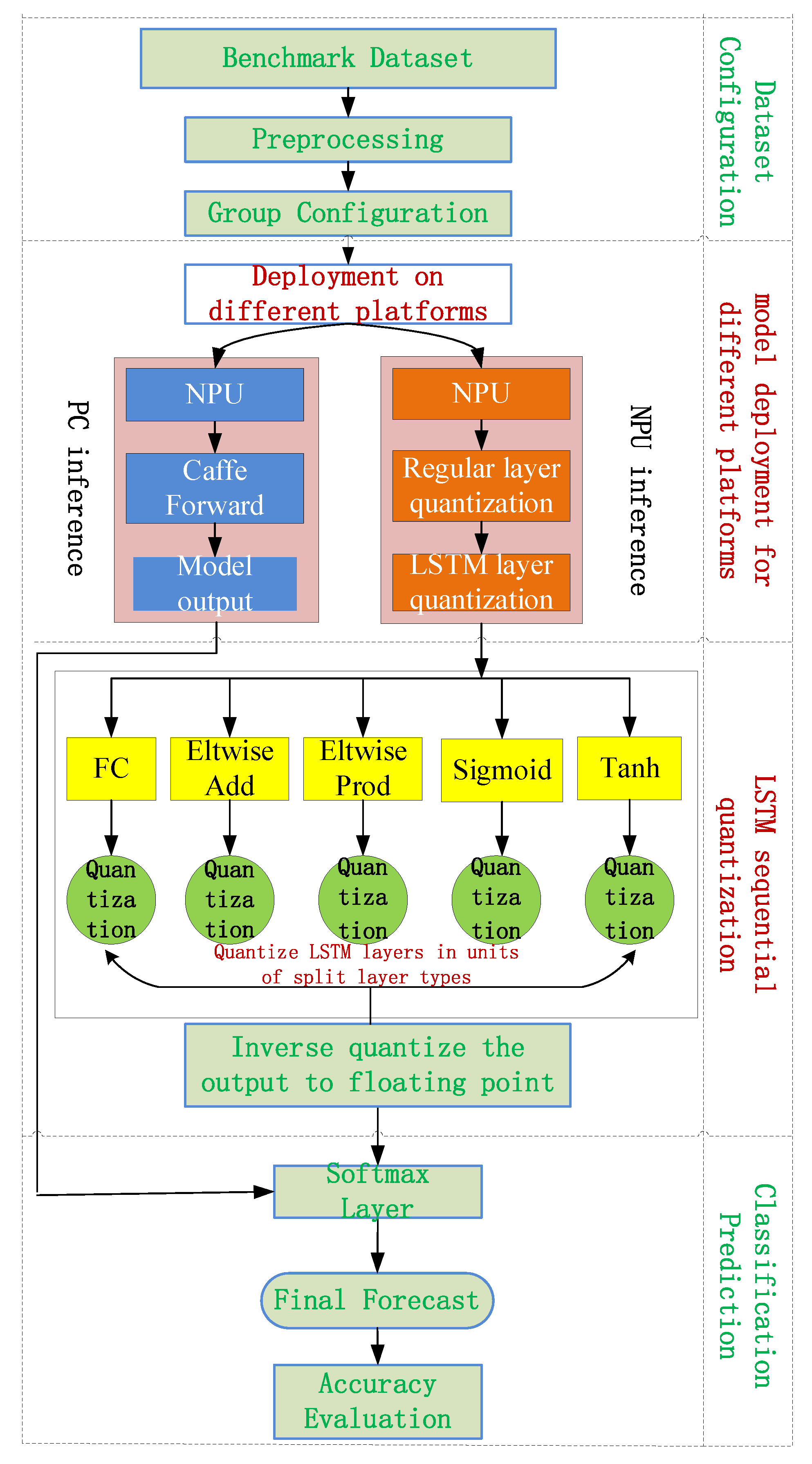
In this section, we begin specific hardware and software deployment design processes. In order to design a quantization deployment scheme for LSTM layers and verify the effectiveness of the scheme, it is necessary to deploy models on different platforms for specific data sets, including PC and NPU. Quantization is carried out for the hardware platform. Finally, the model inference outputs on different platforms are classified and predicted, and the accuracy evaluation is given. The overall design process is shown in
Figure 1.
The overall method design consists of four parts; dataset configuration, model deployment for different platforms, LSTM sequential quantization, and classification prediction. The specific breakdown is as follows:
Part I: Firstly, configure a reasonable dataset set for different platforms. Secondly, set up a certain number of quantization calibration sets for the hardware platform. Thirdly, design the quantization calibration process as a sequential-characteristics-based combination strategy for sequential and diverse image groups. See
Section 3.4 for details.
Part II: On the PC side, the model is pushed forward based on the Caffe deep learning software framework. On the NPU side, the quantization deployment of the hardware platform is carried out. For a neural network model with both regular and LSTM layers, the existing uniform-symmetric quantization is performed on the regular and LSTM layers.
Part III: The detailed process of LSTM layer quantization on the hardware platform is as follows: the LSTM layer is divided into a set of regular layers, and its computation process is a combination of the fully connected layer (FC), the Eltwise layer (Eltwise Add, Eltwise Prod), and the nonlinear layer (Sigmoid, Tanh). It is reasonably connected with other regular layers of the model to generate quantization parameters and deploy them on the neural network accelerator. See
Section 3.3 for details.
Part IV: Finally, the quantized output of the NPU side is inverse-quantized to a floating-point representation type. The model outputs on the PC and NPU side are separately classified and predicted, and the accuracy evaluation results are given.
The proposed method determines a quantization-parameter-generation method for the LSTM layer for processing sequential features. Multi-bit quantization retraining is supported on CPU/GPU. This method is implemented entirely on a hardware with a fixed-point architecture. Once complex quantization training is completed offline, the quantized LSTM model can be directly deployed on the embedded neural network accelerator. It not only quickly implements the support of the embedded computing platform for the LSTM but also effectively improves the quantization accuracy of the model.
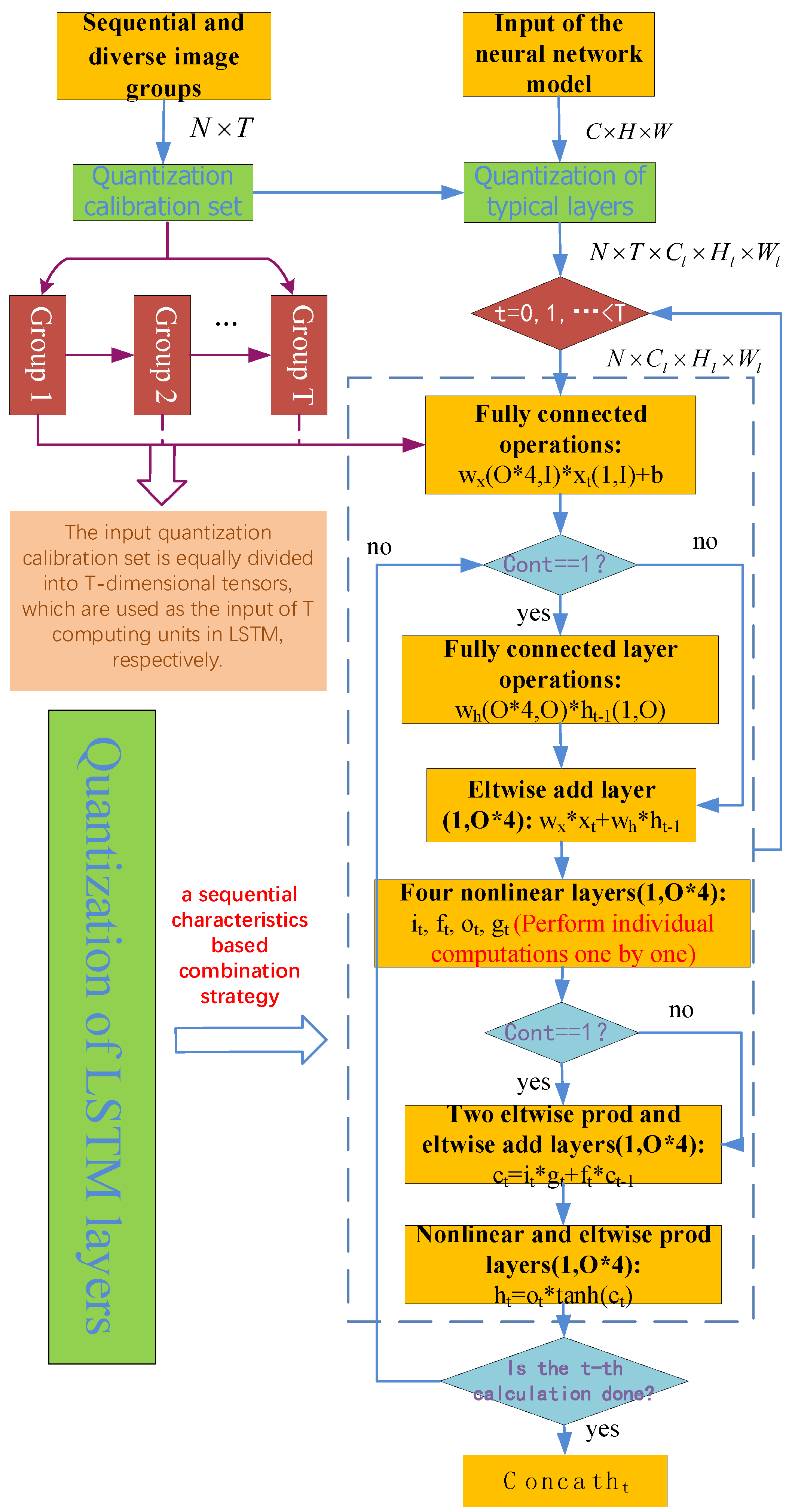
3.3. LSTM Operators Disassembly Design
The LSTM is a specific network layer in the neural network model, but the computational logic of this layer is more complex than the typical layer. The input of the LSTM layer is and , and the output is . is a tensor of (T, I), where T is the time step and I is the input feature dimension. is a continuity identifier, consisting of 0, 1, where 0 means start and 1 means continuous, and the dimension is T. is a tensor of (T, O), where O is the output feature dimension.
LSTM first divides the calculation into T small computing units and then divides into T (1, I) tensors equally according to the size of the time step T, named , respectively. These T divided inputs will be used as the input of each computational unit in the LSTM. It is worth noting here that and are all-zero tensor sequences (1,O), and and are the result of the previous and . Finally, the sequence of T tensors (1, O) from to are combined into one output (T, O) as the output of the LSTM layer.
In the specific Caffe implementation process, the input of LSTM can be expressed as , so we use two fully connected layers to replace the matrix multiplication operations in Equations (1)–(4). The first is , and the second is , where , , .
In terms of layer type, Equations (1)–(6) are divided into the LSTM layer operation processes calculated in the following 9-layer order:
Layer 3—Eltwise Add layer:
Layer 4—Non-linear layer:
Layer 5—Eltwise Prod layer:
Layer 6—Eltwise Prod layer:
Layer 7—Eltwise Add layer:
Layer 8—Non-linear layer:
Layer 9—Eltwise Prod layer:
Because hardware accelerators can only process integer data, when we perform nonlinear function operations, there are two steps in total. The first step is to build a nonlinear lookup table in the quantization software. If there are two nonlinear functions, two lookup tables are created. The specific operation is to first dequantize all integer values in the bit width range to a floating point according to the inverse of Equation (8). The dequantized floating-point values are then mapped according to the nonlinear functions sigmoid and tanh, respectively. Finally, the mapped value is quantized to an integer again according to Equation (8). The sequence of input integers and output integers form a lookup table. The second step is to feed the lookup table into the neural network accelerator. The corresponding rules between the source register and the destination register are used to map one-by-one to complete the calculation of the nonlinear layer.
3.4. LSTM Sequential Quantization Design
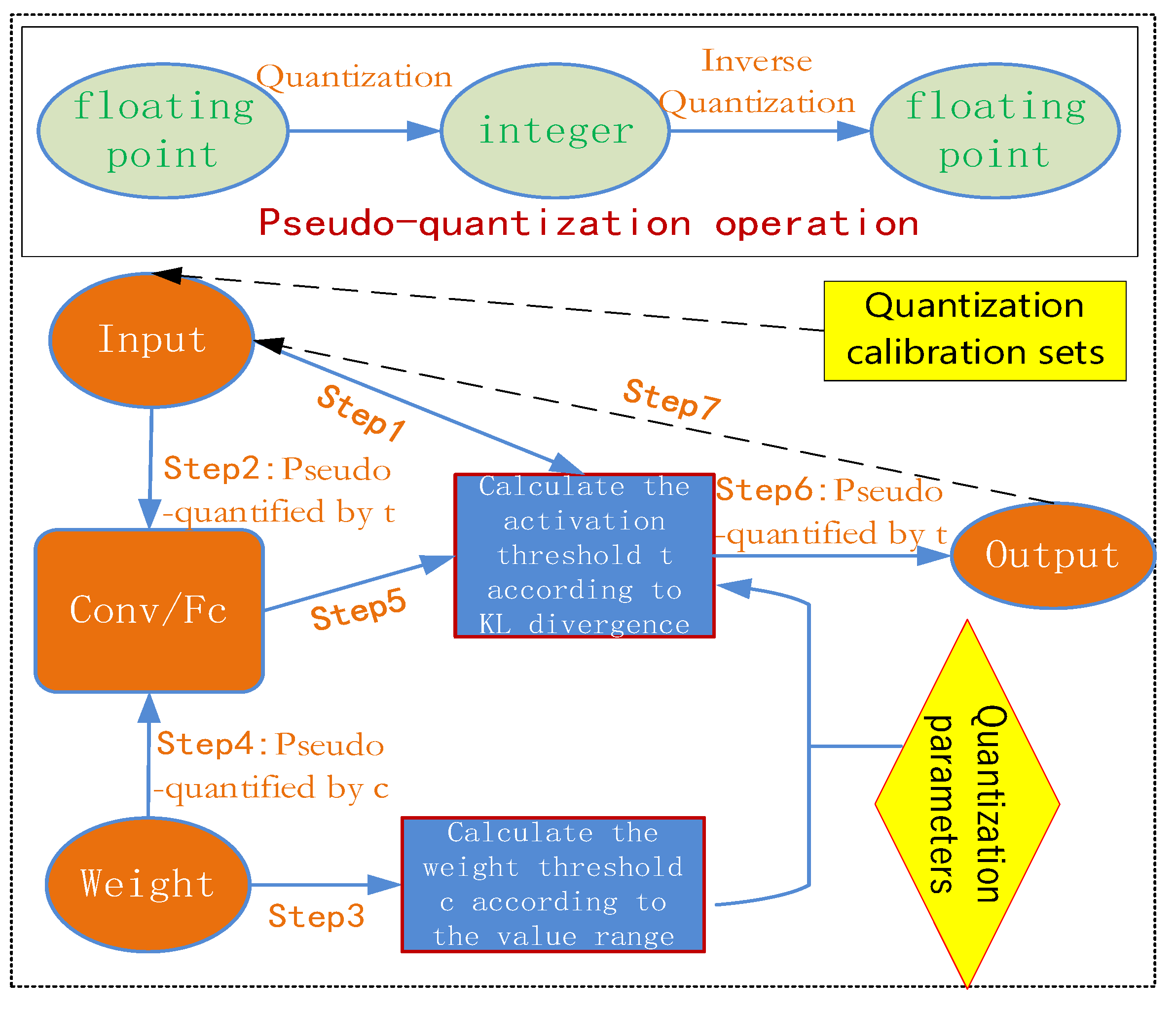
The LSTM layer is disassembled and becomes a collection of many regular layers, and the quantization calibration method of the regular layers can also be applied. That is, all quantization calibration sets are first fed into the regular layers in front of the LSTM, and the activation quantization threshold is selected according to the distribution of layer-by-layer output data. When encountering an LSTM layer, regardless of the size of the time step, the input quantization calibration set is repeatedly fed into each time step of the LSTM as input to each computational unit in the LSTM. Finally, each output tensor sequence is combined into a single output as the output of the LSTM layer. However, since the LSTM layer processes datasets that have sequential characteristics, once processed according to the basic methods as shown in
Figure 2, it is very easy to cause a large loss of quantization accuracy.
Our basic quantization algorithm is described in detail as follows. When the quantization algorithm generates quantization parameters of regular layers and LSTM layers, a pseudo-quantization operation is inserted into the weight and output of each layer. That is, the floating-point value is first quantized to a low-bit integer and then inversely quantized back to a floating-point value. Each time, the pseudo-quantized values are used to perform operator calculations, such as convolution, pooling, upsampling, etc. After the calculation is completed, pseudo-quantization is performed again, and the quantization parameters are counted and sent to the next layer. The output of the current layer is used as the input of the next layer and so on. Note that the first layer requires additional pseudo-quantization operations on the input. The overall flow chart of the quantization algorithm for neural network models that integrates the LSTM layer is shown in
Figure 2.
In this section, the quantization calibration process is designed as a sequential-characteristics-based combination strategy for LSTM quantization calibration. The neural network model integrating LSTM layers has both regular layers and LSTM layers. The quantization calibration set of the network model built only for regular layers is relatively simple. Many diverse image groups with different categories, backgrounds, angles, and lightings are selected. The data processed by LSTM are generally sequential; that is, the data collected at different times for the described phenomenon over time. Therefore, this paper designs the sequential-characteristics-based combination strategy of sequential and diverse image groups.
Assuming that the time step of the LSTM layer is
T, the model input size is
C ×
H ×
W. Thus,
diverse image datasets groups of different categories, different backgrounds, different angles, and different lightings are selected. Each group contains
T groups of sequential datasets with training consistency; that is, the dimension of the quantized calibration set is
. On the one hand, the combined
images are used for the quantization calibration of regular layers. On the other hand, when encountering the LSTM layer, according to the time step of LSTM,
diverse image groups are gradually sent to each time step, where each diverse image group has sequential characteristics. The specific quantization calibration process is shown in
Figure 3.
More precisely, when generating the quantization parameters, firstly all the groups data are sent to the regular layer, the activation quantization threshold is selected according to the output data distribution of this layer, and the data dimension of each layer l is N × T × Cl × Hl × Wl. When the LSTM layer is encountered, according to the size of the time step T, the input quantization calibration set is equally divided into T tensors of dimension, which are, respectively, used as the input of the T computing units in the LSTM. Weights and activation quantization thresholds are selected layer by layer according to the weights and activation output distribution ranges for sets of input data. Finally, the T output tensor sequences are combined into one output as the output of the LSTM layer. At this time, if there is still a regular layer after the LSTM layer, we continue to calibrate the sets of output data to the subsequent layers.
4. Experiments
In this section, quantization experiments are carried out to verify the proposed quantization method’s effectiveness.
First, we describe the implementation details of the proposed quantization method in
Section 4.1. Then, most importantly, we compare the experimental results in the relevant literature with the methods proposed in this article from character-level language prediction, word-level language prediction, and image classification in
Section 4.2. Then, in
Section 4.3, we perform the ablation experiment of the algorithm itself from the perspectives of sequential quantization calibration and activation quantization clipping. In addition, considering the acceleration requirements of the actual hardware architecture implementation, performance analysis is conducted in
Section 4.4 for the quantization deployment of CPU, GPU, and NPU, respectively.
4.1. Implementation Details
This section first gives the experimental settings for the following three types of experiments. Then, the principles of quantization implementation and the basic software that the experiment relies on are described in detail.
4.1.1. Experiment Settings
The experimental settings and evaluation metrics are shown in
Table 2. In comparison experiments with the state of the art, character-level language prediction application is performed on two datasets: (i) Leo Tolstoy’s War and Peace and (ii) Penn Treebank Corpus [
23]. Performance Evaluation metrics are bits per character (BPC), variation in BPC, and size of LSTM parameters. In a word-level language-prediction application, Penn Treebank dataset was selected and evaluated by the perplexity per word (PPW), variation in PPW, and relative MSE. The UCF101 dataset is used in image classification applications. Both ablation experiments were performed on the UCF101 dataset and evaluated by the Acc Loss (Top1). Performance experiments are conducted by running speed for the quantization deployment platforms of CPU, GPU, and NPU, respectively.
4.1.2. Experimental Details
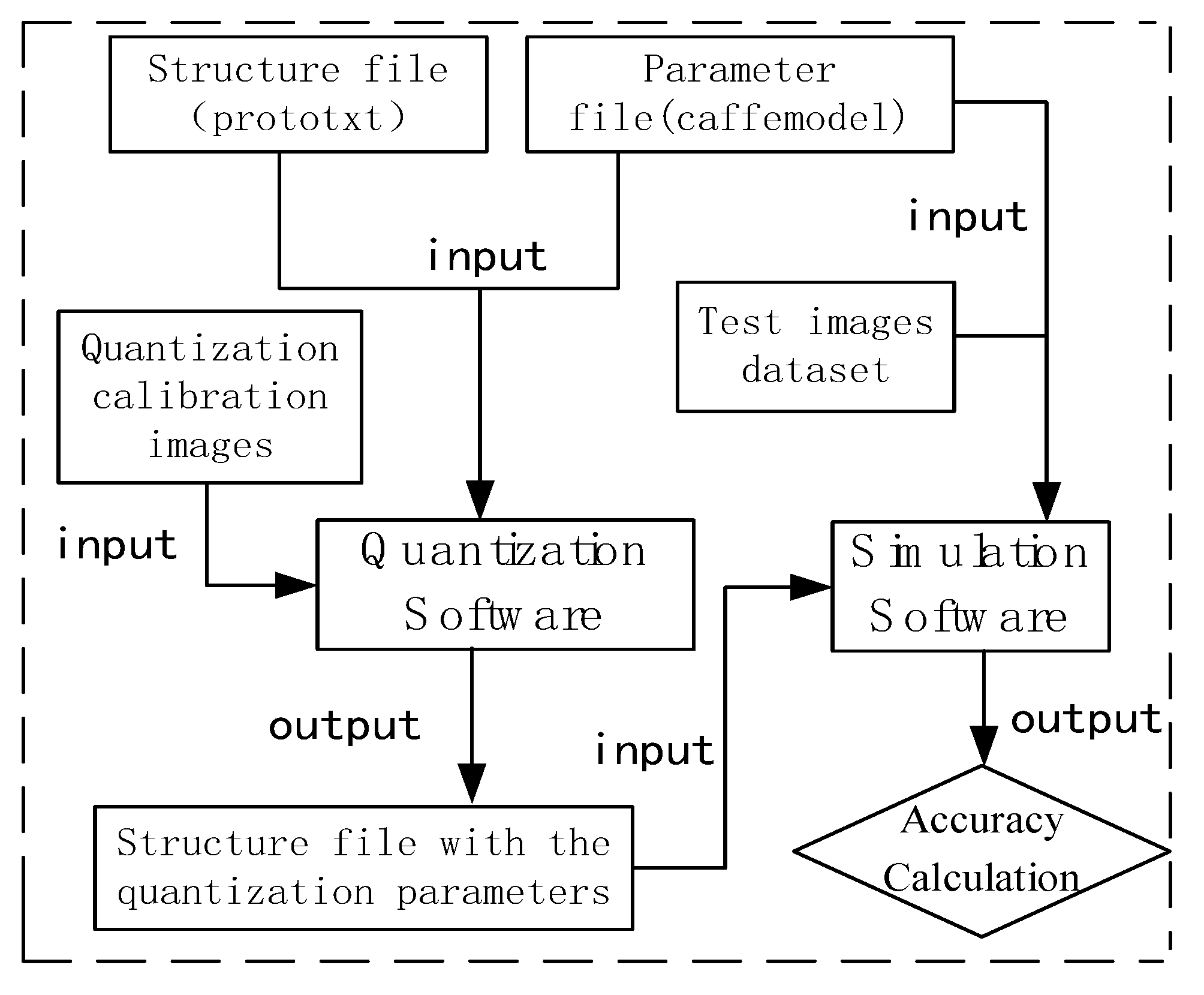
The methodology described in
Section 3 was implemented as two software tools based on the Caffe. These tools are quantization and simulation software, which are designed to complete the generation of quantization parameters and the NPU calculation simulation [
24]. The quantization software pre-analyzes the distribution and range of data at each layer of the network model, calculates the quantization parameters, and generates a guide file for the NPU to map floating-point data to low-precision data. Then, the simulation software simulates the runtime and NPU calculation process to verify the correctness of the hardware calculation results.
The inputs of the quantization software shown in
Figure 4 include the structure file (prototxt) and the parameter file (caffemodel) of the model, and the quantization calibration images. The output is the structure file with the quantization parameters added. The quantization parameters are used to guide the NPU to map floating-point data into integer data. Therefore, the structure file with the quantization parameters added, the parameter file, and the test image dataset make up the inputs to the simulation software. Its output is the accuracy calculation results.
In detail, this is accomplished by taking two steps for each layer: one for the weights and one for the activations. For the weight, count the weight threshold c of the current layer according to the value range, truncate the weight of the current layer to the [−c, c] interval, and then use the uniform-symmetric quantization method to quantize the weight, as shown in the following equation:
where the scaling factor
is obtained by the weight threshold
and the quantization bit width
:
For activation values, the quantization method is similar, except for one point, where the activation threshold
is chosen by finding the optimal value
that minimizes the KL divergence in the original activation value distribution and the quantized activation value distribution:
Therefore, the quantization algorithm is deployed on the embedded neural network accelerator according to the weights and activation thresholds generated above, namely quantization parameters. According to the quantization parameter threshold and bit width of the current layer, the quantization coefficient is calculated according to Equation (19). Then, the signed integer weight is calculated according to Equation (18) and the activation thresholds are generated according to Equation (20). Finally, the output of the last layer of NPU calculation is inverse-quantized into floating-point values.
4.2. Comparison with the State of the Art
In order to verify the effectiveness of the improved LSTM quantization method, comparison experiments with related works are carried out.
Experiments are performed on character-/word-level language modeling. We compare the full-precision LSTM and popular state-of-the-art quantized LSTMs, including (i) 1-bit LSTMs, binarized using BinaryConnect (BCN) [
25], binary weight network (BWN) [
26], and loss-aware binarization (LAB) [
27]; (ii) 2-bit LSTMs, ternarized using ternary weight networks (TWN) [
28] and loss-aware ternarization with approximate solutions (LAT) [
29]. Analogous to BinaryConnect, we also include a baseline called TerConnect1, which ternarizes weights to {−1, 0, +1} using the same threshold as TWN but does not scale the ternary weights. (iii) Multi-bit LSTMs: For simplicity of notation, we denote all the compared multi-bit quantization methods, including uniform [
30], balanced [
31], greedy [
32], refined greedy [
32], and alternating LSTM [
33] quantization as Uniform, Balanced, Greedy, Refined, and Alternating, respectively. Above all, we apply these methods to quantize the full precision pre-trained weight (activation is not quantified) of the single LSTM layer.
4.2.1. Character-Level Language Prediction
The LSTM takes as input a character sequence and predicts the next character at each time step. The training objective is the cross-entropy loss over target sequences, and performance is evaluated by bits per character (BPC). Experiments were performed on two benchmark datasets: (i) Leo Tolstoy’s War and Peace and (ii) Penn Treebank Corpus. On War and Peace and Penn Treebank, we used a one-layer LSTM with 512 hidden units as in [
34]. Adam is used as the optimizer.
Table 3 shows the testing BPC values and size of LSTM parameters. The method with the lowest BPC in each group is highlighted.
Comparison with Full-Precision LSTM: On both the Penn Treebank and the War and Peace datasets, the 2-bit, 4-bit, and 8-bit quantized LSTM performs similarly to the full-precision baseline. Moreover, compared with the full-precision LSTM, the 1-bit quantized LSTM has competitive performance but requires much less storage.
Comparison of Different Quantization Methods: For the quantized 1-bit LSTM, BWN and LAB perform significantly better than BCN. They have an additional scaling parameter, which is empirically smaller than 1, and can thus alleviate the exploding-gradient problem. Regardless of the dataset, compared to other comparison methods, our quantization method achieves the lowest BPC values by 1.446 and 1.723 in the 2-bit precision, respectively. The 4-bit and 8-bit quantized LSTMs also achieved relatively small quantization errors and have certain competitive performance advantages.
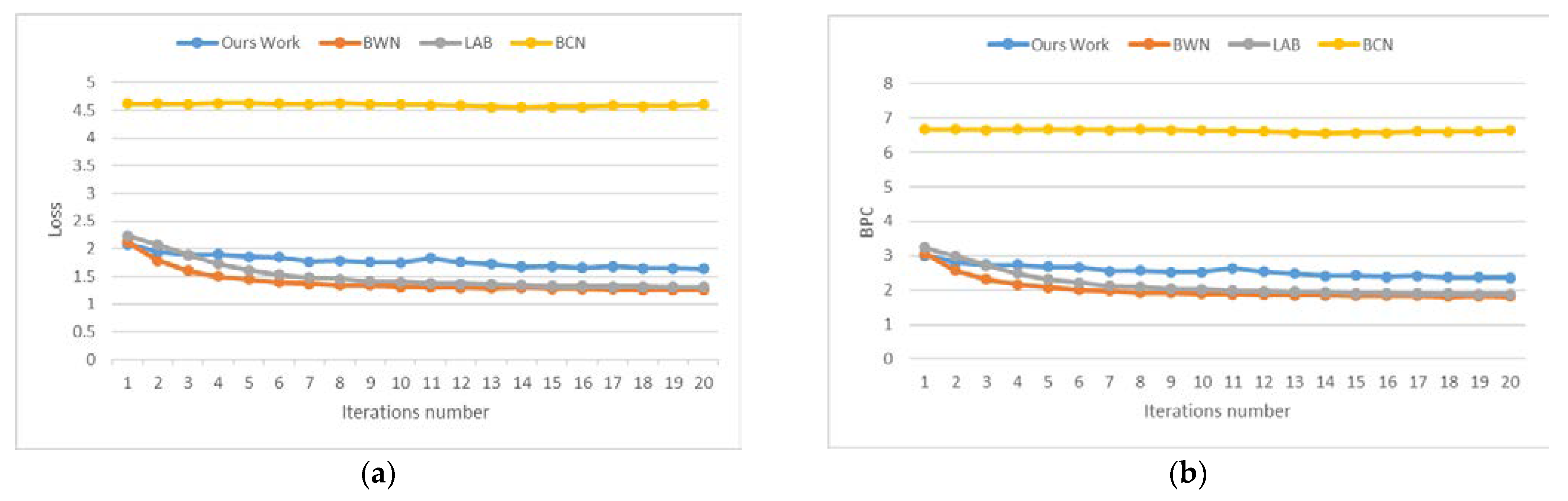
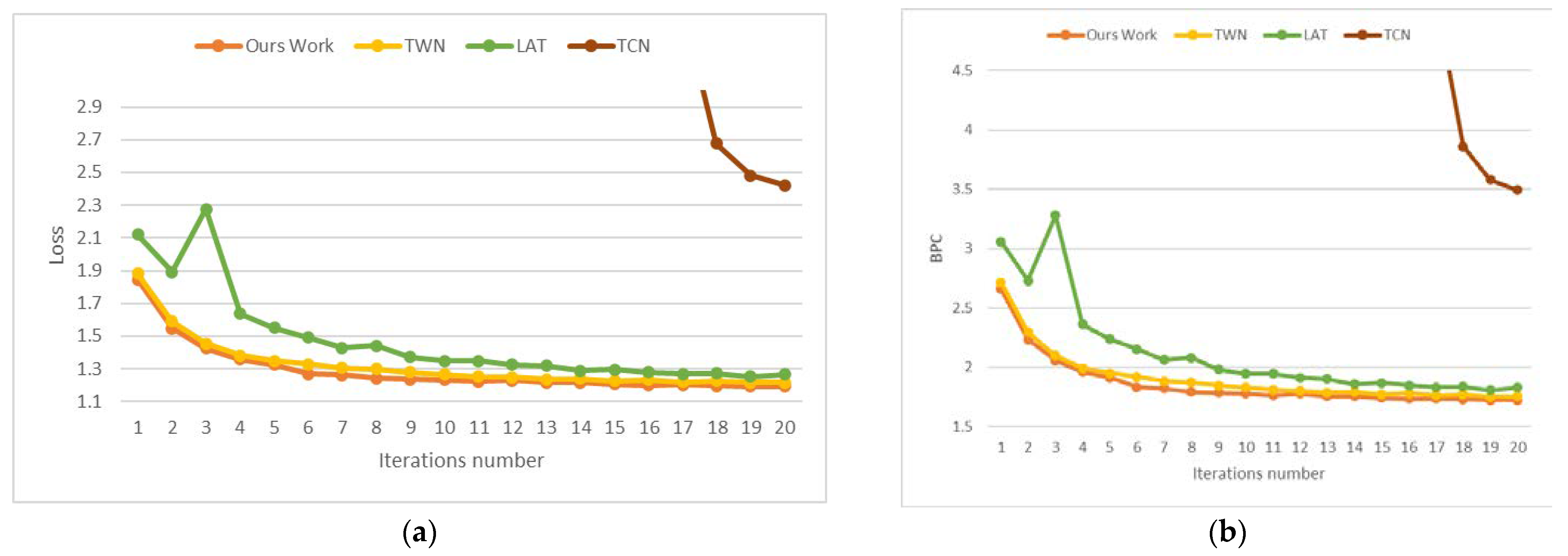
The loss function and BPC iteration curves for quantization retraining at different quantization precisions are shown in
Figure 5 and
Figure 6. As can be seen from
Figure 5, the loss and BPC of our method drops faster than the BCN in the 1-bit quantization precision, which is the same as other methods. As shown in
Figure 6, our loss and BPC values converge the fastest of all the comparison methods in the 2-bit quantization precision.
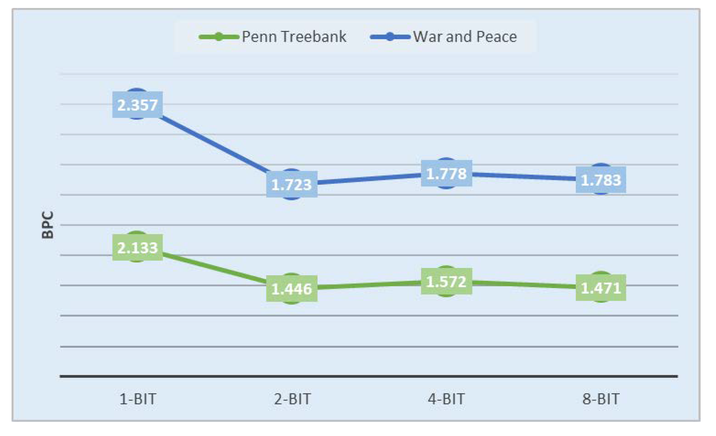
Comparison with Different Bits: To provide a comprehensive view of the BPC value of our quantization method in different quantization precisions, we conducted experiments by directly quantizing the trained full precision weight. The results on War and Peace and Penn Treebank datasets are shown in
Figure 7. Among all the compared multi-bit quantization processes, we can see that our proposed method is still a competitive presence across all varying bits. As the number of bits increases, our method gradually makes more accurate predictions on Character-level language modeling.
4.2.2. Word-Level Language Prediction
In this section, we perform experiments to predict the next word on the Penn Treebank dataset. A one-layer LSTM is verified with d = 300 as in [
33], and d = 650 as in [
34]. We use the same data preparation and training procedures as in [
34]. The optimizer is SGD. The quantization methods are retrained considering the perplexity per word (PPW) metric, which is an index of how “confused” the language model is when predicting the next word. For the 2-bit alternating LSTM, only units = 300 are reported in [
33].
We proposed a benchmark between our results and other works from the literature. To make the benchmark as fair as possible, we consider that other manuscripts working with LSTM-based models are all based on quantization-aware training (QAT). The focus of our comparison is not on the original floating-point accuracy, but rather on the variation in the metric when applying quantization.
Table 4 shows the testing PPW results and size of LSTM parameters with different units. For the 1-bit quantized LSTM, our method and BCN do not achieve comparable performance to the full-precision counterpart. However, in the case of 2-bit quantized LSTM, our method achieves minimum quantization variations of 3.31 and 4.64 compared to the full-precision baseline at the two hidden element counts, respectively, compared to all other methods. Again, in
Table 4, we notice that our method leads to the lowest PPW values, 94.81 and 92.24 lower than all comparison methods shown.
Notice that the comparison is made in terms of bit widths rather than fixed-point arithmetic because other works do not actually consider the hardware application of the obtained quantized models. Our method, instead, is described considering the subsequent hardware implementation of our models on architectures completely based on uniform-symmetric quantization strategy.
To further assess the effects of the other different quantization methods on the single LSTM Layer, we also make a comparison between the results obtained with the proposed quantization method and the results from other works in the literature by the PPW and relative mean squared error (MSE) metric. In LSTM architectures, we have considered hidden units 300.
Table 5 records the PPW and relative MSE of quantized weight matrices with the full-precision. The lowest PPW and relative MSE values are shown in bold. As shown in
Table 5, we can see that our proposed method can achieve the lowest metric across all quantization methods.
Since quantized models usually have comparable or even better performance than the full-precision baseline, it is worth mentioning that our method is lower than the PPW value of the full-precision model at 4-bit precision. This is by no means uncommon in the contrasting method. In other words, the quantization method proposed by the paper not only surpasses the existing classical quantization algorithm under different bit widths on different datasets but also has comparable or even better performance than the full precision baseline.
4.2.3. Image Classification
Deep neural networks (NN) can be categorized into convolution-based NN (ConvNet), fully connected NN (FCNet), and recurrent NN (RNN) [
36]. ConvNet is composed of convolutional and pooling layers and is good at visual feature extraction. FCNet is composed of multiple fully connected layers and is usually used for classification. RNN is composed of fully connected layers with feedback paths and gating operations and performs well in sequential data processing. ConvNet uses Alexnet or Vgg16, etc., to extract spatial features from video frames, and RNN uses LSTM or GRU, etc., to extract sequential features.
In order to verify the advantages of the improved algorithm, this experiment adopted four test models combined with ConvNet + FCNet + RNN for the accuracy test of the classification task. CLDNN [
37], LRCN [
11], AlexNet-LSTM [
38], and Vgg16-LSTM [
11] were selected for comparison. Operators covered by the Vgg16-LSTM classification model architecture are very comprehensive. They include both regular operators such as convolution and emerging complex operators such as LSTM. The sequential images are successively extracted from the image and sequence features, and finally, the classification prediction result of Golf Swing is obtained. All the above contrast test models are trained in the Caffe framework. In this paper, sequential feature-based LSTM quantization algorithm improvements are made to the latter two models. The results are shown in
Table 6, where “
![Applsci 12 12744 i001]()
” indicates that an improved sequential quantization calibration method has been added. It is evaluates the accuracy loss (Acc loss) after quantization.
In general, since the model applied by our method is based on the accuracy of a floating-point model of 32-bit, our technique improves quantization accuracy on average over the fixed 16-bit mode at baseline. In Vgg16-LSTM, RNN takes up a small proportion (9.52%) of total computations, which means acceleration on RNN is not very noticeable compared to ConvNet and FCNet.
4.3. Ablation Experiments
In this section, ablation experiments with the algorithm are conducted on the UCF101 dataset with a sequential quantization calibration design and the activation quantization clipping methods, respectively. UCF101 dataset described by Soomro et al. in [
39] is a video-action recognition classification dataset with 101 categories. A total of 2083 video samples in the first 55 categories were selected as the test dataset on PC and FPGA.
4.3.1. W/ and W/O Sequential Quantization Calibration
To further analyze the effectiveness of the improvements made in sequential quantization calibration design for LSTM, an ablation experiment was performed on the UCF101 dataset.
Different quantization calibration methods are used for AlexNet-LSTM and Vgg-LSTM networks to obtain better accuracy calculation results. The experimental results are shown in
Table 7, where “
![Applsci 12 12744 i001]()
” indicates that an improved quantization calibration method was added, and “
![Applsci 12 12744 i001]()
” without identification indicates that the regular layer’s quantization calibration method (which is mentioned in subsection C of
Section 3) was used. Experimental results show that the accuracy loss of the combined strategy with sequential characteristics adopted for the quantization calibration set is reduced from 1.544% (or 2.707%) to 0.803% (or 1.68%). It confirms that this strategy can improve the accuracy of LSTM quantization deployment.
4.3.2. Comparision between Clipping Methods
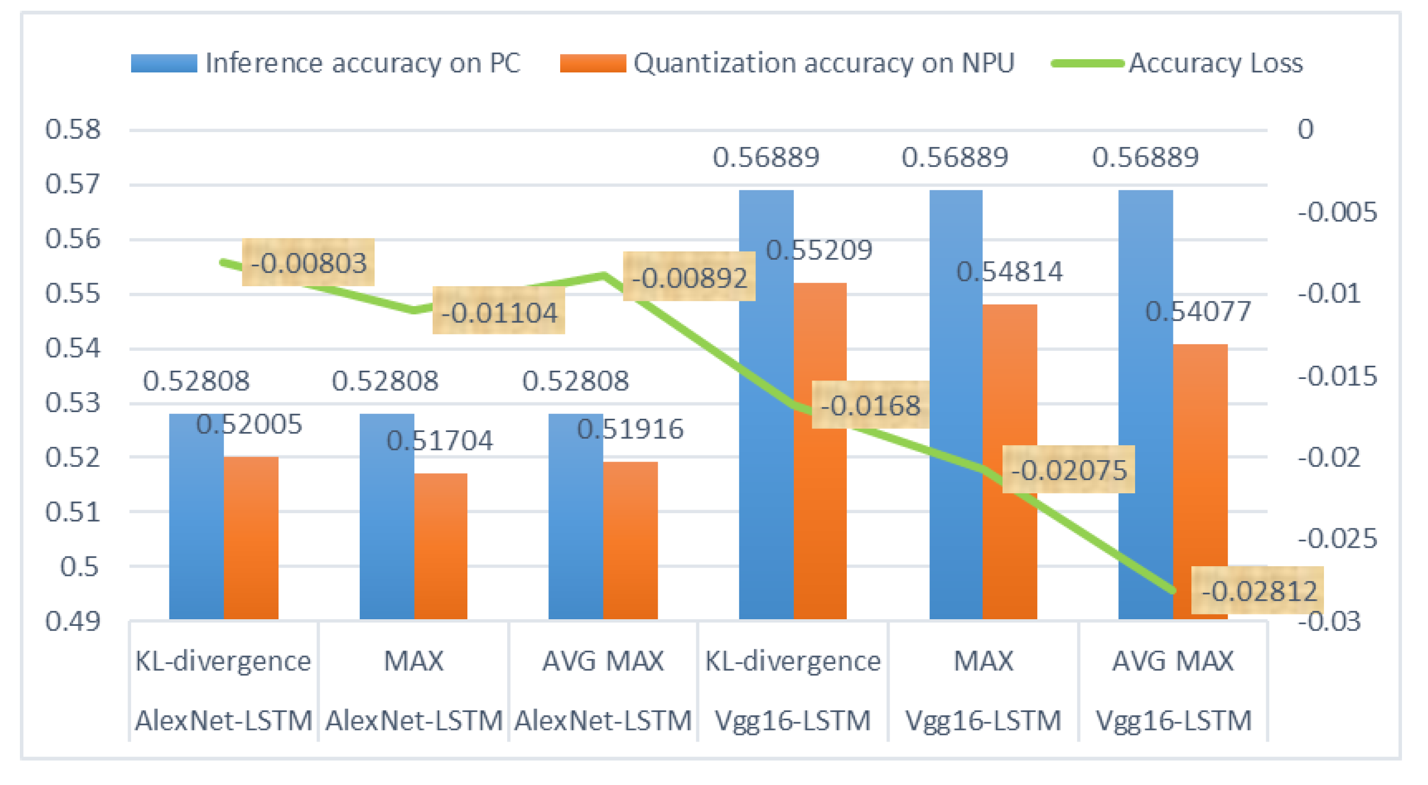
The goal of a quantization algorithm is to generate quantization parameters. The activation threshold for each layer is a quantization parameter that is selected according to the dynamic range of the activation value. After investigation, LSTM layer activation quantization clipping methods include KL-divergence, MIN–MAX, AVG–MAX, Easy Quant, ADMM, etc. Here, the first three were selected for the ablation experiments on the UCF101 dataset.
Table 8 shows the accuracy calculation results of different test models under different activation clipping methods, where “
![Applsci 12 12744 i001]()
” indicates that the corresponding activation clipping method was added. It can be seen from the accuracy loss results that no matter which test model it is based on, and no matter which activation quantization clipping method is used, the quantization loss using the proposed method only differs by 0.803% in the best accuracy and 2.812% in the worst.
In order to show the specific values of the inference accuracy on PC and the calculation accuracy on NPU in more detail, we have plotted the following comparative experiment based on different test models. The quantization accuracy experiments in
Figure 8 show that, compared with the inference accuracy on PC, the model deployed on the NPU using the proposed method reflects high accuracy loss and the practical value of the proposed quantization method.
Therefore, these two ablation experiments show that the operator disassembly operation of the LSTM layer can solve the problem that the existing NPU cannot directly compute the LSTM layer.
4.4. Performance Analysis
It is very important to measure the deployment performance of the model on different platforms, and it has a strong reference for improving the quantization scheme and FPGA hardware design. Since the speed of simulating NPU calculations on the PC side is slower, we deployed the proposed method to a real NPU, embedding the core calculations of the model on the neural network accelerator. Quantization and classification prediction are carried out on the neural network accelerator.
The experiments on the PC were carried out on Windows 10. The CPU is Intel(R) Core(TM) i7-8700 K, 3.70 GHz, the GPU is NVIDIA GeForce GTX1070, and the deep learning framework is Torch 1.4.1 and Caffe. The experiment on NPU uses the TIANJI NPU3.0 neural network accelerator proposed by Xi’an Microelectronics Technology Institute [
40]. This accelerator is implemented based on Xilinx ZCU102 FPGA, with self-controllable IP and the application development tool chain. It supports multi-model online switching and pipeline parallel acceleration [
41]. It supports real-time detection and positioning applications of satellites, spacecrafts, and other targets and can meet the needs of visual ranging and intelligent obstacle avoidance applications.
We test the running speed of LRCN models of different backbone networks on the CPU, GPU, and NPU, respectively. At the same time, the running speed of the backbone network itself on the NPU was also tested. Moreover, the specific speed of the LSTM layer was obtained by the difference between the execution speed of the AlexNet-LSTM or Vgg16-LSTM networks and the backbone network (AlexNet or Vgg16) on the NPU. Note that the execution speed here is the average model deployment time over a single time step. The details are shown in
Table 9.
Experiments show that the execution speed of the AlexNet-LSTM model on the neural network accelerator is 1.6 times faster than on the CPU and 1.3 times faster than on the GPU. The Vgg16-LSTM model is executed fastest on the GPU due to the small filter size and large model depth. The execution time is 39.7 ms. The execution time on the neural network accelerator is still 1.87 times faster than on the CPU. Moreover, from the data point of view, a single time step of the LSTM with the hidden state output feature dimension of 256 on the NPU is about 1 ms at 20 W power consumption.


 ” indicates that an improved sequential quantization calibration method has been added. It is evaluates the accuracy loss (Acc loss) after quantization.


